Effect of Square Cap on Pile-Group Wave Force: Parametric Analysis and Case Study

Abstract

The square cap is a typical semi-submersible component of sea-crossing bridges, which connects piers and pile-group foundations. As the cap size is large, it usually has a non-negligible influence on the wave motion around the pile-group foundation, so it is not considered in the relevant specification. However, neglecting this influence may have adverse effects on the structure. In this paper, the wave forces on capped pile groups are simulated by a numerical wave flume. Firstly, the numerical flume used in this paper is validated by an experiment in the previous literature. Then, capped pile groups with different arrangements and different water levels are modeled to study the interference effect of the square cap on the wave force, and the variation law of the interference effect coefficient $K_{cp}$ of the cap is given. Next, we introduce $K_{cp}$ into the theoretical formula of wave forces on pile groups and obtain a modified formula that considers the cap effect. To verify the feasibility of the modified formula in practical engineering, we use the formula to calculate the wave forces acting on capped pile groups of a sea-crossing bridge. The results of the modified theoretical formula are compared with that of the numerical water flume and recommended values in the specification. It is found that the theoretical values are relatively close to the numerical results, while the specification values tend to be conservative. The modified theoretical formula proposed in this paper and the obtained parameter distribution law can provide a reference for engineering design.

1. Introduction

In recent years, numerous sea-crossing bridges have been constructed worldwide. However, during the life cycle of these bridges, the harsh marine environment [1], including hurricanes and ocean currents, can severely impact their service life and even cause instability or structural damage [2], leading to potentially disastrous safety incidents. Most highway bridge destruction can be attributed to bridge collapse due to wave load impacts [3]. Consequently, the design of wave load on the foundation structure of a sea-crossing bridge has emerged as a key component of the entire bridge design. Wave force is influenced by environmental factors such as water level and flow velocity as well as factors such as pile group arrangement, pile diameter, and cap size [4].

In the last century, scholars began conducting extensive research on calculating wave force on the pile-group foundations of sea-crossing bridges [5,6]. The Morison formula [7], derived from potential flow theory, is one of the most famous semi-theoretical formulas for calculating horizontal wave force on a small-scale vertical cylinder. However, the hydrodynamic coefficients for the inertial force and drag force in the formula are affected by various factors such as the Reynolds number and KC number, and their values must be determined precisely through experiments [8], which has paved the way for the development of related experimental research. Thereafter, Sarpkaya and Justesen [9,10] obtained the force coefficient through numerous wave flume experiments. Based on their work, Boccotti [11] conducted further experiments to study how the coefficients vary with the KC number and Re number. It is worth noting that the Morison formula is no longer applicable to large-scale structures such as pile groups and foundations, as waves reflect and diffract between such structures. MacCamy [12] first proposed a diffraction theory based on the assumption of small-amplitude linear waves. Neelamani [13] further verified the accuracy of the diffraction theory by carrying out a water flume test. Garrison [14] has also regulated the Morison equation and diffraction theory’s applicable range. Terro [15] modified the linear form of the Morison equation based on the numerical water flume, making it more accurate for nonlinear wave force estimation.

Although significant improvements have been made to theoretical methods, their application is still limited. For such cases, the physical water flume experiment is an appealing solution. Liu [16] used a three-dimensional flume to determine the reduction coefficient of the wave force on a pile group by analyzing the force of four different types of inclined piles on the East Sea Bridge. Qu [17] proposed a method to assess the total wave force using the effective diameter, which was determined through wave flume experiments. Based on this, an empirical formula was developed to calculate the wave force of various pile-supported structures in regular and irregular waves. Zhang [18,19] conducted wave flume experiments to study the wave force on pile groups with different arrangements under varying wave conditions. Moreover, Bonakdar [20] used an artificial intelligence data analysis method to derive a new calculation formula for pile-group wave force based on wave flume experiments. However, the physical experiment is costly and has low universality, which brings many inconveniences to researchers when a large number of experiments are needed.

With the progress of computer technology, numerical flumes have developed rapidly, greatly reducing the time, economic costs, and labor costs required for experiments. Many scholars have also verified the accuracy of the numerical flume through comparisons with physical experiments [21]. Dong [22] studied the generation and propagation of the wave in a numerical viscous wave flume and accurately generated several incident waves. Huang [23] created a two-dimensional wave–current interaction model and then proposed an empirical equation for the wave–current force acting on a box girder bridge. Deng [24] investigated the influences of wave height, wave length, cap dimension, and submerged depth on the cap effects through a numerical water flume. All these lay the foundation for solving the wave force of the pile group by numerical flume. However, research on the interaction between the cap and the pile group is limited, and the influence of pile arrangements and water levels on wave forces is rarely considered.

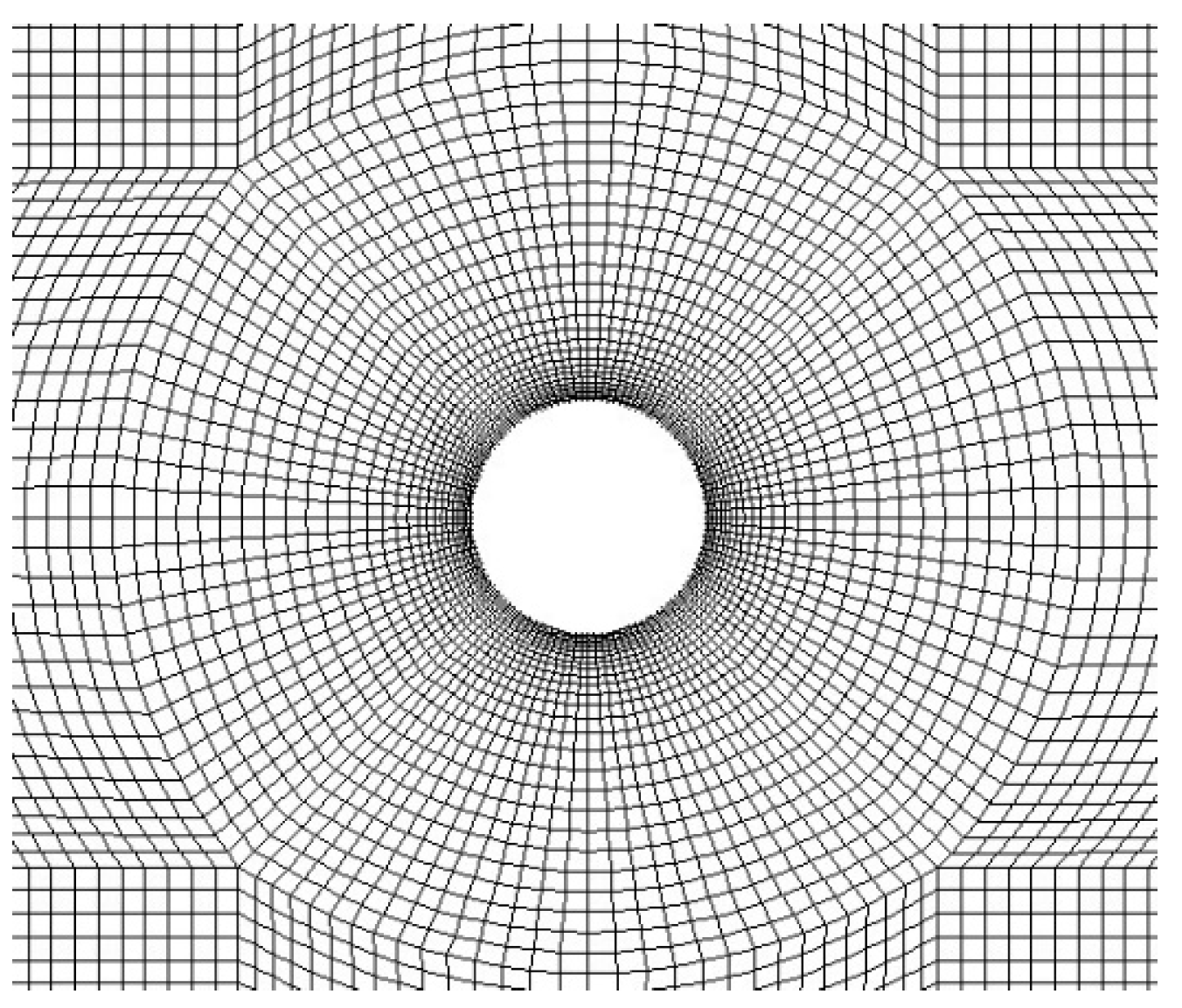
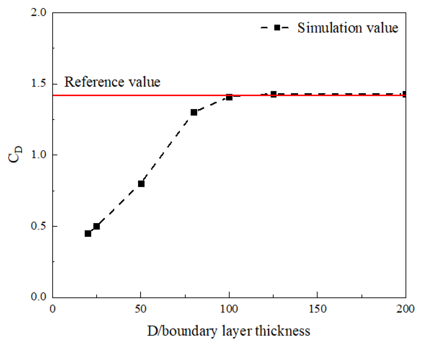
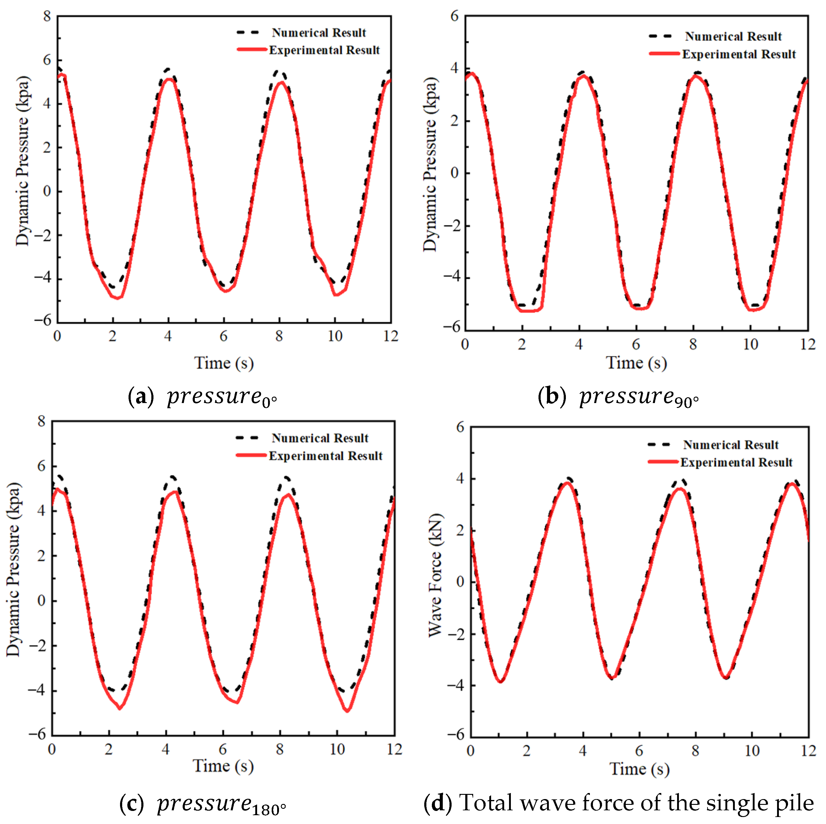
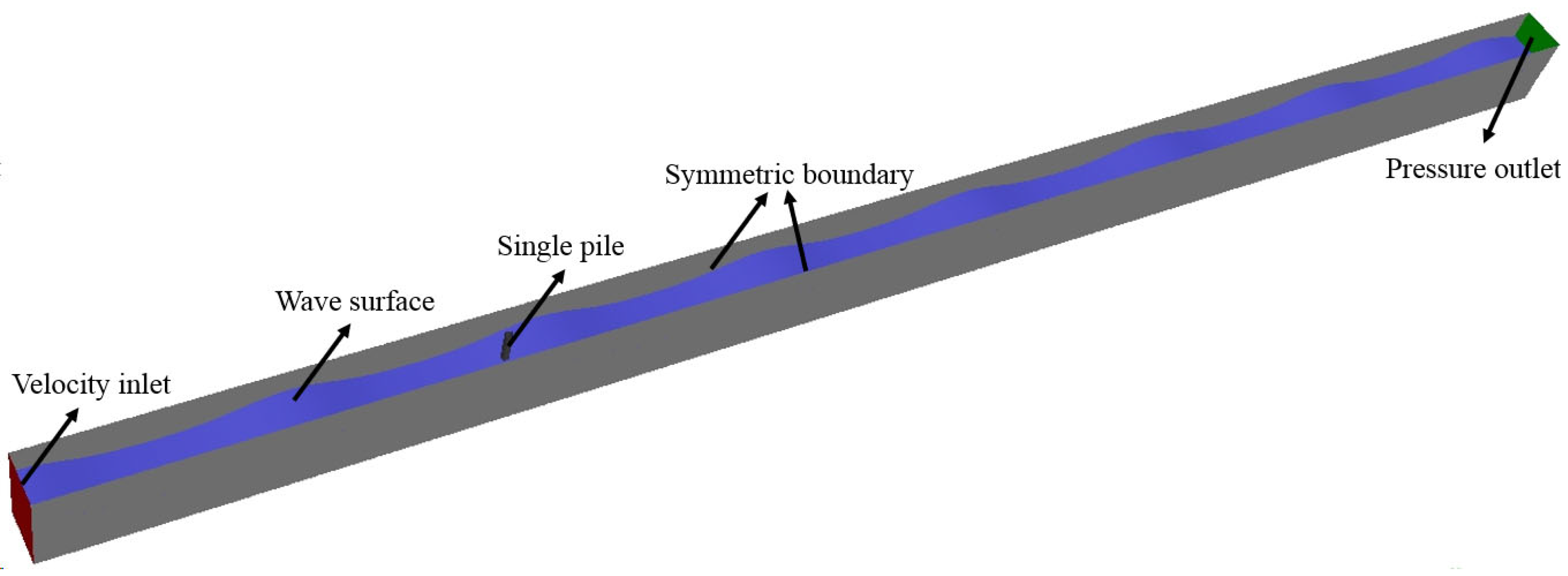
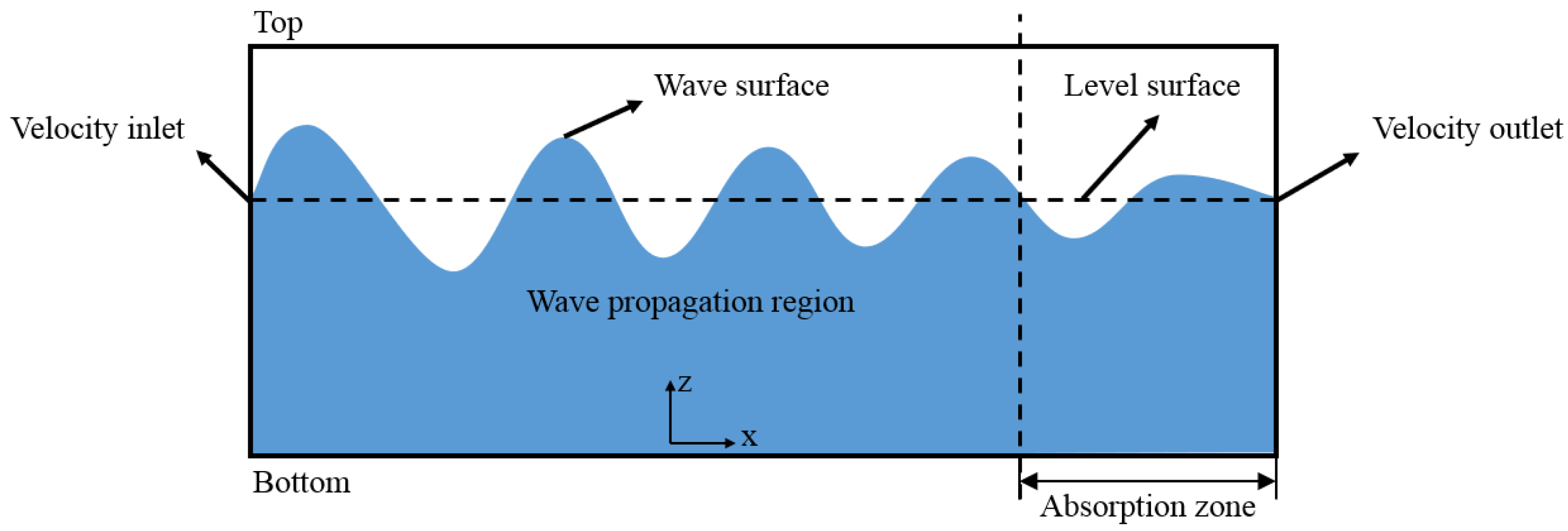
This paper aims to reveal the influence of the cap on wave forces acting on pile groups through a three-dimensional numerical water flume. The remainder of this paper is organized as follows. Section 2 briefly introduces the numerical methods used and the validation of the numerical flume, including wave generation and elimination, the grid size, and the boundary conditions. The numerical flume has been validated with the test results of the physical flume in the relevant literature. In Section 3, the influence of the cap on the wave forces acting on the pile group with different arrangements and water levels is studied. In Section 4, we establish a modified theoretical formula for calculating wave forces considering the cap effect. In Section 5, an engineering project is simulated to verify the feasibility of the modified theoretical formula proposed in this paper. Conclusions are drawn in Section 6.

2. Numerical Methods and Validation

2.1. Numerical Methods

2.1.1. Governing Equations

The governing equations for our fluid simulation include the continuity equation and momentum equation [25]:

$$\frac{\partial \rho }{\partial t}+\nabla \cdot \left(\rho \mathit{u}\right)=0$$

(1)

$$\frac{\partial \left(\rho u_i\right)}{\partial t}+\nabla \left(\rho u_i\mathit{u}\right)=\nabla \left(\mu \mathrm{g}\mathrm{r}\mathrm{a}\mathrm{d}{u}_i\right)-\frac{\partial p}{\partial x_i}+S_{u_i}$$

(2)

in which $\rho$ is the density of fluid; $\mathit{u}$ is the velocity vector and $u_i$ are fluctuating velocity components; and $p$ is pressure. $\mu$ is viscosity coefficient; grad = $\frac{\partial }{\partial x}+\frac{\partial }{\partial y}+\frac{\partial }{\partial z}$ is the gradient; and $S_{u_i}$ is the generalized source term of the momentum conservation equation.

The Reynolds-averaged Navier–Stokes (RANS) equations are the most widely used method for turbulence. This model establishes assumptions about the Reynolds stress through turbulence theory and observations, generating a series of empirical or semi-empirical constitutive relations that enable the closure of the motion equation of turbulence. Temperature changes are ignored in this analysis, conducted at room temperature. The conservations of the mass and momentum in the RANS equations are as follows:

$$\frac{\partial \rho }{\partial t}+\frac{\partial }{\partial x_i}\left(\rho u_i\right)=0$$

(3)

$$\frac{\partial \left(\rho u_i\right)}{\partial t}+\frac{\partial }{\partial x_j}\left(\rho u_i{u}_j\right)=-\frac{\partial p}{\partial x_i}+\rho g_i+\frac{\partial }{\partial x_j}[\mu \left(\frac{\partial u_i}{\partial x_j}+\frac{\partial u_j}{\partial x_i}\right)-\rho \overline{u_i^{\prime }{u}_j^{\prime }}]$$

(4)

in which $i$ and $j$ represent the directions of the coordinates $(x;y;z)$; $g_i$ is the acceleration; $\rho \overline{u_i^{\prime }{u}_j^{\prime }}$ is the Reynolds stress which represents the effects of the turbulent flow on the mean flow field. Recently, the RANS method has been applied to wave simulation and has achieved good results [26]. Finnegan [27] compared turbulence flow models and found that there was no difference in the height of waves generated between the models, so the turbulence model is not a factor in the generation of waves using a wave-maker. In addition, in this article, we chose the k-ω model [28,29].

2.1.2. Volume-of-Fluid Method

Establishing a numerical flume also requires an accurate description of the free surface, that is, the interface between the air and water phases [30]. This paper uses the volume-of-fluid (VOF) method. The VOF method introduces a fluid volume fraction, ${\alpha }_n$, defined as the ratio of the volume of the n-th phase fluid to the total volume of the grid in a certain grid. The numerical wave flume established in this paper only involves two phases, air and water, as schematically shown in Figure 1. The free surface can be described as follows:

$${\alpha }_2=\left\{\begin{array}{c}0, \mathrm{a}\mathrm{i}\mathrm{r}\\ 0<{\alpha }_2<1, \mathrm{f}\mathrm{r}\mathrm{e}\mathrm{e} \mathrm{s}\mathrm{u}\mathrm{r}\mathrm{f}\mathrm{a}\mathrm{c}\mathrm{e}\\ 1, \mathrm{w}\mathrm{a}\mathrm{t}\mathrm{e}\mathrm{r}\end{array}\right.$$

(5)

Free surfaces are extracted from ${\alpha }_2=0.5$. The following equations must be satisfied by the volume fraction ${\alpha }_n$:

$$\left\{\begin{array}{c}\frac{\partial {\alpha }_n}{\partial t}+\frac{\partial \left(u{\alpha }_n\right)}{\partial x}+\frac{\partial \left(v{\alpha }_n\right)}{\partial y}=0\\ {\displaystyle \sum _{n=1}^2}{\alpha }_n=1\end{array}n=\mathrm{1,2}\right.$$

(6)

2.2. Validation of the Numerical Wave Flume

The thickness of the boundary layer grid on the surface of the structure will have an impact on the results. In this section, we first verify the sensitivity of the numerical grid. This section selects a two-dimensional cylindrical flow for research, and liquid water is used as the fluid. The boundary layer grid thickness and the overall grid are simulated and analyzed for size impact, in which $D/200$, $D/125$, $D/100$, $D/80$, $D/50$, $D/25$, and $D/20$ are selected for the boundary layer grid, and $D/10$ is selected for the overall grid, in which D is the diameter of the cylinder. The grid of the $D/100$ boundary layer is shown in Figure 2.

Calculate the drag coefficient of different simulation results according to the following formula:

$$F_D=\frac{1}{2}{C}_D\rho U^{2}D$$

(7)

in which $F_D$ is the cylinder resistance. The $C_D$ results of different cases of boundary layer grid thickness are shown in Figure 3. It can be seen from the results that when the boundary layer grid thickness is less than or equal to $D/100$, the error between the simulated value and the value in reference [31] is already small, so the boundary layer thickness of about $D/100$ can be used in the simulation to obtain more accurate results.

A comparison between the numerical wave flume and the corresponding physical experiment [32] is made here to validate the numerical wave flume. The experimental setup involves a wave flume with a depth of 7 m, a width of 5 m, and an effective length of 309 m. For the experiment, a cylinder with a diameter of 0.7 m is positioned 110 m away from the wave-generating plate, with wave gauges, strain gauges, current meters, and pressure cells arranged on the cylinder. The wave parameters are presented in

Table 1. Wave parameters for validation.

Wave Type	$\mathbf{Depth} \mathit{d}/\mathbf{m}$	$\mathbf{Period} \mathit{T}/\mathbf{s}$	$\mathbf{Wave} \mathbf{Height} \mathit{H}/\mathbf{m}$	$\mathbf{Wave} \mathbf{Number}\mathit{k}/{\mathbf{m}}^{-1}$
Regular wave	4.76	4	1.2	0.2735

. The test device is shown in Figure 4. We used ANSYS Fluent 19.0 to establish the numerical water flume.

As depicted in Figure 5, the numerical wave flume utilized in this study possesses a length of 160 m, a width of 5 m, and a height of 8 m. The distance between the structure and the inlet is 40 m. The inlet is designated as the velocity inlet, while the outlet and top are the pressure outlets. Symmetrical boundaries are assigned to the flume’s two sides, while non-slip boundaries are used for the column and the bottom. The overall grid size is set as $D/10,$ whereas the grid size of the cylinder and the bottom boundary layer is set as $D/100$, as illustrated in Figure 6 [33]. Three pressure measuring points are arranged in the same positions as those of the experiment, ${\mathrm{p}\mathrm{r}\mathrm{e}\mathrm{s}\mathrm{s}\mathrm{u}\mathrm{r}\mathrm{e}}_{0^{°}}$, ${\mathrm{p}\mathrm{r}\mathrm{e}\mathrm{s}\mathrm{s}\mathrm{u}\mathrm{r}\mathrm{e}}_{{90}^{°}}$, and ${\mathrm{p}\mathrm{r}\mathrm{e}\mathrm{s}\mathrm{s}\mathrm{u}\mathrm{r}\mathrm{e}}_{{180}^{°}}$. In addition, the time interval is 0.01 s.

Furthermore, the paper utilizes an absorption zone to eliminate the wave reflection on the outlet boundary [34]. Specifically, an artificial damping term is added to the momentum equation [35]. A schematic diagram of the numerical water flume is shown in Figure 7.

For wave generation, the velocity distribution of the water points and wave surface at the entrance are set according to the Fenton formula [36] to generate regular waves. A comparison between the experiment results and the numerical results of the three pressure measuring points, ${pressure}_{0^{°}}$, ${pressure}_{{90}^{°}}$, and ${pressure}_{{180}^{°}}$, is presented in Figure 8a–c. Dynamic pressure refers to the total pressure minus the static pressure. A comparison of the total wave force on the single pile is also displayed in Figure 8d.

It can be seen that the results obtained by the numerical water flume are uniform sine waves in the stable stage, while the actual test is influenced by the equipment and instruments, and the results are not completely consistent within each cycle. However, as depicted in these graphs, the error between the numerical and experimental results is negligible. The results of the threedimensional numerical wave flume established in this paper are consistent with the corresponding experiment results. Hence, utilizing the numerical wave flume to investigate structures’ wave forces is reliable.

3. The Influence of Different Pile Arrangements and Water Levels

A bridge’s pile-group foundation structure typically comprises two components: the cap and the pile group. A large cap can cause significant disruption to the surrounding wave field, thereby affecting the wave force on the pile group. In this section, the numerical wave flume is applied to study the effect of caps on pile-group wave forces across various pile arrangements and water levels.

3.1. Different Arrangements

Three different capped pile groups are simulated: two piles arranged in the vertical wave direction, two piles parallel to the wave direction, and four piles arranged in two rows and two columns. The parameters of the three cases are shown in

Table 2. Simulation cases of capped pile group.

Case	Arrangement	Pile Diameter $/\mathbf{m}$	$\mathbf{Center} \mathbf{Distance} \mathbf{of} \mathbf{Pile} \mathit{l}/\mathbf{m}$	Height of Cap $\mathit{h}/\mathbf{m}$	Width of Cap $\mathit{b}/\mathbf{m}$	Length of Cap $\mathit{L}/\mathbf{m}$
1		1	2	1	4	2
2		1	3	1	5	2
3		1	2	1	2	4
4		1	3	1	2	5
5		1	4	1	2	6
6		1	2	1	4	4
7		1	3	1	5	5

. Three different distances between the pile centers are investigated. Fifth-order Stokes waves with a wave height of 0.73 m and a wavelength of 15 m are utilized. The water level is set at the midpoint of the cap height, and the water-level coefficient $C_w$ is 0.5. The length of the numerical wave flume is 60 m, and the water depth is 7 m. The pile-group foundation structure is set at a distance of 20 m from the wave-making inlet. Only the meshing of case 6 is shown in Figure 9a. The wave surface velocity contour of the numerical flume at a certain time under three arrangement cases are shown in Figure 9b–d (cases 1, 3, and 6), respectively.

3.1.1. Two Piles Arranged in Vertical Wave Direction

The initial two simulation cases feature two piles arranged in the vertical wave direction, albeit with different distances between their centers. We can obtain the wave-force time histories for each pile, which we can then compare to those obtained without a cap for the same cases. The comparisons are displayed in Figure 10. As shown in Figure 8, each capped pile experiences a decreased wave force compared to the uncapped scenario. Moreover, the cap structure has a more pronounced reduction effect on the peak value of the wave force than the valley value.

The interference coefficient $K_{cp}$ of the cap on the pile can be defined as follows:

$$K_{cp}=\frac{F_{with cap}}{F_{without cap}}$$

(8)

where $F_{with cap}$ is the extreme value of wave force on capped piles, and $F_{without cap}$ is that on piles without a cap. The average values of the peak and valley values of the wave forces of the two piles in the above cases are obtained as shown in

Table 3. Cap-interference coefficient of multiple capped piles arranged in vertical wave direction.

Pile Number	Center Distance of Pile	$\mathbf{Wave} \mathbf{Force} \mathbf{without} \mathbf{Cap}/\mathbf{k}\mathbf{N}$		$\mathbf{Wave} \mathbf{Force} \mathbf{with} \mathbf{Cap}/\mathbf{k}\mathbf{N}$		$\mathbf{Cap}-\mathbf{Interference} \mathbf{Coefficient} {\mathit{K}}_{\mathit{c}\mathit{p}}$
		Peak Value	Valley Value	Peak Value	Valley Value	Peak Value	Valley Value
1	2$D$	6.42	6.32	5.22	5.65	0.81	0.89
	3$D$	6.12	6.05	4.95	5.62	0.81	0.93
2	2$D$	6.42	6.32	5.23	5.65	0.81	0.90
	3$D$	6.12	6.05	4.96	5.62	0.81	0.93

, as well as $K_{cp}$.

We can infer from Table 3 that the position of the pile, the distance between pile centers, and the width of the pile have little effect on the cap-interference coefficient of the peak wave force when arranged in the vertical wave direction. It is worth noting that the interference coefficient of the peak value is lower than that of the valley value as the cap has more noticeable interference effects on the peak wave force.

3.1.2. Two Piles Arranged in Parallel Wave Direction

Cases 3 to 5 are two piles arranged in parallel wave directions with different pile-center distances. Compared with the corresponding non-cap case results, the cap-interference coefficient is calculated as shown in

Table 4. Cap-interference coefficient of multiple capped piles arranged in parallel wave direction.

Pile Number	Center Distance of Pile	$\mathbf{Wave} \mathbf{Force} \mathbf{without} \mathbf{Cap}/\mathbf{k}\mathbf{N}$		$\mathbf{Wave} \mathbf{Force} \mathbf{with} \mathbf{Cap}/\mathbf{k}\mathbf{N}$		$\mathbf{Cap}-\mathbf{Interference} \mathbf{Coefficient} {\mathit{K}}_{\mathit{c}\mathit{p}}$
		Peak Value	Valley Value	Peak Value	Valley Value	Peak Value	Valley Value
1	2$D$	4.98	5.33	3.80	4.27	0.76	0.80
	3$D$	5.25	5.44	3.82	4.17	0.73	0.77
	4$D$	5.83	6.01	4.04	4.43	0.69	0.74
2	2$D$	5.23	5.32	4.13	4.31	0.79	0.81
	3$D$	5.40	5.49	4.17	4.39	0.77	0.80
	4$D$	5.78	5.95	4.39	4.61	0.76	0.78

.

As shown in Table 4, the interference coefficient of the cap for front pile 1 decreases as the distance between pile centers increases. Similarly, there is a modest decrease in the interference coefficient of the cap for rear pile 2 as the distance between pile centers expands.

It can be observed that different pile-center distances have distinct impacts in the case of two piles arranged in the parallel wave direction. For pile 1, the center distance will change the length of its rear cap, without affecting the length of its front cap; for pile 2, the center distance will change the length of its front cap without affecting the length of its rear cap. For convenience, we define the cap length on the front side of the pile, denoted by $d_f$, as the distance from the pile center to the front side of the cap and, similarly, the cap length on the backside of the pile, denoted by $d_b$, as the distance from the pile center to the backside of the cap.

(1) The influence of $d_b$ on the cap-interference coefficient.

Based on our analysis of the cap-interference coefficient of two piles arranged in the vertical wave direction in the previous section, we observed that the lateral position and width of the cap have minimal effects on the cap-interference coefficient of the two piles. Rather, the length of the cap on either side of the pile significantly affects the cap-interference coefficient. By combining the results in this section, we can depict the changes in the cap-interference coefficient of pile 1 as a function of the length of the cap at the back of the pile, as illustrated in Figure 11.

As shown in the figure, when the length of the cap on the front side of the pile remains constant, the interference coefficient decreases as the length of the cap on the backside of the pile increases. In other words, the greater the length of the cap on the backside, the stronger the interference effect. Moreover, we observe that the interference coefficient of the wave-force valley value is slightly larger than that of the peak value.

(2) The influence of $d_f$ on the cap-interference coefficient.

Likewise, we present the changes in the cap-interference coefficient of pile 2 in Figure 12. It is apparent that when the length of the cap behind the pile remains constant, the cap-interference coefficient increases as the length of the cap in front of the pile extends. Moreover, we notice that the interference coefficient of the wave-force valley value is slightly greater than that of the peak value.

3.1.3. Four Piles Arranged in Two Rows and Two Columns

Cases 6 and 7 are four piles arranged in two rows and two columns with different pile-center distances. Compared with the corresponding non-cap case results, the cap-interference coefficient is calculated as shown in

Table 5. Cap-interference coefficient of multiple capped piles arranged in two rows and two columns.

Pile Number	Center Distance of Pile	$\mathbf{Wave} \mathbf{Force} \mathbf{without} \mathbf{Cap}/\mathbf{k}\mathbf{N}$		$\mathbf{Wave} \mathbf{Force} \mathbf{with} \mathbf{Cap}/\mathbf{k}\mathbf{N}$		$\mathbf{Cap}-\mathbf{Interference} \mathbf{Coefficient} {\mathit{K}}_{\mathit{c}\mathit{p}}$
		Peak Value	Valley Value	Peak Value	Valley Value	Peak Value	Valley Value
1	2$D$	5.29	5.53	3.96	4.44	0.75	0.80
	3$D$	5.53	5.51	4.04	4.22	0.73	0.77
2	2$D$	5.25	5.52	3.93	4.44	0.75	0.80
	3$D$	5.51	5.45	4.04	4.22	0.73	0.77
3	2$D$	5.67	5.71	4.40	4.52	0.78	0.79
	3$D$	5.66	5.64	4.27	4.42	0.75	0.78
4	2$D$	5.75	5.64	4.47	4.48	0.78	0.79
	3$D$	5.66	5.64	4.27	4.42	0.75	0.78

.

It is apparent from Table 5 that the interference coefficients of the adjacent piles (pile 1 and pile 2, as well as pile 3 and pile 4) in the vertical wave direction are equal, implying that the location of different vertical wave directions does not affect the cap-interference coefficient. On the other hand, the arrangement positions of the piles in the parallel wave direction and the pile-center distances influence the cap-interference coefficient. As presented in

Table 6. Comparison of interference coefficients between two piles arranged in parallel wave direction and four piles arranged in two rows and two columns.

Pile Position	Center Distance of Pile	Peak Value			Valley Value
		Two Piles	Four Piles	Error	Two Piles	Four Piles	Error
Front	2D	0.76	0.75	−1.32%	0.80	0.80	−0.35%
	3D	0.73	0.73	−0.45%	0.77	0.77	−0.04%
Rear	2D	0.79	0.78	−1.27%	0.81	0.79	−2.47%
	3D	0.77	0.76	−1.30%	0.80	0.78	−2.50%

, we compare the cap-interference coefficients of pile 1 and pile 3 arranged in the parallel wave direction of this section with those of the two piles in cases 4 and 5. Table 6 indicates that the two arrangements’ interference effect coefficients of the corresponding pile positions are the same. Thus, for multi-row capped pile groups, we can calculate the cap-interference coefficient of each row of piles in the parallel wave direction based on the corresponding single row of piles.

3.2. Different Water Levels

When the cap’s submerged depth varies, so does the interference with the pile group. In this section, the two capped piles arranged in the vertical wave direction with three different water-level coefficients are simulated. The simulation cases are shown in

Table 7. Simulation cases of different water levels.

Case	$\mathbf{Water}-\mathbf{Level} \mathbf{Coefficient}{\mathit{C}}_{\mathit{W}}$	$\mathbf{Pile} \mathbf{Diameter} \mathit{D}/\mathbf{m}$	$\mathbf{Center} \mathbf{Distance} \mathbf{of} \mathbf{Pile} \mathit{l}$	$\mathbf{Height} \mathbf{of} \mathbf{Cap}\mathit{h}/\mathbf{m}$	$\mathbf{Width} \mathbf{of} \mathbf{Cap}\mathit{b}/\mathbf{m}$	$\mathbf{Length} \mathbf{of} \mathbf{Cap}\mathit{b}/\mathbf{m}$
1	0	1	2$D$	1	4	2
2	0.5	1	2$D$	1	4	2
3	1.0	1	2$D$	1	4	2

. The wave distribution contour along the wave-direction section of pile 1 in the simulation is shown in Figure 13.

We obtain the wave-force time history of the two piles in three cases, which is then compared with the results of the corresponding non-cap situation, as illustrated in Figure 14. It is observable from the figure that when the cap is not submerged, the extreme value of the wave force on the pile is similar to the corresponding result of the non-cap case. As the cap’s submerged depth increases, the cap’s interference on the pile’s wave force also elevates.

Table 8. The cap-interference coefficient $K_{cp}$ of different water levels.

$\mathbf{Water}-\mathbf{Level} \mathbf{Coefficient}{\mathit{C}}_{\mathit{W}}$	Pile 1		Pile 2
	Peak Value	Valley Value	Peak Value	Valley Value
0	1.00	0.96	1.00	0.96
0.5	0.81	0.89	0.81	0.89
1.0	0.63	0.63	0.63	0.63

displays the result of the cap-interference coefficient of the two piles in various water-level scenarios. It can be observed that the cap-interference coefficients of pile 1 and pile 2 are identical. Moreover, the interference effect of the cap strengthens with an increase in the water-level coefficient, leading to a decrease in the cap-interference coefficient.

4. Modified Theoretical Formula for Calculating Wave Forces Considering Cap Effect

We introduce $K_{cp}$ into the theoretical formula of wave forces on pile groups [37], which can be expressed as follows:

$$F_p\left(t\right)=\sum K_{cp}{K}_S{K}_I·F_i\left(t\right)$$

(9)

where $F_p\left(t\right)$ is the wave-force time history of the whole pile group, and $F_i\left(t\right)$ is the wave-force time history of every single pile calculated by the Morison formula.$K_{cp}$ is the cap-interference coefficient. $K_S$ is the shelter effect coefficient. $K_I$ is the interference effect coefficient.

The shelter effect coefficient $K_S$ can be calculated as follows:

$$K_S=\frac{F_{c1}}{F_s}$$

(10)

where $F_{c1}$ is the wave force of a single pile in the pile group arranged in the parallel wave direction, and $F_s$ is the wave force on a single pile.

Similarly, the interference effect coefficient $K_I$ can be calculated as follows:

$$K_I=\frac{F_{c2}}{F_s}$$

(11)

where $F_{c2}$ is the wave force of a single pile in the pile group arranged in the vertical wave direction, and $F_s$ is the wave force of a single pile.

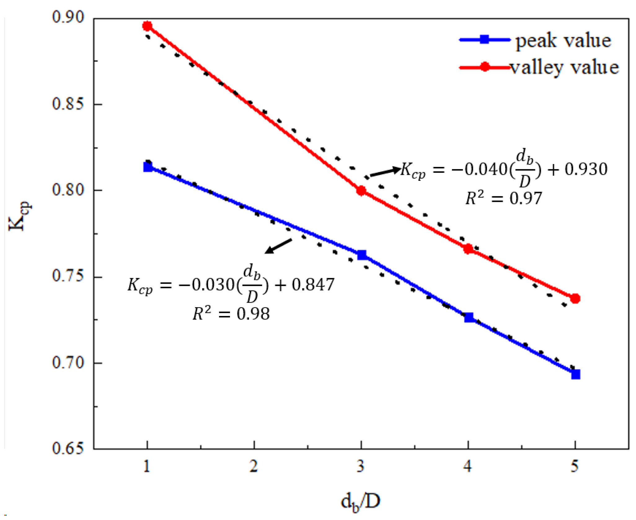
The value of $K_{cp}$ could not be found in the specifications or standards currently. In this paper, it can be assumed that $K_{cp}$ between each row of piles in the parallel wave direction is the same according to Section 3. For each column of piles in a perpendicular wave direction, $K_{cp}$ can be selected according to the front and rear positions of the piles. 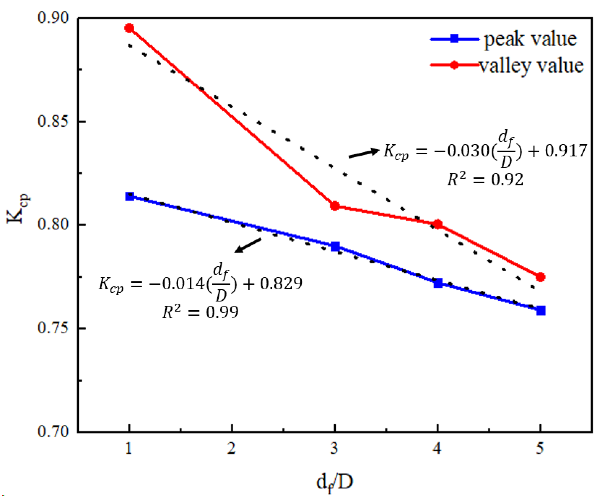The cap-interference coefficient of the front row pile can be linearly interpolated according to the length $d_b$ of the back side pile cap according to Figure 8. Similarly, the cap-interference coefficient of the back row pile can be linearly interpolated according to the length $d_f$ of the front side pile cap according to Figure 9. Considering that the pile cap has a stronger interference effect on the peak wave force and a weaker interference effect on the valley value, the interference coefficient of the valley value can be taken safely. A more unfavorable value can be obtained for the pile groups with more than two columns.

5. Engineering Project Application of a Sea-Crossing Bridge

To verify the accuracy of the modified theoretical formula and the feasibility of the numerical water flume, we selected a sea-cross bridge as the project background in this section and compared the theoretical calculation formula with numerical results.

5.1. Project Description

5.1.1. Overview of Bridge and Foundation Structure

The engineering background selected in this section is the pile-group foundation structure of Xinghua Bay Bridge. The Xinghua Bay Bridge Section includes two main channels, Mulanxi and Diluxi. The schematic diagram of the bridge site is shown in Figure 15.

The main bridge is a four-span variable cross-section steel structure, and the approach bridge is a four-span continuous beam bridge. The pile-group foundation structure of the main bridge has two arrangement forms. The foundation of the three piers of the two main spans is an integrated pile-group structure with two rows and seven columns. The side span foundation includes two split pile groups arranged in two rows and two columns. The caps of the above foundations are square caps. The schematic diagram is shown in Figure 16a,b. The approach section close to the side span also adopts two split pile-group structures with two rows and two rows, and the rest adopt two single-row pile foundation structures, as shown in Figure 16c,d.

The dimensions of the above four pile-group foundations are shown in

Table 9. The dimensions of the four pile-group foundations (m).

	$\mathit{D}$	b × l	$\mathit{h}$	${\mathit{l}}_{\mathit{l}}$	${\mathit{l}}_{\mathit{t}}$	${\mathit{d}}_{\mathit{l}}$	${\mathit{d}}_{\mathit{t}}$	${\mathit{l}}_{\mathit{c}}$
Main span	2.5	34.5 × 11.4	4.5	6	5	2.7	2.25	integration
Side span	2.2	10 × 8.8	3.5	5.2	6.2	1.8	1.9	8
Approach bridge close to the side span	1.8	9 × 6.9	2.5	3.6	5.5	1.65	1.75	9
Others	2.5	13 × 4	2.5	-	9	2	2	5

.

5.1.2. Statistics of Wave Parameters at the Bridge Site

The wave characteristics in this area are mainly mixed waves dominated by the monsoon. The wave height distribution with a recurrence period of 100 years is shown in Figure 17.

The wave parameters of the above four pile-group foundations are shown in

Table 10. The wave parameters of the above foundations.

Case	$\mathbf{Significant} \mathbf{Wave} \mathbf{Height} \mathit{H}/\mathbf{m}$	$\mathbf{Significant} \mathbf{Period} \mathit{T}/\mathbf{s}$	$\mathbf{Depth}\mathit{d}/\mathbf{m}$	$\mathbf{Water}-\mathbf{Level} \mathbf{Coefficient}{\mathit{C}}_{\mathit{W}}$
Main span	2.20	9.00	10.35	0.5
Side span	2.16	8.97	9.65	0.5
Approach bridge close to the side span	2.09	8.91	8.75	0.5
Others	2.09	8.91	8.75	0.5

. To simplify the simulation, the water level is selected as the pile cap is half submerged, and the water depth is safely set as the water depth after 5 m of silt scouring at each foundation.

5.2. Comparison of the Modified Theoretical Results, Numerical Simulation, and Specification Values

5.2.1. Parameter Selection of Theoretical Formula

We need to determine the value of $K_{cp}$, $K_s$, and $K_I$ in Equation (9). As described in Section 4, $K_{cp}$ can be interpolated from the fitting formula in Figure 11 and Figure 12, considering the dimensions of the different foundations, shown in

Table 11. The cap-interference coefficient $K_{cp}$ under four cases.

Case	Front Row	Back Row
Main span	0.813	0.791
Side span	0.822	0.803
Approach bridge close to the side span	0.830	0.813
Others	0.900

.

Similarly, the corresponding shelter and interference coefficients can be obtained through the linear fitting of the pile-group coefficients. For simplicity, only the results obtained are shown in

Table 12. Shelter coefficient and interference coefficient of four foundations.

Case	$\mathbf{Shelter} \mathbf{Effect} \mathbf{Coefficient}{\mathit{K}}_{\mathit{S}}$	$\mathbf{Interference} \mathbf{Effect} \mathbf{Coefficient}{\mathit{K}}_{\mathit{I}}$
		Pile on One Side	Piles on Both Sides
Main span	0.922	1.120	1.210
Side span	0.921	1.063
Approach bridge close to the side span	0.910	1.047
Others	1.000	1.020

.

5.2.2. The Pile-Group Foundations Model and Three-Dimensional Numerical Wave Flume

The wave forces for the four groups of pile foundations were simulated using a three-dimensional numerical wave flume. The flume’s length measures 250 m, its height is 15 m, and the main span has a width of 60 m, while the side span measures 50 m widthwise. In order to gauge the most unfavorable situation, the angle of attack for the waves was maintained perpendicular to the bridge’s direction. Figure 18 displays the horizontal velocity contour of the wave surface at a specific time under the main span situation, and the meshing is shown in Figure 19.

5.2.3. Results Analysis

For the above pile-group foundation structure, the relevant specification [38] can be used to calculate the wave force of the pile group. The shelter effect coefficient and influence effect coefficient given in the specification can be obtained by the interpolation method, as shown in

Table 13. Shelter coefficient and interference coefficient of four foundations in the specification [38].

Case	$\mathbf{Shelter} \mathbf{Effect} \mathbf{Coefficient}{\mathit{K}}_{\mathit{S}}$	$\mathbf{Interference} \mathbf{Effect} \mathbf{Coefficient}{\mathit{K}}_{\mathit{I}}$
Main span	1.000	1.500
Side span	1.000	1.255
Approach bridge Close to the side span	1.000	1.194
Others	1.000	1.140

. In addition, there is no provision for $K_{cp}$ in the specification; the values in Table 11 are used.

The results of the modified theoretical formula are compared with the specification value and the numerical simulation results, as shown in Figure 20. The foundations of the side span and the approach bridge are split caps. The comparison of the results in a diagram is only the wave-force time history under the same case.

The peak value of the wave-force time history of the pile-group structure is selected, and the average value is calculated. By comparing the results of the theoretical formula value and the numerical result, the safety amplification factor $k_A$ can be obtained:

$$k_A=\frac{F_C}{F_N}$$

(12)

where $F_C$ is the maximum wave force from the theoretical formula, and $F_N$ is the maximum horizontal wave force from the numerical flume. The safety amplification coefficients of the above four cases are calculated as shown in

Table 14. Safety amplification coefficients of four cases.

Case	$\mathbf{Theoretical} \mathbf{Formula} \mathbf{Value}/\mathbf{k}\mathbf{N}$	$\mathbf{Numerical} \mathbf{Result}/\mathbf{k}\mathbf{N}$	Safety Amplification Coefficients
Main span	878	796	1.10
Side span	168	152	1.09
Approach bridge close to the side span	96	92	1.04
Others	116	101	1.15

.

Table 13 reveals that the wave forces calculated through the theoretical formula are in good agreement with the numerical simulation results. This highlights the fact that the theoretical formula has certain feasibility. At the same time, the wave forces calculated by Chinese specification will be significantly greater than the results of the numerical simulation and theoretical formula, indicating that these recommended values are relatively conservative.

6. Conclusions

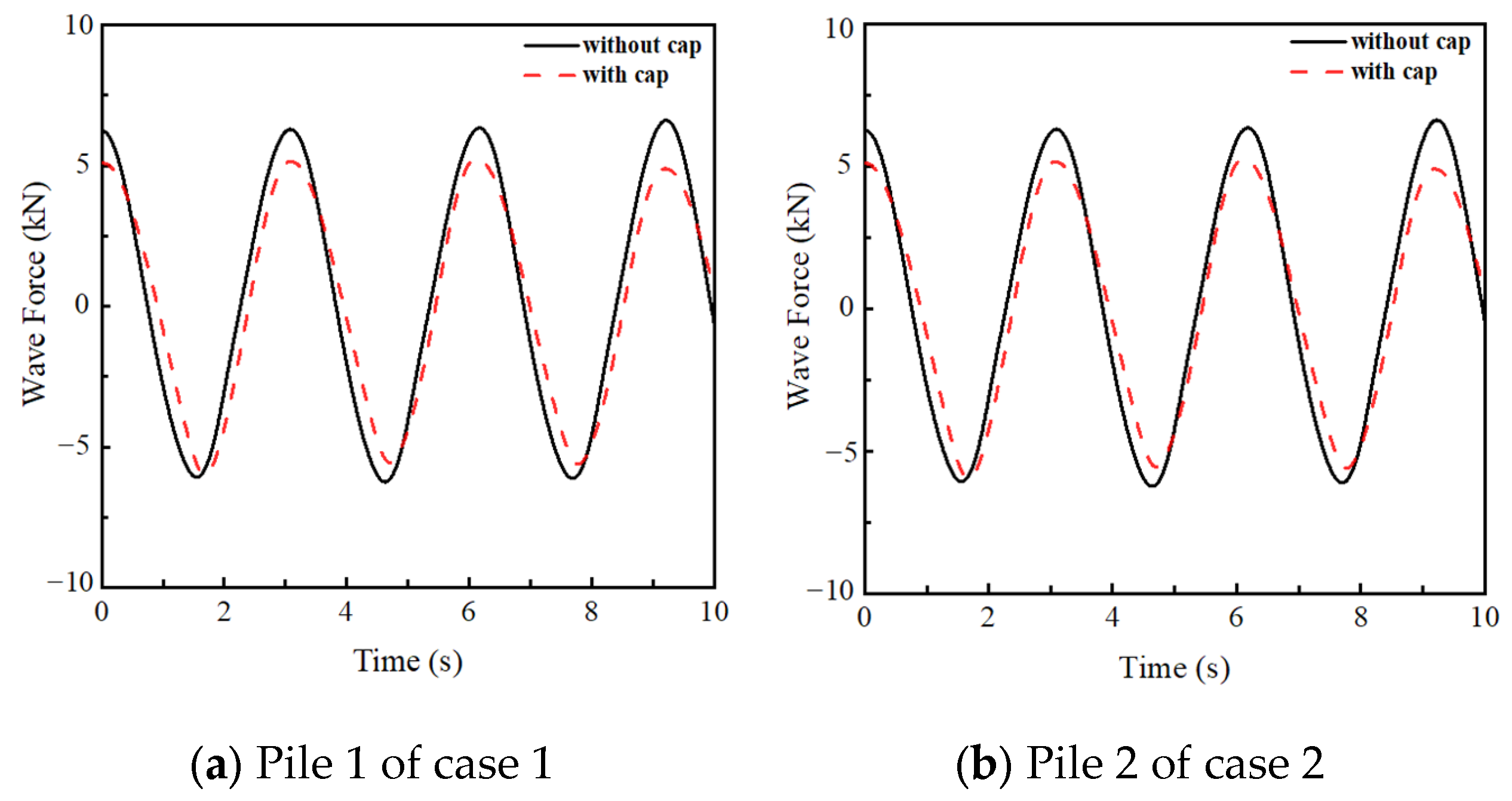
In this paper, a three-dimensional numerical wave flume is established to investigate the influence of the cap on wave forces acting on pile groups. The setup of the flume, including wave generation and elimination, the grid size, and the boundary conditions, has been validated with the test results of the physical flume in the relevant literature. The influence of the cap on the pile groups with different arrangements and water levels was studied. The cap-interference coefficient $K_{cp}$ was defined, and its variation law was given. It was found that for the single row of piles perpendicular to the wave, the center distance of the pile and the width of the cap have little effect on $K_{cp}$. Meanwhile, for the single row of piles parallel to the wave, the cap length before and after the pile has a negative correlation with $K_{cp}$. The law of multi-row piles is similar to that of single-row piles.

We proposed a modified theoretical formula with $K_{cp}$ for calculating wave forces on piles as a theoretical formula for calculating wave forces considering the cap effects. Based on the parametric analysis mentioned earlier, the recommended value of $K_{cp}$ was given.

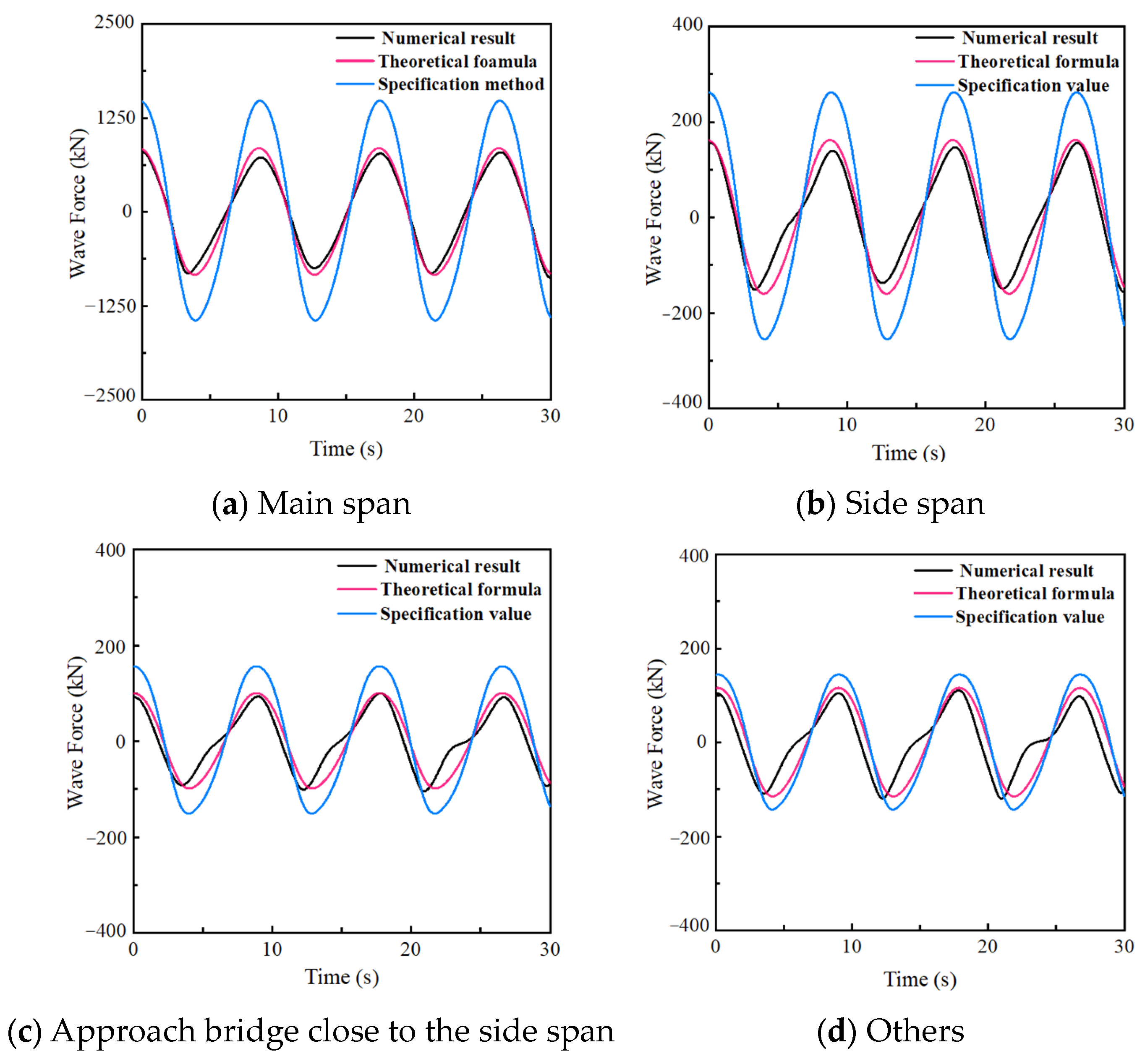
After that, four groups of pile-foundation structures in engineering projects were selected to verify the feasibility of numerical flumes in practical engineering. Comparing the results of the pile-group wave force calculated by the numerical water flume, specification value, and theoretical formula, it is concluded that the results from the numerical water flume are in good agreement with that of the theoretical formula, while the results of the specification value are more conservative. The methods used in this article and the obtained variation laws can provide a reference for engineering.

However, due to limitations in computer power and time, we were unable to calculate many different cases with different sizes of caps, resulting in certain limitations in the formula. At the same time, caps are not only square, but may also have shapes such as circles and triangles, which can be further explored in the future.

References

1. Liu, H. Hydrodynamic Problems Associated with Construction of Sea-Crossing Bridges. J. Hydrodyn. 2006, 18, 13–18. [Google Scholar] [CrossRef]
2. Fang, C.; Tang, H.J.; Li, Y.L.; Wang, Z.W. Effects of random winds and waves on a long-span cross-sea bridge using Bayesian regularized back propagation neural network. Adv. Struct. Eng. 2020, 23, 733–748. [Google Scholar] [CrossRef]
3. Okeil, A.M.; Cai, C.S. Survey of short- and medium-span bridge damage induced by Hurricane Katrina. J. Bridge Eng. 2008, 13, 377–387. [Google Scholar] [CrossRef]
4. Haney, J.P.; Herbich, J.B. Wave Flow around Thin Piles and Pile Groups. J. Hydraul. Res. 1982, 20, 1–14. [Google Scholar] [CrossRef]
5. Fredsoe, J. Turbulent Boundary-Layer in Wave-Current Motion. J. Hydraul. Eng.-Asce 1984, 110, 1103–1120. [Google Scholar] [CrossRef]
6. Kemp, P.H.; Simons, R.R. The Interaction Between Waves and a Turbulent Current—Waves Propagating with the Current. J. Fluid Mech. 1982, 116, 227–250. [Google Scholar] [CrossRef]
7. O’Brien, M.P.; Morison, J.R. The forces exerted by waves on objects. Eos Trans. Am. Geophys. Union 1952, 33, 32–38. [Google Scholar] [CrossRef]
8. Sarpkaya, T. Wave Forces on Offshore Structures; Cambridge University Press: Cambridge, UK, 2010. [Google Scholar]
9. Justesen, P. Hydrodynamic-Forces on Large Cylinders in Oscillatory Flow. J. Waterw. Port Coast. Ocean. Eng.-Asce 1989, 115, 497–514. [Google Scholar] [CrossRef]
10. Sarpkaya, T. Forces on Cylinders near a Plane Boundary in a Sinusoidally Oscillating Fluid. J. Fluids Eng.-Trans. Asme 1976, 98, 499–505. [Google Scholar] [CrossRef]
11. Boccotti, P.; Arena, F.; Fiamma, V.; Barbaro, G. Field experiment on random wave forces acting on vertical cylinders. Probabilistic Eng. Mech. 2012, 28, 39–51. [Google Scholar] [CrossRef]
12. MacCamy, R.C.; Fuchs, R.A. Wave Forces on Piles: A Diffraction Theory; US Beach Erosion Board: San Francisco, CA, USA, 1954. [Google Scholar]
13. Neelamani, S.; Sundar, V.; Vendhan, C.P. Dynamic Pressure Distribution on a Cylinder Due to Wave Diffraction. Ocean Eng. 1989, 16, 343–353. [Google Scholar] [CrossRef]
14. Garrison, C.J.; Chow, P.Y. Wave Forces on Submerged Bodies. J. Waterw. Harb. Coast. Eng. Div. 1972, 98, 375–392. [Google Scholar] [CrossRef]
15. Terro, M.J.; Abdel-Rohman, M. Wave induced forces in offshore structures using linear and nonlinear forms of Morison’s equation. J. Vib. Control 2007, 13, 139–157. [Google Scholar] [CrossRef]
16. Liu, S.X.; Li, Y.C.; Li, G.W. Wave Current Forces on the Pile Group of Base Foundation for the East Sea Bridge, China. J. Hydrodyn. 2007, 19, 661–670. [Google Scholar] [CrossRef]
17. Qu, J.Z.; Xue, L.P.; Wang, B.L.; Ni, X. Unified empirical relations for total inline wave forces on pile-supported structures in regular and irregular waves. Ocean Eng. 2017, 145, 200–206. [Google Scholar] [CrossRef]
18. Zhang, H.C.; Liu, S.X.; Li, J.X.; Fan, Y.P. Experimental study on short-crested random wave interaction with pile group in double-row side-by-side arrangement: A statistical analysis. Coast. Eng. J. 2020, 62, 236–251. [Google Scholar] [CrossRef]
19. Zhang, H.C.; Liu, S.X.; Li, J.X.; Zhang, R.L.; Hao, J. Interactions between multi-directional irregular waves and a pile group in a side-by-side arrangement: Statistical analysis. Coast. Eng. 2019, 147, 115–134. [Google Scholar] [CrossRef]
20. Bonakdar, L.; Oumeraci, H.; Etemad-Shahidi, A. Wave load formulae for prediction of wave-induced forces on a slender pile within pile groups. Coast. Eng. 2015, 102, 49–68. [Google Scholar] [CrossRef]
21. Liu, P.L.F.; Losada, I.J. Wave propagation modeling in coastal engineering. J. Hydraul. Res. 2002, 40, 229–240. [Google Scholar] [CrossRef]
22. Dong, C.M.; Huang, C.J. Generation and propagation of water waves in a two-dimensional numerical viscous wave flume. J. Waterw. Port Coast. Ocean. Eng. 2004, 130, 143–153. [Google Scholar] [CrossRef]
23. Huang, B.; Zhu, B.; Cui, S.G.; Duan, L.L.; Cai, Z.L. Influence of Current Velocity on Wave-Current Forces on Coastal Bridge Decks with Box Girders. J. Bridge Eng. 2018, 23, 04018092. [Google Scholar] [CrossRef]
24. Deng, L.W.; Yang, W.L.; Li, Q.; Li, A. CFD investigation of the cap effects on wave loads on piles for the pile-cap foundation. Ocean Eng. 2019, 183, 249–261. [Google Scholar] [CrossRef]
25. Patankar, S. Numerical Heat Transfer and Fluid Flow; CRC Press: Boca Raton, FL, USA, 2018. [Google Scholar]
26. Prasad, D.D.; Ahmed, M.R.; Lee, Y.H.; Sharma, R.N. Validation of a piston type wave-maker using Numerical Wave Tank. Ocean Eng. 2017, 131, 57–67. [Google Scholar] [CrossRef]
27. Finnegan, W.; Goggins, J. Numerical simulation of linear water waves and wave-structure interaction. Ocean Eng. 2012, 43, 23–31. [Google Scholar] [CrossRef]
28. Orszag, S.A.; Yakhot, V. Renormalization group analysis of turbulence. In Proceedings of the International Congress of Mathematicians, Berkeley, CA, USA, 3–11 August 1986. [Google Scholar]
29. Koushan, K.; Krasilnikov, V.; Nataletti, M.; Sileo, L.; Spence, S. Experimental and Numerical Study of Pre-Swirl Stators PSS. J. Mar. Sci. Eng. 2020, 8, 47. [Google Scholar] [CrossRef]
30. Hirt, C.W.; Nichols, B.D. Volume of Fluid (Vof) Method for the Dynamics of Free Boundaries. J. Comput. Phys. 1981, 39, 201–225. [Google Scholar] [CrossRef]
31. Schlichting, H.; Gersten, K. Boundary-Layer Theory; World Book Publishing Company: Chicago, IL, USA, 2017. [Google Scholar]
32. Mo, W.H.; Irschik, K.; Oumeraci, H.; Liu, P.L.F. A 3D numerical model for computing non-breaking wave forces on slender piles. J. Eng. Math. 2007, 58, 19–30. [Google Scholar] [CrossRef]
33. Xiang, T.; Istrati, D. Assessment of Extreme Wave Impact on Coastal Decks with Different Geometries via the Arbitrary Lagrangian-Eulerian Method. J. Mar. Sci. Eng. 2021, 9, 1342. [Google Scholar] [CrossRef]
34. Celebi, M.S.; Kim, M.H.; Beck, R.F. Fully nonlinear 3-D numerical wave tank simulation. J. Ship Res. 1998, 42, 33–45. [Google Scholar]
35. Romate, J.E. Absorbing Boundary-Conditions for Free-Surface Waves. J. Comput. Phys. 1992, 99, 135–145. [Google Scholar] [CrossRef]
36. Fenton, J.D. The Numerical-Solution of Steady Water-Wave Problems. Comput. Geosci. 1988, 14, 357–368. [Google Scholar] [CrossRef]
37. Wang, Z.G.; Qiu, W.L. Characteristics of wave forces on pile group foundations for sea-crossing bridges. Ocean Eng. 2021, 235, 109299. [Google Scholar] [CrossRef]
38. Xie, S.L.; Shao, S.L.; Zhang, S.H. Code of Hydrology for Sea Harbour; Communications Press Corporation Limited: Beijing, China, 2013. [Google Scholar]
Figure 1. Diagram of the VOF method.
Jmse 11 01677 g001
Figure 2. The grid of the D / 100 boundary layer.
Jmse 11 01677 g002
Figure 3. Simulation results of different boundary layer thicknesses.
Jmse 11 01677 g003
Figure 4. Wave flume test device [32].
Jmse 11 01677 g004
Figure 5. Three-dimensional numerical flume of verification test.
Jmse 11 01677 g005
Figure 6. Local diagram of mesh.
Jmse 11 01677 g006
Figure 7. Schematic diagram of the numerical water flume.
Jmse 11 01677 g007
Figure 8. Comparison of pressure and wave force time history in test and numerical simulation.
Jmse 11 01677 g008
Figure 9. Meshing diagram and numerical flume diagram of capped pile group.
Jmse 11 01677 g009
Figure 10. Comparison of wave-force time history of two piles arranged in the vertical wave direction with or without pile cap.
Jmse 11 01677 g010
Figure 11. The variation of the interference coefficient of the cap with the length of the cap at the back of the pile.
Jmse 11 01677 g011
Figure 12. The variation of the interference coefficient of the cap with the length of the cap in the front of the pile.
Jmse 11 01677 g012
Figure 13. The wave distribution contour along the wave-direction section of pile 1 in the simulation.
Jmse 11 01677 g013
Figure 14. Comparison of wave-force time history of two piles arranged in vertical wave direction at different water levels.
Jmse 11 01677 g014
Figure 15. Geographical location of the bridge.
Jmse 11 01677 g015
Figure 16. Schematic diagram of pile-group foundation.
Jmse 11 01677 g016aJmse 11 01677 g016b
Figure 17. Wave height distribution (m).
Jmse 11 01677 g017
Figure 18. Numerical wave flume of the main span.
Jmse 11 01677 g018
Figure 19. Meshing of the main span.
Jmse 11 01677 g019
Figure 20. Comparison of wave-force time history.
Jmse 11 01677 g020