Underwater Image Enhancement Based on Hybrid Enhanced Generative Adversarial Network

Abstract

In recent years, underwater image processing has played an essential role in ocean exploration. The complexity of seawater leads to the phenomena of light absorption and scattering, which in turn cause serious image degradation problems, making it difficult to capture high-quality underwater images. A novel underwater image enhancement model based on Hybrid Enhanced Generative Adversarial Network (HEGAN) is proposed in this paper. By designing a Hybrid Underwater Image Synthesis Model (HUISM) based on a physical model and a deep learning method, many richly varied paired underwater images are acquired to compensate for the missing problem of underwater image enhancement dataset training. Meanwhile, the Detection Perception Enhancement Model (DPEM) with Perceptual Loss is designed to transfer the coding knowledge in the form of the gradient to the enhancement model through the perceptual loss, which leads to the generation of visually better and detection-friendly underwater images. Then, the synthesized and enhanced models are integrated into an adversarial network to generate high-quality underwater clear images through game learning. Experiments show that the proposed method significantly outperforms several state-of-the-art methods both qualitatively and quantitatively. Furthermore, it is also demonstrated that the method can improve target detection performance in underwater environments, which has specific application value for subsequent image processing.

1. Introduction

Based on the complex microorganisms contained and the scattering phenomenon of light absorption and propagation in the marine water body [1], the acquisition of clear underwater images has become extremely difficult. However, acquiring clear underwater images is useful for surveying marine resources, inspecting marine engineering, defence and military reconnaissance, etc.

High-quality underwater images are often obtained by algorithmic enhancement of the original blurred image, so underwater image synthesis methods were derived to obtain data for underwater image enhancement training. Existing methods for underwater image synthesis include physical model-based, deep learning methods [2,3]. Physical model-based methods usually simulate underwater images with the help of a model to evaluate medium transmission parameters and a priori information. Deep learning approaches usually incorporate neural networks to fit many underwater data parameters to model image details. These methods achieve significant results but have shortcomings. Physical model-based methods rely on specific models and are affected by the diversity of the ocean water column, which absorbs light more severely in water than in the atmosphere, resulting in poorly simulated underwater images. Deep learning-based methods require a lot of training data to generate realistic underwater images.

In addition, high-quality underwater image acquisition cannot be separated from underwater image enhancement technology. Early underwater image enhancement used the polarizer method, which assisted in removing the scattering effect underwater through hardware devices. Nevertheless, it could not solve the problem of underwater image enhancement from the root. Existing underwater image enhancement methods include methods based on traditional enhancement, physical a priori methods, and deep learning methods [4]. Traditional enhancement-based methods process degraded images by adjusting pixel values to improve image quality. Physical a priori-based methods utilize the characteristics of underwater imaging to establish a physical model and estimate the model parameters inversely to derive a clear image based on the assumptions of the a priori conditions. Deep learning methods train the enhanced image by designing the network structure.

Significant progress has been made with these methods, but modelling image distortion due to underwater backscatter with light absorption remains a challenge. Traditional enhancement methods do not apply to marine environments, hardly solving the image degradation problem directly. Physical a priori methods must supplement much of a priori knowledge that relies on accurate environmental information. Deep learning methods do not rely on physical a priori information but require a large amount of data for training due to their black-box nature. In addition, their generalization ability is affected by the marine environment.

To address the above problems, a Hybrid Enhanced Generative Adversarial Network (HEGAN) based on CycleGAN is proposed in this paper. In order to obtain a large number of paired underwater image datasets, a Hybrid Underwater Image Synthesis Model (HUISM) for underwater image synthesis is proposed, which integrates physical modelling and deep learning methods to help the model to complete the degradation process and details of underwater images. To bring the designed image enhancement method closer to reality and to address the problem of effectively improving underwater target detection accuracy with separate underwater image processing, a Detecting Perceptually Enhanced Model (DPEM) is proposed, which includes two kinds of One-stage Deep Detection Perceptors (ODDPs), which transfer the coding knowledge in the form of gradient through perceptual loss to the enhancement model, respectively, to guide the enhancement model to generate images that are visually good and conducive to detection. Finally, HUISM and DPEM are used as generators in HEGAN, which are trained using adversarial loss function and cyclic consistency loss function and eventually generate high-quality and clear images.

The details of the main contributions are given below:

• A Hybrid Underwater Image Synthesis Model (HUISM) is proposed, whose diversity and accuracy for underwater synthesized images are analyzed.
• A Detecting Perceptually Enhanced Model (DPEM) is proposed. Two perceptual loss functions based on patches and target focus detection are designed for the detection perceptron. In addition, the effectiveness of the two detectors is experimentally analyzed.
• A Hybrid Enhanced Generative Adversarial Network (HEGAN) based on CycleGAN is proposed, the effectiveness of which is verified by comparing it with other mainstream methods.

The rest of the paper is structured as follows; Section 2 introduces the related work on underwater image synthesis and enhancement. Section 3 shows the general framework of this paper and the proposed model of the related method. Section 4 presents datasets and experiments. Conclusions are made in Section 5.

2. Related Work

2.1. Underwater Image Synthesis Model

Underwater Image Synthesis (UIS) methods usually form a simulated underwater distorted image after degradation effect operations (e.g., blurring, uneven brightness, low saturation, etc.) on a clear image over water. The main underwater image synthesis methods are physical model-based and deep learning methods.

Physical model-based methods. Since seawater absorbs light and the degree of attenuation is affected by the wavelength of light, most of the degraded images underwater show degraded characteristics of blue-green colour distortion; in addition, seawater scatters light propagation, making the images imaged underwater have the characteristics of lower contrast, fog effect, and so on. Physical model-based methods are usually modelled by the above principles. Guo et al. synthesized an underwater image dataset using 10 Jerlov water types considering depth, wavelength attenuation coefficients, and other parameters for modeling [2]. Georg et al. generated the VAROS synthetic underwater dataset by building a realistic computer graphic model of a large-scale underwater environment, modelling based on the absorption-scattering parameters of light from the water column [5]. In addition, Ueda et al. combined the spectral response of the camera to produce more accurate synthetic images [6].

In recent years, these models have been found to have ignored some critical factors in the underwater imaging process in practice [7,8]. The attenuation coefficient for backscattering is heavily dependent on the obscuring light; thus, the absorption in water is more severe than in the atmosphere. Additionally, the broadband attenuation coefficients for the direct and scattering components are not comparable, and the models are designed to be used a priori on estimating the image transmitted by the scene rather than on estimating the optical properties.

Deep learning methods. With the proposal of Generative Adversarial Networks [9], researchers have focused on transforming overwater and underwater images. Zhao et al. used a jointly trained generative adversarial network for underwater image synthesis and depth map estimation to synthesize realistic underwater images by transferring RGB-D images to multi-style underwater images while preserving object and structural information from aerial images [3]. Zhu et al. designed a CycleGAN network that does not require image pairs and uses an aligned image pair training set to learn the mapping between the input image to the output image, which includes a generator primarily responsible for synthesizing the transformation of an overwater image into an underwater image [10].

This paper combines the advantages of the two methods to design a Hybrid Underwater Image Synthesis Model, which fuses a physical model with a Convolutional Neural Network (CNN) to help the model simulate the degradation process of an underwater image through the physical prior. The CNN is used as a complement to help the model generate more details of the degraded underwater image.

2.2. Underwater Image Enhancement Model

Underwater Image Enhancement (UIE) methods are equivalent to the inverse transformation of UIS, which improves the quality, clarity and visualization of underwater images through a series of operations by modifying the pixel values as well as the depth information of the degraded underwater images, mainly including methods based on traditional enhancement, physical a priori methods, and deep learning methods.

Conventional enhancement methods improve visualization by adjusting the pixel values of an image, which is not fully applicable to a wide range of degradation problems in multiple underwater scenes. Similarly, physical a priori methods rely on a specific model structure. However, the variability of the relevant parameter information required for modelling results in poor image enhancement using physical models alone. Deep learning approaches consider supervised learning in an integrated manner and improve the network to improve image enhancement clarity by training a large amount of data to learn to operate on images with anti-degradation effects. Among them, the GAN enhancement method utilizing a generator and discriminator for game learning attracts wide attention. Zhang et al. introduced the ResNet group on top of the GAN structure. They used its pre-activation to improve the generalization ability as well as the computational efficiency of the model  [11]. Chen et al. proposed UMGAN, which transforms a turbid underwater image to a clear image and adaptively enhances local regions of the image along with global enhancement through Global-Local Discriminators structure [12].

In recent years, researchers have focused on integrating traditional augmentation, physical a priori, and deep learning methods. Huang et al. proposed an underwater contrast enhancement method based on dual-image wavelet transform and GAN, which connects the recovered chrominance channel with the fused luminance channel to obtain high-quality images [13]. Xue et al. jointly predicted underwater degradation factors based on a multi-branch multivariate network to achieve simultaneous image colour correction and contrast enhancement, compensating for image colour and removing the veil [14]. Shi et al. proposed an attention mechanism residual module for colour correction based on the a priori information that both the underwater red and green channels cause colour distortion, with a combination of CLAHE and gamma algorithms to enhance the image [15].

Therefore, this paper proposes a Hybrid Enhanced Generative Adversarial Network based on CycleGan [10], which follows the underwater image synthesis and enhancement model as a generator in two paths, respectively, trained using the adversarial loss function and the cyclic consistency loss function, enabling the overall model to generate high-quality and clear images.

3. Proposed Method

In this section, the corresponding contiguous generative models HUISM and DPEM in HEGAN are first introduced. Then, the corresponding loss functions in their HEGAN are constructed.

3.1. Hybrid Underwater Image Synthesis Model

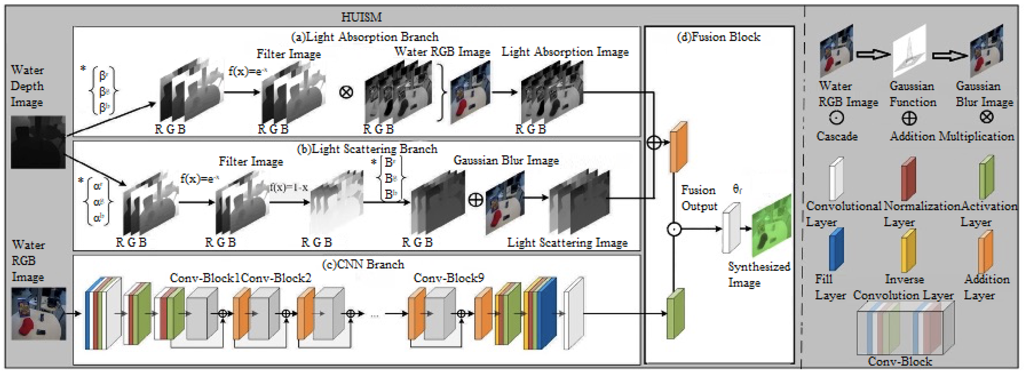
This section proposes a hybrid underwater image synthesis model (see Figure 1), including four modules: (a) Light Absorption Module (LA), (b) Light Scattering Module (LS), (c) CNN Module (CNN), (d) Fusion Module, Fusion. Firstly, applying the a priori knowledge of light absorption and scattering to model the degradation features of underwater images is proposed. Then, a convolutional neural network is utilized to complement the physical model to simulate other degradation details of the underwater image. LA and LS are built based on optical a priori information to form a complete physical model and perform elemental operations with the CNN throughout the whole network, producing an acceptable result as an output.

Light Absorption module. LA aims to simulate the distortion effect of underwater images through the principle of light absorption. Since the degree of light absorption is affected in proportion to the length of the optical path, i.e., light absorption is related to the scene’s depth. Therefore, the light absorption module leads from the depth map over water and can be expressed as:

$$I_{ab}^{\lambda }=I_a^{\lambda }\otimes e^{-I_d{\beta }_{\lambda }},\lambda \in \left\{R,G,B\right\}$$

(1)

where $I_{ab}^{\lambda }$ and $I_a^{\lambda }$ denote the light absorption map as well as the clear RGB map on the water, respectively. $I_d$ shows the depth map on the water with the depth information d, and $\beta$ presents the absorption coefficients of different channels of the RGB image on the water. The ⊗ are the symbols for element-level multiplication operations.

First, the corresponding transition map T is obtained according to the transition equation (Equation (1)):

$$T=e^{-I_d{\beta }_{\lambda }},\lambda \in \left\{R,G,B\right\}$$

(2)

Then, the transition map is multiplied by the information of the three channels of the RGB map on the water to obtain the information of the image after the light absorption degradation effect.

Light Scattering module. LS aims to simulate the blurring effect of underwater images through the principle of light scattering. Light scattering $I_{sc}^{\lambda }$ underwater can be divided into forward scattering $I_{fsc}^{\lambda }$ and backward scattering $I_{bsc}^{\lambda }$. The LS module can be stated as follows:

$$I_{sc}^{\lambda }=I_{bsc}^{\lambda }+I_{fsc}^{\lambda },\lambda \in \left\{R,G,B\right\}$$

(3)

Forward scattering refers to the scattering of light from the imaging device to the underwater scene in the collision process with aquatic organisms. This phenomenon can be well modelled using the Gaussian fuzzy function, representing the fog-like effect caused by forward scattering. On the other hand, backward scattering refers to the scattering of light from the imaging device to the underwater scene after it interacts with the surface of the scene again. Therefore, it can be indicated explicitly as:

$$\left\{\begin{array}{ccc}{I}_{bsc}^{\lambda }=B^{\lambda }\left(1-e^{-I_d{\alpha }^{\lambda }}\right),\hfill & \hfill & \lambda \in \{R,G,B\}\hfill \\ I_{fsc}^{\lambda }=I_a^{\lambda }\delta (x,y),\hfill & \hfill & \lambda \in \{R,G,B\}\hfill \end{array}\right.$$

(4)

where $\alpha$ and B denote the background light coefficient and backscattering coefficient of different channels of the RGB image on water, respectively. The $\delta (x,y)$ can be expressed as the Gaussian function:

$$\left\{\begin{array}{c}\delta (x,y)=A{e}^{-\frac{x^2+y^2}{{\sigma }^2}}\hfill \\ \int \int A{e}^{-\frac{x^2+y^2}{{\sigma }^2}}dxdy=1\hfill \end{array}\right.$$

(5)

CNN module. The CNN complements the physical model consisting of LA and LS and is designed to simulate other more over-degraded details. There are other factors, based on the physical model, to consider, such as the presence of artificial light leading to uneven illumination on the image, motion of the imaging device will introduce noise in the captured image. Based on the fact that the physical model cannot be simulated, this section is refined and supplemented by the CNN module, which is used to construct a deep and densely connected network structure by using nine convolutional blocks stacked together to improve the feature representation capability of the deep network, learn more complex features and patterns, generate more fine-grained colour distortions, illumination variations, and noise.

Fusion module. Fusion aims to fuse physical model branches with CNNs. Its specific expression is as follows:

$$I_{sw}^{\lambda }\left(x,y\right)=\sum _{w=0}^W\sum _{h=0}^H\sum _{m=0}^M{I}_{con}\left(x+w,y+h,m\right){\theta }_f^{\lambda }\left(w,h,m\right),\lambda \in \{R,G,B\}$$

(6)

where $I_{sw}(x,y)$ denotes the pixel value at each pixel point $(x,y)$ of the synthesized image, and ${\theta }_f^{\lambda }$ shows the convolutional filter of size $(W,H,W)$, which is responsible for converting the outputs of the three branches into the three channels of information of the synthesized image. The $I_{con}$ as the fused output of the three branches is denoted as follows:

$$I_{con}=\left(I_{ab}+I_{sc}\right)\odot I_{cnn}$$

(7)

where $I_{cnn}$ presents the output of the CNN module, and ⊙ is the channel-level concatenation operation.

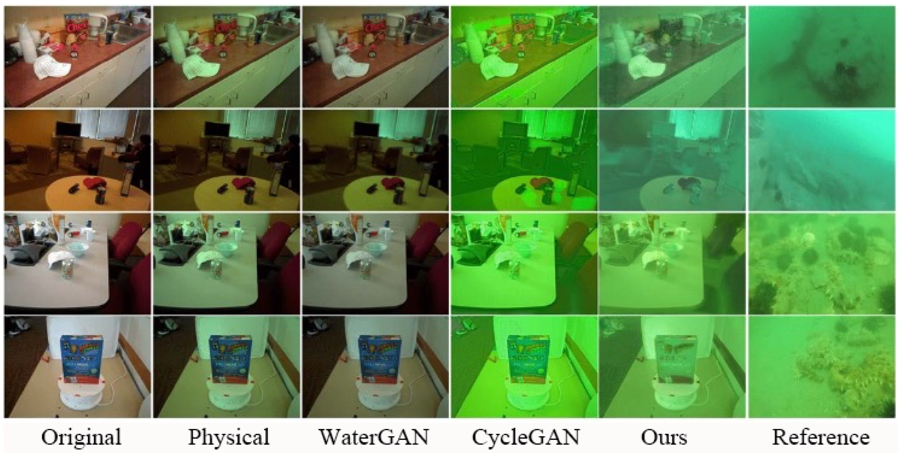
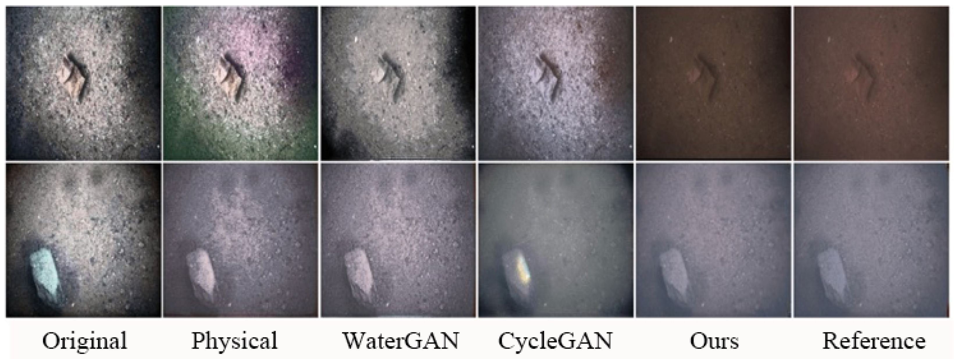
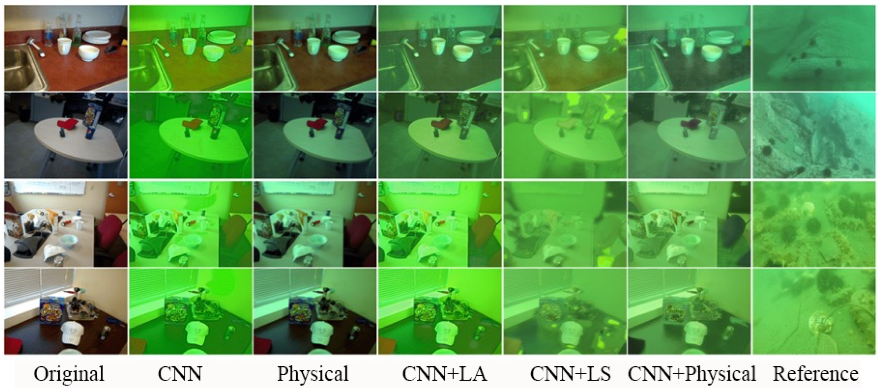
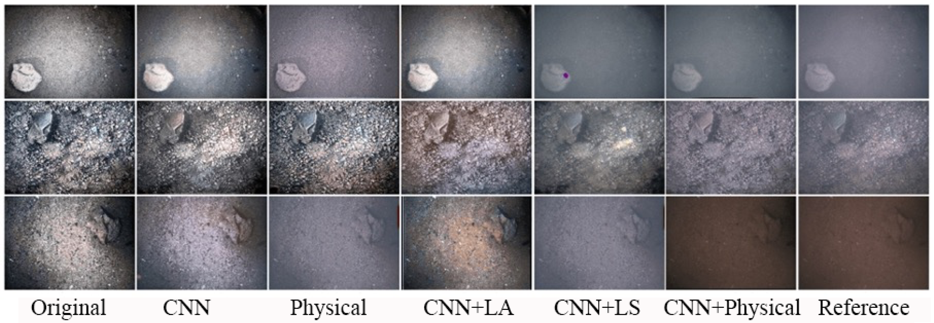
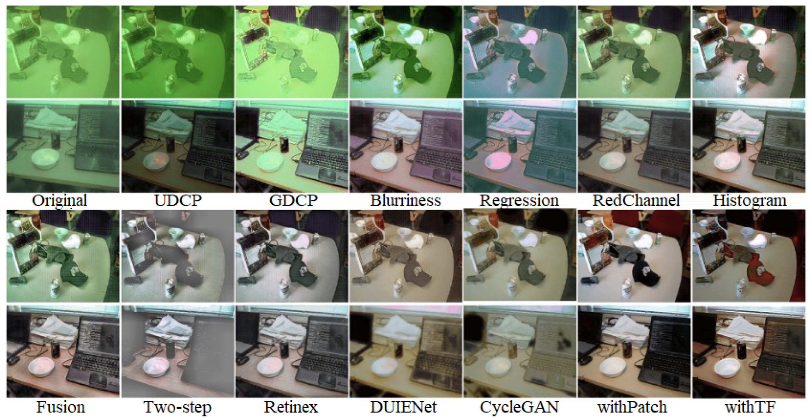
In this paper, this HUISM algorithm is applied to underwater images. Figure 2 and Figure 3 show the visual comparison of some of the synthesized effects (Physical, WaterGAN, CycleGAN, Ours) under Multiview dataset and OUC dataset. Ablation experiments were performed in Section 4.5 to compare the effects of each branch.

3.2. Detecting Perceptually Enhanced Model

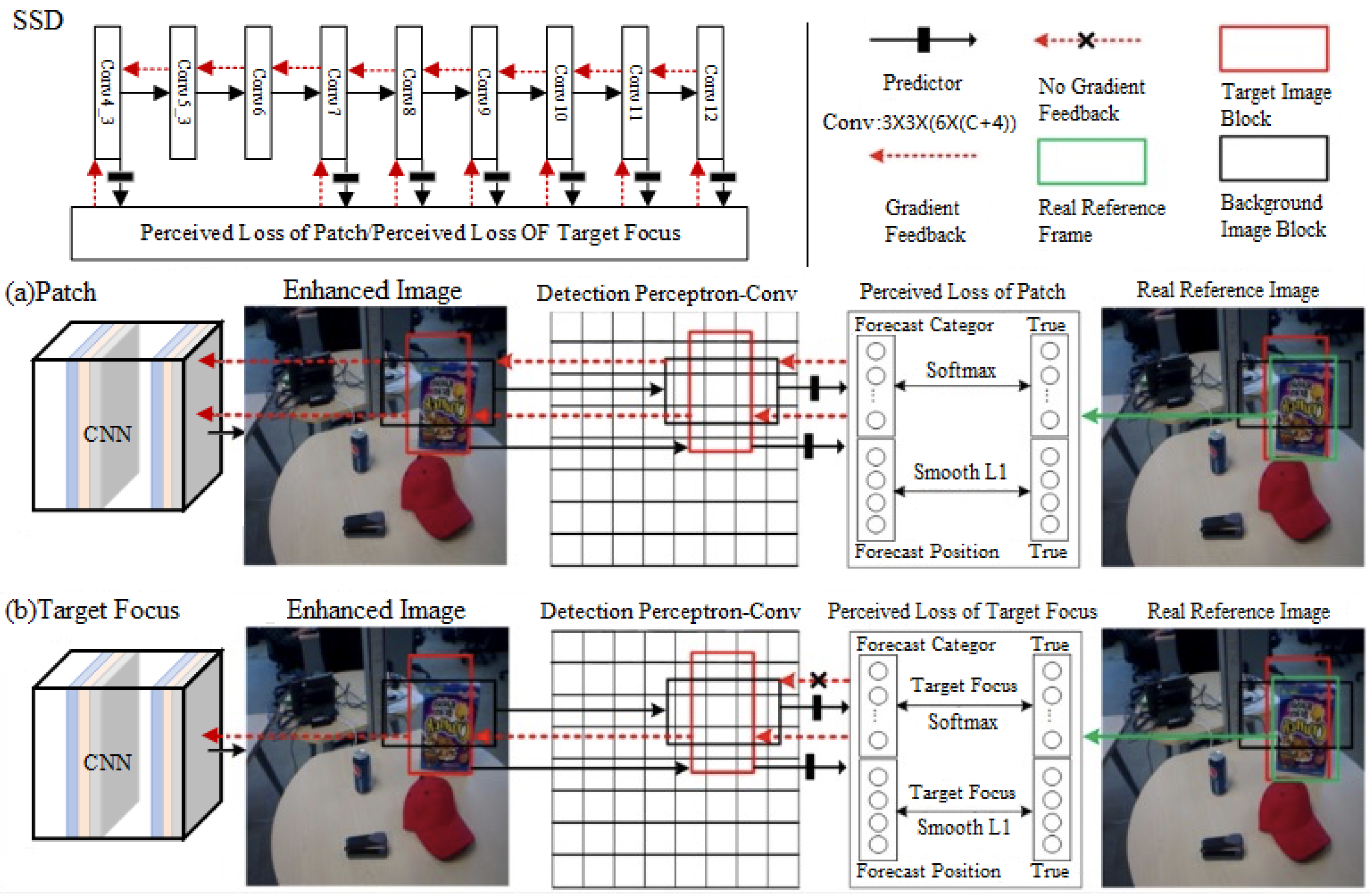
In this section, a Detecting Perceptually Enhanced Model (DPEM) is designed (see Figure 4). First, two detection perceptrons designed based on the perceptual loss function are introduced, and then the image enhancement and the subsequent target detection are regarded as interactive tasks rather than separate individuals.

Based on the properties of the single-stage target detector of the SSD network [16] and its grasp of multi-scale features, it is therefore combined as a detection perceptron, whose specific loss function algorithm, shown in Algorithm 1, provides practical perceptual information for the enhancement model in the subsequent adversarial training (see Section 3.3), the augmented image is directly transmitted to the detection perceptron. First, the image undergoes a CNN module (as a preliminary enhancement model, consistent with the CNN module described in Figure 1) to generate an enhanced clear image, then the detection perceptron associates six default patches with different scales and aspect ratios in the convolutional layer of the SSD model ( simply, Figure 4 describes only two default patches in one of the convolutions), and makes a 3 × 3 convolutional kernel assigning four-dimensional position vectors to the patches, and at the same time, increases the category vectors in the dimensions of the background class number on top of the original number of object classes. Next, the reference classes and positions are determined according to the conditional matching rule of the intersection and concurrency ratio ($IoU$) between the default plaque and its overlapping reference objects as follows:

$$\left\{\begin{array}{ccc}\mathrm{Object}\mathrm{Patch}\mathrm{Category},\mathrm{Location},\hfill & \hfill & \mathrm{If}\mathrm{Results}\in IoU>0.5\hfill \\ \mathrm{Background}\mathrm{Patch},\mathrm{No}\mathrm{Location},\hfill & \hfill & \mathrm{If}\mathrm{Results}\notin IoU>0.5\hfill \end{array}\right.$$

(8)

Finally, the difference between the augmented image patch and the actual reference image patch is computed by the perceptual loss of the detector, and its parameters are constantly updated to feed the difference back to the convolutional neural network model in the form of a gradient. This means the real over-water image scene is encoded into the detection perceptron space before the image enhancement operation. The water image is appropriately transformed to enhance the detailed information of the target in the water and to extract favourable information relevant to the target detection task. This processing can help the augmented model to better detect targets in complex over-water scenes and improve the accuracy and stability of the detection.

Algorithm 1 SSD Loss
$y_{true}\leftarrow True\_Classification\_Data$
$y_{pred}\leftarrow Predicted\_Classification\_Data$
$neg\_pos\_ratio\leftarrow 3.0$
$n\_neg\_min\leftarrow 0$
$\alpha \leftarrow 1.0$
$batch\_size\leftarrow y_{pred}[batch\_size]$
$n\_boxes\leftarrow y_{pred}[n\_boxes]$	▹ Total number of boxes per image
${\mathcal{L}}_{classification}\leftarrow Softmax\_log\_loss(y_{true},y_{pred})$
${\mathcal{L}}_{localization}\leftarrow Smooth\_L1\_loss(y_{true},y_{pred})$
$negatives\leftarrow y_{true}\left[negatives\right]$
$positives\leftarrow y_{true}\left[positives\right]$
$n\_positive\leftarrow \sum positives$
$pos\_class\_loss\leftarrow \sum ({\mathcal{L}}_{classification}\times positives)$
$neg\_class\_loss\_all\leftarrow {\mathcal{L}}_{classification}\times negatives$
$n\_neg\_losses\leftarrow count\_nonzero(neg\_class\_loss\_all)$	▹ Function $count\_nonzero\left(M\right)$ calculate nonzero items number in M
if $neg\_pos\_ratio\times n\_positive\ge n\_neg\_min$ then
$n\_negative\_keep\leftarrow n\_neg\_min$
else
$n\_negative\_keep\leftarrow neg\_pos\_ratio\times n\_positive$
end if
if $n\_negative\_keep\le n\_neg\_losses$ then
$n\_negative\_keep\leftarrow n\_neg\_losses$
end if
if $P=1$ then
if $n\_neg\_losses=0$ then
$neg\_class\_loss=zeros(batch\_size)$	▹ Patch
else
$neg\_class\_loss\leftarrow \sum (L_{classification}\times negative\_keep)$
end if
else
$neg\_class\_loss\leftarrow 0$	▹ Target Focus
end if
${\mathcal{L}}_{cls}\leftarrow pos\_class\_loss+neg\_class\_loss$
${\mathcal{L}}_{loc}\leftarrow \sum ({\mathcal{L}}_{localization}\times positives)$
if $n\_positive\ge 1.0$ then
${\mathcal{L}}_{total}\leftarrow ({\mathcal{L}}_{cls}+\alpha {\mathcal{L}}_{loc})/n\_positive$
else
${\mathcal{L}}_{total}\leftarrow ({\mathcal{L}}_{cls}+\alpha {\mathcal{L}}_{loc})$
end if
${\mathcal{L}}_{total}\leftarrow {\mathcal{L}}_{total}\times batch\_size$

As a result, the final output image after DPEM generates targeted enhanced images based on the different perceptual losses used to serve subsequent advanced visual processing tasks.

Perceptual loss function based on patch detection. The perceptual loss $L_p$ with patch is designed to guide the convolutional neural network model to generate images closer to the exact location, i.e., to generate clear images at the patch level, with the following expression:

$$L_p=\frac{1}{N}\sum _{\begin{array}{c}i\in \mathrm{all}\end{array}}{L}_{cls}\left({pcls}^i,{gcls}^i\right)+\frac{1}{\overline{N}}\sum _{\begin{array}{c}i\notin \mathrm{bg}\end{array}}{L}_{loc}\left({ploc}^i,{gloc}^i\right)$$

(9)

$L_p$ is the weighted sum of the classification loss $L_{cls}$ and the location loss $L_{loc}$. Where ${pcls}^i$ and ${gcls}^i$ denote the predicted and true category vectors of the ith default patch, respectively. Similarly, ${ploc}^i$ and ${gloc}^i$ denote the predicted and true position vectors of the ith default patch, $all$ denotes the set of all default patches, including the set of all target patches versus the set of background patches $bg$, and N and $\overline{N}$ denote the number of all default patches versus the number of target patches, respectively. The specific expressions for classification loss and location loss are as follows:

$$\left\{\begin{array}{c}{L}_{cls}\left({pcls}^i,{gcls}^i\right)=-\sum _{\begin{array}{c}c=1\end{array}}^{C+1}pcl{s}_{c}log\left(gcl{s}_c\right)\hfill \\ L_{loc}\left(ploc,gloc\right)=\sum _{\begin{array}{c}l=1\end{array}}^{4}smoot{h}_{L1}\left({ploc}_l-{gloc}_l\right)\hfill \end{array}\right.$$

(10)

The categorization loss function uses the activation function SoftMax Loss, and the location loss function uses the $smoot{h}_{L1}$ function where $pcl{s}_c$ and $gcl{s}_c$ denote the cth element of the predicted and true category vectors, respectively. Where $plo{c}_l$ and $glo{c}_l$ denote the l-th element of the predicted and true position vectors separately.

In summary, the categorical loss function and the positional loss function encourage the enhancement of images in which the category differences and the positional differences between the image plaques and the genuine plaques are minimized. Therefore, the perceptual enhancement model for plaque detection that combines the two loss functions can learn the basic properties of authentic, clear images, guiding the accuracy of the convolutional neural network model with respect to the category and location of the target to be detected in the image, which helps to recover the details of the image plaques.

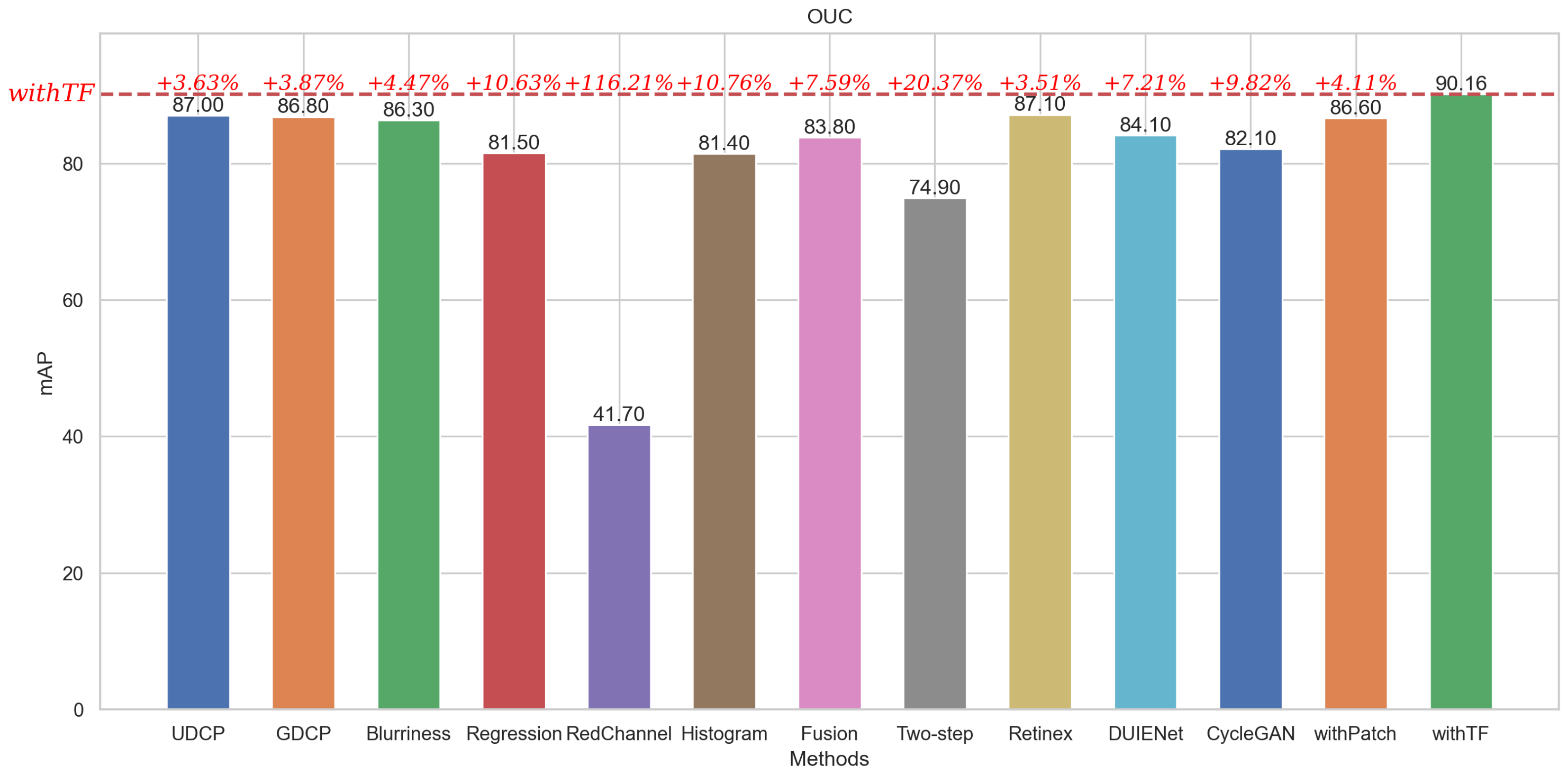
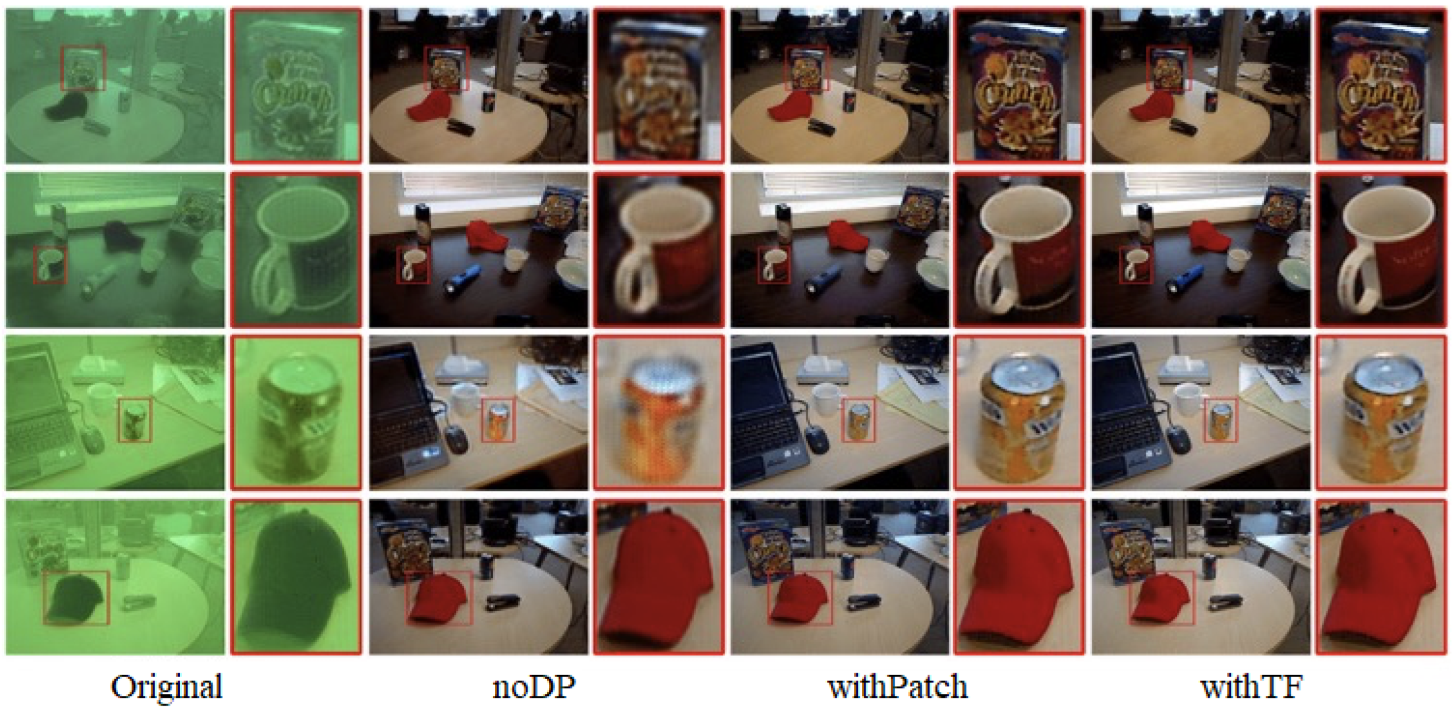
Perceptual loss function based on target focus detection. The perceptual loss $L_{tf}$ of withTF aims to guide the enhancement model to assign the positions of real categories and target frames on the enhanced image to improve the detection accuracy. The complexity of underwater environments leads to the fact that underwater targets to be detected often blend with the background and are difficult to be detected accurately, which becomes a challenging task. To solve this problem, the perceptual loss function of withTF is designed in this section with the following expression:

$$L_{tf}=\frac{1}{\overline{N}}\sum _{\begin{array}{c}i\notin \mathrm{bg}\end{array}}{L}_{cls}\left({pcls}^i,{gcls}^i\right)+L_{loc}\left({ploc}^i,{gloc}^i\right)$$

(11)

The complex background may reduce the detection accuracy of the detector. Therefore, this design only focuses on the feedback target’s patch information and ignores its background patch information. This approach allows the model to dynamically learn regions of the image that are closely related to the target and ignore background information that is not related to the target. This move will improve subsequent detection accuracy (ablation experiments are performed in Section 4.5, demonstrating the superiority of this loss function design).

In summary, the detection perceptual models corresponding to the two perceptual loss functions described above each have their own target points. The perceptual loss function based on patch detection focuses on generating clear images at the patch level, which is more in line with the visual effect of the human eye. The perceptual loss function based on target focus detection focuses on generating salient target images, which enhances the target detection accuracy and better meets the machine vision effect. Therefore, the above characteristics determine that the detection performance of the perceptual model withTF is higher than that of the perceptual model withPatch, whereas the image performance of the perceptual model withPatch is higher than that of withTF (in Section 4.4.1).

3.3. CycleGAN-Based Hybrid Enhanced Generative Adversarial Network

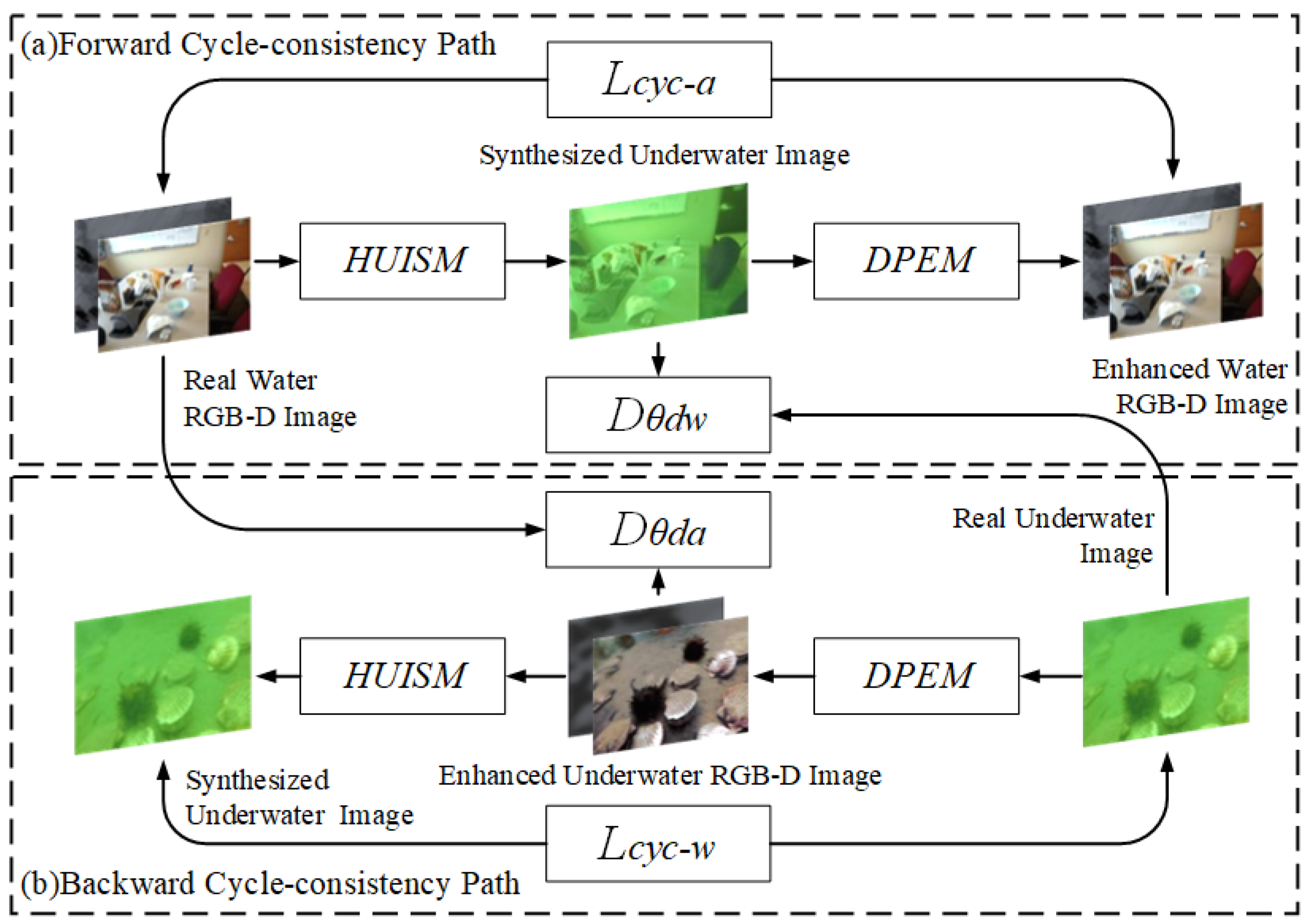
In this section, a Hybrid enhancement generative adversarial network (HEGAN) is designed (see Figure 5). The general framework of the model is first introduced, followed by the design of the loss function for its encounters.

CycleGAN differs from traditional GAN by containing two generators and two discriminators, which realize the role of domain migration, and by learning the mapping relationship between the input domain image to the output domain image, it preserves the specific features of the original domain image while transforming it into an image that satisfies the target output features.

In this section, the CycleGAN structure is improved with the model algorithm shown in Algorithm 2. Among them, the generator includes a synthesis model and an augmentation model, which realize the functions of converting an overwater image to an underwater image, as well as converting an underwater image to an overwater image, respectively. The discriminators discriminate the converted synthetic image and the actual image, respectively. The whole framework will contain two cyclic consistency paths, in which the forward cyclic consistency path starts with the real underwater RGB-D image, generates the synthetic underwater image through HUISM, then generates the enhanced clear underwater RGB-D picture after DPEM as the end point. The reverse cyclic consistency path starts with a real underwater image, then generates an enhanced clear underwater RGB-D picture via DPEM, and finally ends with a reconstructed synthetic underwater image. Specifically, HUISM and DPEM act as model generators to complete the transformation between the underwater and overwater domains learnt from the unpaired images. $D_{\theta dw}$ and $D_{\theta da}$ act as the discriminators of the model (where $D_{\theta dw}$ discriminates the synthetic underwater image from the real underwater image, and $D_{\theta da}$ discriminates the augmented clear underwater RGB-D image from the real over-water RGB-D image) to perform adversarial training together with the generator using adversarial loss and cyclic consistency loss. In addition, during the training period of DPEM, the detection of favourable information is fed back in the form of a gradient through the perceptual loss of target focusing or plate detection to improve the subsequent target detection ability of the formed realistic image.

Corresponding loss function selection based on HUISM. The loss function $L_{a2w}$ corresponding to the HUISM model consists of an adversarial loss function $L_{adv-w}$ and a cyclic consistency loss function $L_{cyc-w}$, which is formulated as follows:

$$L_{a2w}={\omega }_1{L}_{adv-w}+{\omega }_2{L}_{cyc-w}$$

(12)

where $L_{adv-w}$ is the adversarial loss generated by the discriminator $D_{\theta dw}$, parametrically expressed as $\theta dw$. Taking the clear RGB-D image on the water as input, the underwater synthetic image is generated by HUISM, and the discriminator discriminates it from the real underwater image, so that the minimum estimated probability that the discriminator considers the underwater synthetic image to be the real underwater image is $L_{adv-w}$; thus, the specific expression of $L_{adv-w}$ is as follows:

$$L_{adv-w}=-log{D}_{\theta dw}\left(G_{\theta a2w}\left(I_a,I_d\right)\right)$$

(13)

where $G_{\theta a2w}\left(I_a,I_d\right)$ denotes an underwater synthetic image, parametrically expressed as $\theta a2w$.

During the training process, although the use of the adversarial loss function alone can enable the generator to produce sufficiently realistic underwater images, the phenomenon that multiple input images are all mapped to the same output image may occur during the training process, causing the network to crash. Therefore, the introduction of cyclic consistency loss function can effectively solve the problem.

Algorithm 2 Hybrid Enhanced Generative Adversarial Network
$G_{\theta a2w}\leftarrow Forward\_Generator\_(withPatch/TF)$	▹ Initialize cycle generators and discriminators
$G_{\theta w2a}\leftarrow Backward\_Generator\_(withPatch/TF)$
$D_{\theta da}\leftarrow Forward\_Discriminator$
$D_{\theta dw}\leftarrow Backward\_Discriminator$
$I_a\leftarrow Real\_Overwater\_Image$
$I_w\leftarrow Real\_Underwater\_Image$
$S_w\leftarrow G_{\theta a2w}\left(I_a\right)$	▹ Synthesized underwater image
$S_a\leftarrow G_{\theta w2a}\left(I_w\right)$	▹ Enhanced underwater image
$I_a^{\prime }\leftarrow G_{\theta w2a}\left(I_w\right)$	▹ Enhancement model to enhance synthetic underwater image
$I_w^{\prime }\leftarrow G_{\theta a2w}\left(I_a\right)$	▹ Synthesis model for enhanced underwater image
$V_a\leftarrow PerceptorA\left(I_a^{\prime }\right)$	▹ Perceptor feeds the gradient of favorable information back to augmentation model
$Output\leftarrow [I_a^{\prime },I_w^{\prime },D_{\theta dw}\left(S_a\right),D_{\theta da}\left(S_w\right),V_a]$
$Loss\leftarrow [{\mathcal{L}}_{cyc-a},{\mathcal{L}}_{cyc-w},{\mathcal{L}}_{adv-a},{\mathcal{L}}_{adv-w},{\mathcal{L}}_{ssd}]$
$Weight\leftarrow [{\lambda }_1,{\lambda }_2,{\lambda }_D,{\lambda }_D,{\lambda }_P]$
return $Model(Output,Loss,Weight)$

Where $L_{cyc-w}$ denotes the distance between the synthesized underwater image and the real reference image underwater, with the expression:

$$L_{cyc-w}={∥G_{\theta a2w}\left(G_{\theta w2a}\left(I_w\right)\right)-I_w∥}_1$$

(14)

Denotes the Manhattan distance between the synthesized underwater image $I_w$.The cyclic consistency loss function ensures that the generated final image is as realistic as possible while preventing the model from crashing to generate the same image.

Corresponding loss function selection based on DPEM. The loss function $L_{w2a}$ corresponding to the DPEM model consists of an adversarial loss function $L_{adv-a}$, a cyclic consistency loss function $L_{cyc-a}$, and a perceptual loss of withTF $L_{tf}$ (or with Patch $L_p$), which is formulated as follows:

$$L_{w2a}={\omega }_1{L}_{adv-a}+{\omega }_2{L}_{cyc-a}+{\omega }_3{L}_{tf}+{\omega }_4{L}_p$$

(15)

Similarly, $L_{adv-a}$ is the adversarial loss generated by the discriminator $D_{\theta da}$, parametrically expressed as $\theta da$.

Taking the real underwater image as input, the enhanced clear underwater image is generated by DPEM, and the discriminator discriminates it from the real water image, so that the minimum estimated probability for the discriminator to consider the enhanced clear underwater synthetic image as the clear and real reference image on the water is $L_{adv-a}$, which is formulated as follows:

$$L_{adv-a}=-log{D}_{\theta da}\left(G_{\theta w2a}\left(I_w\right)\right)$$

(16)

Similarly, during the training process, although the use of the adversarial loss function alone can enable the generator to produce a sufficiently realistic clear image of the water, it is equally likely that a network crash will occur during the training process. Therefore, the introduction of a cyclic consistency loss function can effectively solve this problem. Therefore, the specific expression of $L_{cyc-a}$ is as follows:

$$L_{cyc-a}={∥G_{\theta w2a}\left(G_{\theta a2w}\left(I_a\right)\right)-I_a∥}_1$$

(17)

where $I_a$ represents the real reference RGB image on water.

4. Experimental and Analysis

4.1. Dataset Construction

ChinaMM-Multiview dataset. The unpaired dataset combines the underwater image dataset ChinaMM [17] and the overwater RGB-D image dataset MultiView [18]. Among them, ChinaMM consists of a training set of 2071 images and a test set of 676 images, including three object categories of sea cucumbers, sea urchins, and scallops, each with a resolution of 720 × 405 pixels. MultiView consists of a training set of 14,179 images and a test set of 1206 images, including five object categories. In this paper, the images in Multiview are randomly selected to constitute the same number of training and test sets as ChinaMM for the unpaired dataset ChinaMM-Multiview, and the resolution of each image is 640 × 480 pixels.

OUC dataset. The underwater OUC dataset [19] consists of a training set of 2500 image pairs and a test level of 1198 image pairs, based on the fact that this dataset does not have a depth map required by the algorithms in this paper, and therefore its corresponding depth images are obtained by the UW-net [20] method.

4.2. Implementation Details

The experimental runtime environment is configured as follows: CPU (Intel Xeon CPU @2.40GHz (Intel, Santa Clara, CA, USA)), GPU (2 parallel NVIDIA Tesla P100 GPUs (NVIDIA, Santa Clara, CA, USA)), the framework is Keras in Python 3.8, where the Adam optimization algorithm is used to set the initial learning rate to 0.0002, which decays linearly after 100 epochs and learning is stopped after 300 epochs.

4.3. Evaluation Indicators

For the evaluation of the enhanced image, MSE, PSNR, SSIM, PCQI, mAP, UIQM, and UCIQE are used for integrated consideration. Where MSE denotes the mean square error, which is expressed as:

$$MSE=\frac{1}{M\times N}\sum _{i=1}^M\sum _{j=1}^N{\left(I(i,j)-N(i,j)\right)}^2$$

(18)

Among them, $I(i,j)$ and $N(i,j)$ denote the image to be evaluated and the reference image, M is the total number of pixels of the image to be evaluated, and N is the total number of pixels of the original image. When the MSE value is lower, the effect of the image to be evaluated is closer to that of the reference image.

Peak Signal to Noise Ratio PSNR is an objective evaluation metric used to evaluate image distortion and is calculated as follows:

$$PSNR=10{log}_{10}\left(\frac{g^2}{\mathrm{MSE}}\right)$$

(19)

where g denotes an image’s total pixel grey value, usually taken as 255, the PSNR unit is dB. When the PSNR value is more prominent, it means the quality of the image is better. Structural similarity SSIM is used to evaluate the level of similarity between two images. For images X and $Yd$, the structural similarity expression is as follows:

$$SSIM\left(X,Y\right)=\frac{\left(2{\mu }_X{\mu }_Y+C_1\right)\left(2{\sigma }_{XY}+C_2\right)}{\left({\mu }_X^2+{\mu }_Y^2+C_1\right)\left({\sigma }_X^2+{\sigma }_Y^2+C_2\right)}$$

(20)

Here, ${\mu }_X$ and ${\mu }_Y$ denote the mean value of X and Y, ${\sigma }_X^2$ and ${\sigma }_Y^2$ denote the variance of X and Y, ${\sigma }_{XY}$ denotes the covariance, and $C_1$ and $C_2$ are constants. SSIM takes the value from 0–1. When it is close to 1, the image to be evaluated is more similar to the reference image and the more similar it is.

The specific expression for the patch-based contrast quality index PCQI [21] is:

$$PCQI(x,y)=q_i(x,y)·q_c(x,y)·q_s(x,y)$$

(21)

It consists of the average intensity $q_i$, the signal strength $q_c$ and the signal structure $q_s$ to evaluate their perceived distortions and can predict spatially localized quality changes. When its value is higher, it indicates better image quality.

The mean average precision mAP is an index to determine the performance of the target detection algorithm, which is the mean value of the average precision AP. The specific formula is as follows:

$$mAP=\frac{{\sum }_{i=1}^{K}A{P}_i}{K}$$

(22)

The expression for AP is:

$$AP=\sum _{i=1}^N{P}_{\mathrm{interp}}\left(r_i\right)\left(r_i-r_{i-1}\right)$$

(23)

where $P_{i}nterp\left(r_i\right)$ denotes the maximum precision of the recall rate value of $r_i$, and N denotes the total number of recall rates of the model prediction statistics.

The evaluation index of underwater image quality, UIQM [22], is based on the color measurement index (UICM), sharpness measurement index (UISM) and contrast measurement index (UIConM), and the specific expression is as follows:

$$UIQM=c_1·UICM+c_2·UISM+c_3·UIconM$$

(24)

UIQM evaluates underwater images’ degradation mechanism and imaging characteristics and can effectively assess underwater image quality based on human perception.

The underwater colour image quality assessment UCIQE utilizes the components of chromaticity $\delta$, saturation $co{n}_l$, and contrast $\mu$ for quantitative assessment to quantify the uneven bias, blurring, and low-contrast situations, respectively. The expression is as follows:

$$UCIQE=c_1·\delta +c_2·co{n}_l+c_3·\mu ,$$

(25)

where c is a constant. Higher values indicate better image quality.

4.4. Evaluation Datasets

4.4.1. Comparison of Evaluation Indicators for Different Datasets

We compare our model with state-of-the-art methods, including six physical model-based methods (UDCP [23], GDCP [24], Blurriness [25], Regression [26], RedChannel [27], and Histogram [28]), three traditional augmentation methods (Fusion [29], Two-step [30], and Retinex [31]), and two deep learning methods (DUIENet [32] and CycleGAN [10]).

Subjective evaluation. For the subjective evaluation, the visual comparison of underwater images using the ChinaMM dataset is shown in Figure 6. In order to investigate the performance of deep learning-based methods on real datasets, the FUnIEGAN [33] and AIOGAN [34] methods were also added to this dataset. The underwater images in the ChinaMM dataset show more serious colour deviations and image distortions by comparison methods (UDCP, GDCP, Blurriness, RedChannel) are unable to address severe color distortions, and the comparative methods (Histogram, Retinex, and deep learning approaches), while effective in handling color deviations, are unable to restore sharpness. The withTF algorithm in our approach significantly enhances the clarity of underwater images, demonstrating superior performance.

A visual comparison of underwater images using the Multiview dataset is presented in Figure 7, revealing that several methods based on physical model correction for distortions yield suboptimal results and may even introduce unsatisfactory colors. The comparison methods (GDCP, Histogram, Retinex) correct the images that are too saturated. Several methods based on deep learning are ineffective in restoring image sharpness. In contrast, the method proposed in this paper effectively resolves the colour bias and image distortion blurring.

A visual comparison of underwater images using the OUC dataset is shown in Figure 8. When the tonal situation changes, the physical-based models are not effective, the deep learning methods are not compatible with both chromatic aberration correction as well as image sharpness, and the traditional enhancement methods are more effective in processing. However, our approaches are still able to better improve the colour bias, saturation, and contrast of the image.

For the objective evaluation, we utilize relevant evaluation metrics to assess various algorithms with the ChinaMM dataset, as presented in

Table 1. Image quality evaluation metrics on ChinaMM dataset (Bold indicates the best value).

Index	UCIQE	UIQM	UICM	UISM	UIConM	mAP
Original	21.2789	1.4379	−79.8641	6.7749	0.4651	68.3
UDCP	28.5643	3.021	−56.7135	6.6857	0.7364	71.5
GDCP	33.6316	2.6415	−53.7259	6.7846	0.6016	72.8
Blurriness	30.5846	3.6978	−58.1637	6.7135	0.9368	77.2
Regression	29.3868	3.7634	−21.9867	6.7059	0.6721	71.5
RedChannel	30.8721	3.3082	−31.2284	6.6944	0.6107	73.8
Histogram	33.3434	4.6782	0.4585	6.7201	0.7428	76.7
Fusion	31.7689	4.0669	−22.2501	6.6552	0.7634	75.6
Two-step	15.1283	2.6782	−4.3982	5.7987	0.3032	58.5
Retinex	28.4741	4.736	−0.4822	6.6715	0.7744	78.7
FUnIEGAN	30.4582	3.6077	−34.2783	6.7472	0.7212	73.6
AIOGAN	30.8543	3.3713	−40.8727	6.6001	0.726	72.7
DUIENet	31.5578	2.7012	−39.4925	6.6224	0.521	71.6
CycleGAN	30.7911	3.7063	6.9858	6.5735	0.4367	67.8
withPatch	32.5967	4.8702	13.9976	6.7362	0.6926	79.4
withTF	32.0976	4.4612	12.4005	6.5322	0.617	83.8

. Although the GDCP method achieves the highest scores in UCIQE and UISM metrics, Blurriness attains the best UIConM metric values. However, both methods fall short in effectively mitigating image distortion effects from a visual perspective. In contrast, the withPatch and withTF algorithms achieve the best values in other metrics and are visually effective in addressing image degradation.

The assessment of different algorithms for underwater images using the Multiview dataset is depicted in

Table 2. Image quality evaluation metrics on MultiviewM dataset (Bold indicates the best value).

Index	MSE	PSNR	SSIM	PCQI	mAP
UDCP	1.0588	18.501	0.1804	0.5436	72
GDCP	3.2652	13.434	0.2709	0.5347	74.2
Blurriness	0.9378	19.631	0.2581	0.5956	74.4
Regression	0.7254	19.912	0.2152	0.5979	71.8
RedChannel	0.7289	20.27	0.4053	0.5993	76.3
Histogram	0.8535	19.193	0.5497	0.5927	78.3
Fusion	1.1393	18.223	0.464	0.5757	77.1
Two-step	2.1466	15.001	0.3721	0.502	66.1
Retinex	0.7315	19.885	0.5231	0.6342	78.3
DUIENet	0.2698	23.876	0.7786	0.6804	76.4
CycleGAN	0.7787	20.752	0.559	0.5585	74.8
withPatch	0.0435	33.3678	0.9347	0.8439	79.9
withTF	0.1638	26.1412	0.6346	0.6714	86.7

. The evaluation of different algorithms for underwater images using the OUC dataset is presented in

Table 3. Image quality evaluation metrics on OUC dataset (Bold indicates the best value).

Index	MSE	PSNR	SSIM	PCQI	mAP
UDCP	3.6174	12.9669	0.487	0.4178	87
GDCP	2.4151	15.7746	0.6361	0.5606	86.8
Blurriness	0.6111	20.9957	0.7293	0.6439	86.3
Regression	0.4249	22.1152	0.5334	0.6602	81.5
RedChannel	7.1875	9.7271	0.1789	0.1649	41.7
Histogram	0.5352	21.3013	0.7513	0.8098	81.4
Fusion	0.2861	28.5391	0.8749	0.8904	83.8
Two-step	1.6224	16.1585	0.618	0.4758	74.9
Retinex	0.3496	28.0591	0.8868	0.8376	87.1
DUIENet	0.1271	27.968	0.8421	0.745	84.1
CycleGAN	0.1316	26.8583	0.8907	0.9344	82.1
withPatch	0.0242	35.4093	0.9742	0.9398	86.6
withTF	0.0661	30.8626	0.9315	0.9003	90.1

. It is evident that the method proposed in this paper attains the highest values for each index in both the Multiview dataset and the OUC dataset, affirming the validity of this algorithm.

4.4.2. Underwater Vision Inspection Algorithm Performance Comparison Analysis

In order to verify that our algorithmic model can be subsequently applied to underwater image-related tasks, we tested the target detection algorithm on images from three datasets, analyzed with respect to the mAP metrics, as shown in Figure 9, Figure 10 and Figure 11.

Among them, withTF achieves the optimal value of the mAP evaluation metrics based on its property of ignoring the background patch information in the default patch while highlighting the category and location information of the target patch. In the ChinaMM dataset, withTF improves the detection accuracy by 43.25% compared with the algorithm Two-step, which has the lowest evaluation value, and improves the detection accuracy by 6.48% compared with the algorithm Retinex, which has the highest evaluation value. In the Multiview dataset, withTF’s value improved by 31.16% compared to the worst algorithm and 10.7% compared to the better algorithm. In the OUC dataset, WithTF achieved a high score of 90.16, which is a 116.21% improvement over the worst algorithm and 3.51% improvement over the better algorithm.

In addition, this paper shows example image visualization results for ChinaMM and Multiview datasets, as shown in Figure 12 and Figure 13. The figure shows the original image, the comparison algorithm, and all the reference images for target detection in the original image.The algorithm proposed in this paper can effectively detect the target object with the best detection results.

4.5. Ablation Study

In this section, we conduct several ablation studies to demonstrate the validity of several components of our model.

Component analysis of HUISM. For HUISM, we tried to test the CNN, LA and LS and the full physics module (consisting of LA and LS) and analyze its role. Figure 14 and Figure 15 show the ablation study under the Multiview and OUC datasets. The effects produced by the CNN alone and the CNN+LA are still clear, while the effects with the LS the synthesized effect is blurred, indicating that light scattering brings a blurring effect to the image. Light absorption produces a different colour tone to the original image, avoiding the artifactual effect of the image. The synthesized effects of CNN and physical modules only have a single style, and the degradation features are all the same. The former is due to the deep learning model pattern collapse problem, and the latter is due to the training optimization of the fixed parameters of the physical model. Once the CNN and physics modules are fused, they form a complementary advantage, making the synthesized effect similar to the reference image.

Objectively speaking, this paper uses evaluation metrics for quantitative comparison, as shown in

Table 4. Quantitative comparison of synthetic models containing different components on the OUC dataset (✓ indicates that the structure was used. Bold indicates the best value).

Model	CNN	LA	LS	MSE	PSNR	SSIM	PCQI
hybrid model	✓	-	-	0.2657	23.3678	0.7563	0.6445
	✓	✓	-	0.1291	26.7168	0.8639	0.9263
	✓	-	✓	0.1301	27.1058	0.9011	0.9307
	-	✓	✓	0.2868	23.7581	0.7564	0.6585
	✓	✓	✓	0.0969	28.2684	0.9167	0.9601

. On the OUC dataset, it can be seen that the complete HUISM outperforms the other choices in MSE, PSNR, SSIM, and PCQI metrics. In situations where LA fails to function correctly, picture artifacts may arise, leading to a decrease in the MSE metric and an increase in the values of the other three metrics. When LS fails to function properly, it results in a picture-blurring phenomenon. This phenomenon can lead to a decrease in MSE metrics and an increase in the values of the other three metrics. HUISM with only a physical or a CNN module will cause MSE metrics to increase and the other three metrics’ values to decrease.

Table 5. Quantitative comparison of different underwater synthesis algorithms algorithms (Bold indicates the best value).

Method	MSE	PSNR	SSIM	PCQI
Physical	0.4305	20.7056	0.6704	0.4827
WaterGAN	0.3211	23.2206	0.7783	0.5619
CycleGAN	0.3701	23.3569	0.7495	0.6483
Ours	0.0987	28.2589	0.9331	0.9505

displays the evaluation of the HUISM method with Physical, WaterGAN and CycleGAN methods under four medium indicators; it is clear that the HUISM method has the lowest MSE evaluation indicator and the highest PSNR, SSIM and PCQI indicators, which indicates that the present method outperforms the other three state-of-the-art methods, and it shows a solid practical value.

In addition, this paper calculates the time complexity of the three branching modules of LA, LS and CNN in HUISM. Referring to Equations (1) and (2), LA module element-level operation is the main factor affecting the running time, and the branching time complexity is denoted as follows:

$$T_1\sim O(W·H·C)$$

(26)

Referring to Equations (3)–(5), the time-consuming computations in the LS module are matrix multiplication and element-level addition, and its branching time complexity is expressed as follows:

$$T_2\sim O(W^2·H·C+W·H·C)$$

(27)

where W, H and C denote the length, width and number of channels of the input image, respectively.

Referring to the CNN module in Figure 1, its time complexity is dominated by the convolutional operations within each layer, and this branching time complexity is analyzed through the evaluation of the work in [35]:

$$T_3\sim O(\sum _{l=1}^D{M}_l^2·K_l^2·C_{l-1}·C_l)$$

(28)

where D is the depth of the network, l is the network layer number, $C_l$ is the number of output channels in the lth layer, $C_{l-1}$ is the number of input channels to the network in the lth layer, and $K_l$ is the edge length of the convolution kernel in the lth layer.

The main time consumption of HUISM comes from the CNN branch, which was found to be true by actually running the program print on CPU (LA:0.0495s, LS:0.0080s, CNN:0.2399s). Thanks to the convenience of keras, this program actually runs on GPU, which greatly reduces the computational time consumption through massive parallelization.

Component analysis of the detector enhancement model. This section compares the enhancement models with three different detector settings (with no detector noDP, patch detector withPatch, and target focusing detector withTF) and analyzes their roles and effects. Figure 16 and Figure 17 show the detection under the ChinaMM and Multiview datasets. The image under noDP still carries the effect of artefacts and distortion; the detected image is still blurred. The image quality under with patch is significantly improved with more explicit details and contours, indicating that the plaque detection enhancement model is capable of paying attention to the image’s subtle features and texture information.

In addition, this paper uses evaluation metrics for quantitative comparison, as shown in

Table 6. Quantitative comparison of different detection perceptron models(Bold indicates the best value).

Method	Multiview					ChinaMM
	MSE	PSNR	SSIM	PCQI	mAP	UCIQE	UIQM	mAP
noDP	0.7135	20.5479	0.5623	0.5668	77.6	27.326	3.8169	76.4
withPatch	0.2435	33.3664	0.9381	0.8438	79.8	32.5867	4.8702	79.4
withTF	0.4676	26.1412	0.6346	0.6737	86.8	28.3296	4.2185	83.8

. WithPatch achieves the best evaluation of image metrics under Multiview and ChinaMM datasets. In contrast, withTF achieves the best evaluation of mAP, which indicates that its enhancement model has excellent potential for subsequent advanced target detection. Moreover, the mAP values of the two detectors under the two datasets are close, demonstrating that the underwater image enhancement effect is similar to the real reference situation of clear images on the water.

5. Conclusions

To address the challenge of insufficient high-quality underwater image data during the training process of underwater image enhancement, we introduce a hybrid underwater image synthesis model. This approach combines both physical modeling and deep learning techniques to accurately represent the degradation process of underwater images. Simultaneously, we establish a hybrid enhancement generative adversarial network (GAN) that incorporates a detection-aware enhancement model. This network facilitates the transformation of images from above-water to underwater domains through an adversarial framework, resulting in the generation of high-quality and clear underwater images. This not only enhances subsequent detection efficiency and accuracy but also addresses various requirements in underwater image processing, including image hue, visibility, saturation, and contrast. Experimental results demonstrate the superior performance of this enhancement algorithm, rendering it well-suited for a range of underwater image processing tasks, notably subsequent target detection in underwater environments.

References

1. Wang, Y.; Song, W.; Fortino, G.; Qi, L.Z.; Zhang, W.; Liotta, A. An experimental-based review of image enhancement and image restoration methods for underwater imaging. IEEE Access 2019, 7, 140233–140251. [Google Scholar] [CrossRef]
2. Guo, Z.; Zhang, L.; Jiang, Y.; Niu, W.; Gu, Z.; Zheng, H.; Wang, G.; Zheng, B. Few-shot fish image generation and classification. In Proceedings of the Global Oceans 2020: Singapore–US Gulf Coast, Singapore, 5–30 October 2020; pp. 1–6. [Google Scholar]
3. Zhao, Q.; Zheng, Z.; Zeng, H.; Yu, Z.; Zheng, H.; Zheng, B. The synthesis of unpaired underwater images for monocular underwater depth prediction. Front. Mar. Sci. 2021, 8, 690962. [Google Scholar] [CrossRef]
4. Vijay Anandh, R.; Rukmani Dev, S.; Preetham, S.; Pratheep, K.; Reddy, P.B.P.; Ram Aravind, U. Qualitative Analysis of Underwater Image Enhancement. In Proceedings of the 2021 5th International Conference on Trends in Electronics and Informatics (ICOEI), Tirunelveli, India, 3–5 June 2021; pp. 1225–1230. [Google Scholar]
5. Zwilgmeyer, P.G.O.; Yip, M.; Teigen, A.L.; Mester, R.; Stahl, A. The varos synthetic underwater data set: Towards realistic multi-sensor underwater data with ground truth. In Proceedings of the IEEE/CVF International Conference on Computer Vision, Montreal, BC, Canada, 11–17 October 2021; pp. 3722–3730. [Google Scholar]
6. Ueda, T.; Yamada, K.; Tanaka, Y. Underwater image synthesis from RGB-D images and its application to deep underwater image restoration. In Proceedings of the 2019 IEEE International Conference on Image Processing (ICIP), Taipei, Taiwan, 22–25 September 2019; pp. 2115–2119. [Google Scholar]
7. Akkaynak, D.; Treibitz, T. A revised underwater image formation model. In Proceedings of the IEEE Conference on Computer Vision and Pattern Recognition, Salt Lake City, UT, USA, 18–23 June 2018; pp. 6723–6732. [Google Scholar]
8. Bekerman, Y.; Avidan, S.; Treibitz, T. Unveiling optical properties in underwater images. In Proceedings of the 2020 IEEE International Conference on Computational Photography (ICCP), St. Louis, MO, USA, 24–26 April 2020; pp. 1–12. [Google Scholar]
9. Zuo, G.R.; Yin, B.; Wang, X.; Lan, Z.H. Research on Underwater Image Enhancement Technology Based on Generative Adversative Networks. In Proceedings of the 2018 International Conference on Communication, Network and Artificial Intelligence (CNAI 2018), Beijing, China, 22–23 April 2018. [Google Scholar]
10. Zhu, J.Y.; Park, T.; Isola, P.; Efros, A.A. Unpaired image-to-image translation using cycle-consistent adversarial networks. In Proceedings of the IEEE International Conference on Computer Vision, Venice, Italy, 22–29 October 2017; pp. 2223–2232. [Google Scholar]
11. Zhang, J.; Pan, D.; Zhang, K.; Jin, J.; Ma, Y.; Chen, M. Underwater single-image restoration based on modified generative adversarial net. Signal Image Video Process. 2023, 17, 1153–1160. [Google Scholar] [CrossRef]
12. Chen, L.; Jiang, Z.; Tong, L.; Liu, Z.; Zhao, A.; Zhang, Q.; Dong, J.; Zhou, H. Perceptual underwater image enhancement with deep learning and physical priors. IEEE Trans. Circuits Syst. Video Technol. 2020, 31, 3078–3092. [Google Scholar] [CrossRef]
13. Huang, Y.; Yuan, F.; Xiao, F.; Cheng, E. Underwater image enhancement based on color restoration and dual image wavelet fusion. Signal Process. Image Commun. 2022, 107, 116797. [Google Scholar] [CrossRef]
14. Xue, X.; Li, Z.; Ma, L.; Jia, Q.; Liu, R.; Fan, X. Investigating intrinsic degradation factors by multi-branch aggregation for real-world underwater image enhancement. Pattern Recognit. 2023, 133, 109041. [Google Scholar] [CrossRef]
15. Shi, Z.; Wang, Y.; Zhou, Z.; Ren, W. Integrating deep learning and traditional image enhancement techniques for underwater image enhancement. IET Image Process. 2022, 16, 3471–3484. [Google Scholar] [CrossRef]
16. Liu, W.; Anguelov, D.; Erhan, D.; Szegedy, C.; Reed, S.; Fu, C.Y.; Berg, A.C. Ssd: Single shot multibox detector. In Proceedings of the Computer Vision–ECCV 2016: 14th European Conference, Amsterdam, The Netherlands, 11–14 October 2016; Proceedings, Part I 14. Springer: Berlin/Heidelberg, Germany, 2016; pp. 21–37. [Google Scholar]
17. Liu, R.; Fan, X.; Zhu, M.; Hou, M.; Luo, Z. Real-world underwater enhancement: Challenges, benchmarks, and solutions under natural light. IEEE Trans. Circuits Syst. Video Technol. 2020, 30, 4861–4875. [Google Scholar] [CrossRef]
18. Lai, K.; Bo, L.; Ren, X.; Fox, D. A large-scale hierarchical multi-view rgb-d object dataset. In Proceedings of the 2011 IEEE International Conference on Robotics and Automation, Shanghai, China, 9–13 May 2011; pp. 1817–1824. [Google Scholar]
19. Berman, D.; Levy, D.; Avidan, S.; Treibitz, T. Underwater single image color restoration using haze-lines and a new quantitative dataset. IEEE Trans. Pattern Anal. Mach. Intell. 2020, 43, 2822–2837. [Google Scholar] [CrossRef] [PubMed]
20. Gupta, H.; Mitra, K. Unsupervised single image underwater depth estimation. In Proceedings of the 2019 IEEE International Conference on Image Processing (ICIP), Taipei, Taiwan, 22–25 September 2019; pp. 624–628. [Google Scholar]
21. Wang, S.; Ma, K.; Yeganeh, H.; Wang, Z.; Lin, W. A patch-structure representation method for quality assessment of contrast changed images. IEEE Signal Process. Lett. 2015, 22, 2387–2390. [Google Scholar] [CrossRef]
22. Panetta, K.; Gao, C.; Agaian, S. Human-visual-system-inspired underwater image quality measures. IEEE J. Ocean. Eng. 2015, 41, 541–551. [Google Scholar] [CrossRef]
23. Drews, P.L.; Nascimento, E.R.; Botelho, S.S.; Campos, M.F.M. Underwater depth estimation and image restoration based on single images. IEEE Comput. Graph. Appl. 2016, 36, 24–35. [Google Scholar] [CrossRef] [PubMed]
24. Peng, Y.T.; Cao, K.; Cosman, P.C. Generalization of the dark channel prior for single image restoration. IEEE Trans. Image Process. 2018, 27, 2856–2868. [Google Scholar] [CrossRef] [PubMed]
25. Peng, Y.T.; Cosman, P.C. Underwater image restoration based on image blurriness and light absorption. IEEE Trans. Image Process. 2017, 26, 1579–1594. [Google Scholar] [CrossRef] [PubMed]
26. Li, C.; Guo, J.; Guo, C.; Cong, R.; Gong, J. A hybrid method for underwater image correction. Pattern Recognit. Lett. 2017, 94, 62–67. [Google Scholar] [CrossRef]
27. Galdran, A.; Pardo, D.; Picón, A.; Alvarez-Gila, A. Automatic red-channel underwater image restoration. J. Vis. Commun. Image Represent. 2015, 26, 132–145. [Google Scholar] [CrossRef]
28. Li, C.Y.; Guo, J.C.; Cong, R.M.; Pang, Y.W.; Wang, B. Underwater image enhancement by dehazing with minimum information loss and histogram distribution prior. IEEE Trans. Image Process. 2016, 25, 5664–5677. [Google Scholar] [CrossRef] [PubMed]
29. Ancuti, C.; Ancuti, C.O.; Haber, T.; Bekaert, P. Enhancing underwater images and videos by fusion. In Proceedings of the 2012 IEEE Conference on Computer Vision and Pattern Recognition, Providence, RI, USA, 16–21 June 2012; pp. 81–88. [Google Scholar]
30. Fu, X.; Fan, Z.; Ling, M.; Huang, Y.; Ding, X. Two-step approach for single underwater image enhancement. In Proceedings of the 2017 International Symposium on Intelligent Signal Processing and Communication Systems (ISPACS), Xiamen, China, 6–9 November 2017; pp. 789–794. [Google Scholar]
31. Fu, X.; Zhuang, P.; Huang, Y.; Liao, Y.; Zhang, X.P.; Ding, X. A retinex-based enhancing approach for single underwater image. In Proceedings of the 2014 IEEE International Conference on Image Processing (ICIP), Paris, France, 27–30 October 2014; pp. 4572–4576. [Google Scholar]
32. Li, C.; Guo, C.; Ren, W.; Cong, R.; Hou, J.; Kwong, S.; Tao, D. An underwater image enhancement benchmark dataset and beyond. IEEE Trans. Image Process. 2019, 29, 4376–4389. [Google Scholar] [CrossRef] [PubMed]
33. Islam, M.J.; Xia, Y.; Sattar, J. Fast underwater image enhancement for improved visual perception. IEEE Robot. Autom. Lett. 2020, 5, 3227–3234. [Google Scholar] [CrossRef]
34. Uplavikar, P.M.; Wu, Z.; Wang, Z. All-in-One Underwater Image Enhancement Using Domain-Adversarial Learning. In Proceedings of the CVPR Workshops, Long Beach, CA, USA, 16–20 June 2019; pp. 1–8. [Google Scholar]
35. He, K.; Sun, J. Convolutional neural networks at constrained time cost. In Proceedings of the IEEE Conference on Computer Vision and Pattern Recognition, Boston, MA, USA, 7–12 June 2015; pp. 5353–5360. [Google Scholar]
Figure 1. Network structure of HUISM. (a) Light Absorption module (LA) (b) Light Scattering module (LS) (c) CNN module (CNN) (d) Fusion module (Fusion) (* means multiplication).
Jmse 11 01657 g001
Figure 2. Visual comparison of different UIS algorithms from the Multiview dataset.
Jmse 11 01657 g002
Figure 3. Visual comparison of different UIS algorithms from the OUC dataset.
Jmse 11 01657 g003
Figure 4. A simplified framework of two detection perceptual enhancement models. (a) Patch detection perceptual enhancement model (b) Target Focus detection perceptual enhancement model.
Jmse 11 01657 g004
Figure 5. Hybrid Augmented Generative Adversarial Network HEGAN. The overall framework contains two cyclic consistency paths, the forward cyclic consistency path starts from a real RGB-D image of the water and ends with an augmented clear RGB-D map of the underwater, the reverse cyclic consistency path starts from a real underwater image and ends with a reconstructed underwater image.
Jmse 11 01657 g005
Figure 6. Visual comparison of two challenging examples from the ChinaMM dataset.
Jmse 11 01657 g006
Figure 7. Visual comparison of two challenging examples from the Multiview dataset.
Jmse 11 01657 g007
Figure 8. Visual comparison of two challenging examples from the OUC dataset.
Jmse 11 01657 g008
Figure 9. Analysis of mAP assessment metrics on ChinaMM dataset.
Jmse 11 01657 g009
Figure 10. Analysis of mAP assessment metrics on Multiview dataset.
Jmse 11 01657 g010
Figure 11. Analysis of mAP assessment metrics on OUC dataset.
Jmse 11 01657 g011
Figure 12. Visualization of target detection results from ChinaMM dataset.
Jmse 11 01657 g012
Figure 13. Visualization of target detection results from Multiview dataset.
Jmse 11 01657 g013
Figure 14. Qualitative comparison of Multiview dataset into model ablation study.
Jmse 11 01657 g014
Figure 15. Qualitative comparison of OUC dataset into model ablation study.
Jmse 11 01657 g015
Figure 16. Qualitative comparison of ablation study of perceptual model for detection of Multiview dataset.
Jmse 11 01657 g016
Figure 17. Qualitative comparison of ablation study of perceptual model for detection of OUC dataset.
Jmse 11 01657 g017