Article

Marine Oil Spill Detection from Low-Quality SAR Remote Sensing Images

1
Institute of Geospatial Information, Information Engineering University, Zhengzhou 450001, China
2
College of Big Data and Basic Sciences, Shandong Institute of Petroleum and Chemical Technology, Dongying 257000, China
3
PLA Unit 31016, Beijing 100088, China
4
Central South Exploration & Foundation Engineering Co., Ltd., Wuhan 430081, China
5
Wuhan Kedao Geographical Information Engineering Co., Ltd., Wuhan 430081, China
*
Author to whom correspondence should be addressed.
J. Mar. Sci. Eng. 2023, 11(8), 1552; https://doi.org/10.3390/jmse11081552
Submission received: 10 July 2023 / Revised: 2 August 2023 / Accepted: 3 August 2023 / Published: 4 August 2023

Abstract

:
Oil spills pose a significant threat to the marine ecological environment. The intelligent interpretation of synthetic aperture radar (SAR) remote sensing images serves as a crucial approach to marine oil spill detection, offering the potential for real-time, continuous, and accurate monitoring. This study makes valuable contributions to the field of marine oil spill detection based on low-quality SAR images, focusing on the following key aspects: (1) We thoroughly analyze the Deep SAR Oil Spill dataset, known as the SOS dataset, a prominent resource in the domain of marine oil spill detection from low-quality SAR images, and rectify identified issues to ensure its reliability. (2) By identifying and rectifying errors in the original literature that presented the SOS dataset, and reproducing the experiments to provide accurate results, benchmark performance metrics for marine oil spill detection with low-quality SAR remote sensing images are established. (3) We propose three progressive deep learning-based marine oil spill detection methods (a direct detection method based on Transformer and UNet, a detection method based on FFDNet and TransUNet with denoising before detection, and a detection method based on integrated multi-model learning) and the performance advantages of the proposed methods are verified by comparing them with semantic segmentation models such as UNet, SegNet, and DeepLabV3+. (4) We introduce a feasible, highly robust and easily scalable system architecture approach that effectively addresses practical engineering applications. This paper is an important addition to the research on marine oil spill detection from low-quality SAR images, and the proposed experimental method and performance details can provide a reference for related research.

1. Introduction

The ocean provides ecosystem services that play a pivotal role in human society [1]. The ocean is an important source of food, energy, and minerals, and it is also the primary medium through which global trade occurs. Approximately 40% of the world’s population lives in coastal areas, three quarters of the world’s major cities are located in coastal areas, and coastal waters and areas are home to most of the world’s tourism and recreational activities [2]. The oceans provide much of the oxygen that humans breathe and playa a controlling and regulating role in weather and climate. Hundreds of millions of people depend directly on the ocean for their food and livelihoods. Traditional industries such as shipping, capture fisheries, tourism, and marine recreation continue to thrive, and now, large-scale economic activities related to the development of offshore oil and gas, the use of marine renewable energy, and aquaculture-based food production are also flourishing [3]. However, as human exploitation of the oceans becomes more frequent, the marine environment is subjected to a complex set of pressures that arise mainly from overexploitation, pollution, biodiversity decline, and climate change [4,5]. Almost all countries around the globe are aware of the importance of protecting the marine environment and are making continuous efforts to do so. Ocean observations, measurements, and forecasts support national and international legislation related to the regulation of ocean use and protection of the marine environment with scientific data [6]. Much of the economic activity associated with the ocean would not be possible without the data, information, and knowledge from continuous ocean observations, measurements, and forecasts that underpin safe and cost-effective ocean and marine activities. In addition, continuous ocean observations provide a basis for monitoring regulatory compliance and effectiveness, and play a key role in supporting the valuation of natural assets and ecosystem services [7].
Marine oil spill detection is one of the most important ocean observation tasks. Oil spills at sea are mainly caused by human activity failure, equipment failure at sea, and natural disasters, among other situations. Oil spills are very harmful to birds, sea turtles, fish, and shellfish, and pollution causes not only immediate damage, but also ongoing problems [8]. The crude oil spill accident caused by the collision of Chinese and Korean vessels in December 2007 [9]; the Montara oil spill incident in Australia in November 2009 [10]; the explosion of the Deepwater Horizon drilling rig in the U.S. Gulf of Mexico in April 2010 [11]; the oil pipeline explosion in Dalian, China, in July 2010 [12]; the oil spill accident in the Penglai oil field in the Bohai Sea in June 2011 [13]; the collision of vessels in the East China Sea in January 2018, resulting in condensate spill [14]; the crude oil spill caused by a ship collision in the southeastern waters of Qingdao Chaolian Island, China, in 2021 [15]; and a series of other large marine oil spills have caused huge economic losses and prolonged ecological damage [16]. Oil spills on the sea surface spread rapidly with the wind and seawater movement, and the oil slick will become thinner and thinner, while the coverage will become wider and wider, causing more and more harm. In addition, due to the limited self-purification ability of the ocean, leaving an oil spill untreated will cause a major disaster that is difficult to recover. Therefore, after the occurrence of a marine oil spill, the oil spill must be detected accurately and quickly, and corresponding measures must be formulated according to the detection results, which is not only an important measure to minimize loss, but is also of great significance to marine environmental protection and ecological resource development [17].
Given the complexity and variability of the marine environment, oil spill detection was once difficult to implement. The development of sensor technology in recent years has made it technically feasible to detect the occurrence of oil spills in real time on a large scale, continuously observe and calculate the range of oil spills, and estimate the direction of oil spill drift. At present, the main means of oil spill detection on the sea surface are unmanned aerial vehicle detection and remote sensing detection. Among the many remote sensing sensors, synthetic aperture radar (SAR) has the characteristics of all-weather and all-day operation and supports valuable information about the location and size of a specific oil spill at moderate wind speeds, making it extremely suitable for oil spill detection tasks, unlike drone monitoring and optical remote sensing monitoring techniques, which are less effective in coping with monitoring tasks at night and under special meteorological environments [18,19]. By determining the extent of the oil spill area through the analysis of SAR images, mathematical modeling tools [20,21,22,23] can be assisted to enable the prediction and correction of the evolution of the oil slick, providing a database for further research on measures to minimize the negative impacts. However, due to the characteristics of SAR imaging technology itself and external interference, a series of bright spots and spikes will be formed on the image, which seriously affects the visualization and readability of the image and increases the overall difficulty of the oil spill detection task.
At present, there are three main research directions for the research of marine oil spill detection methods based on SAR remote sensing images [24], which are traditional threshold segmentation, machine learning methods, and deep learning methods. The first two methods mostly rely on threshold settings or model hyperparameter settings, which have a large degree of subjectivity and uncertainty, resulting in low oil spill detection accuracy and weak generalization ability. Deep learning methods [25] are the main research direction at present and have inspired many scholars to carry out research on deep neural networks for oil spill detection in recent years. Zhu [26] designed the Deep SAR Oil Spill (SOS) dataset based on SAR remote sensing images of oil spill areas in the Gulf of Mexico in 2010 and the Persian Gulf in 2017, and proposed an oil spill contextual and boundary-supervised detection network (CBD-Net) to extract fine oil spill regions by fusing multi-scale features. Prajapati [27] effectively discriminated the scattering behavior from a coherence matrix using logarithmic transformation and analyzed the proposed coherence matrix by analyzing the entropy, anisotropy, and mean scattering angle on a clean sea surface and four different categories of oil spill (i.e., heavy oil sediment, thick oil, oil–water emulsion, and fresh oil). Wang [28] proposed an improved deep learning model, BO-DRNet, based on DeepLabV3+, trying to solve the problems of small perceptual fields and fixed model hyperparameters due to the loss of model depth and target information. Ma [29] proposed an intelligent oil spill detection architecture based on deep convolutional neural networks (DCNNs), which utilizes image amplitude information and phase information to better capture the fine details of oil spill instances and enable fine segmentation. Yekeen [30] developed a novel deep learning oil spill detection model using the Mask R-CNN model of a computer vision instance segmentation convolutional neural network, using ResNet101 as the backbone network, combined with a feature pyramid network architecture for feature extraction. Bianchi [31] proposed a deep learning image segmentation neural network model for large-scale oil spill detection and attempted to classify each oil spill region according to its different classes of shape and texture features.
Through the efforts of domestic and foreign scholars, the problems of missing oil spill detection datasets and the insufficient accuracy of detection models have been improved to some extent, but there are still more problems that require continued in-depth research, especially in the field of marine oil spill detection from low-quality SAR remote sensing images, mainly including:
  • An oil film on the ocean surface of an oil spill area usually presents extremely irregular shapes with complex and variable boundaries, and the designs of existing neural network methods do not include networks for oil spills with extremely irregular shapes;
  • SAR image noise is multiplicative noise, and the conventional denoising methods will cause the oil spill boundary to be blurred and reduce the segmentation effect;
  • The method of relying on the convolution operator to extract local area features will result in an inability to obtain the global background of the image and the loss of contextual information, which is crucial for oil spill detection.
In this study, we corrected the errors in the SOS dataset and its original experiments to improve the research base in the field of marine oil spill detection from low-quality SAR remote sensing images, and in-depth studies based on deep learning were conducted: A TransUNet deep learning network was used to learn the features of the oil spill area, a SAR image denoising method was investigated, and a collaborative approach with multiple classifiers was used to further optimize the recognition effect. The performance of our model was substantially improved over the benchmark models. The rest of this paper is organized as follows. Section 2 describes the studied SOS dataset, provides a detailed analysis of its problems, and corrects the dataset. Section 3 presents the TransUNet-based oil spill detection network model. Section 4 presents a deep learning model based on FFDNet and TransUNet, first for denoising, and then, for detection. Section 5 proposes a mechanism for multi-model collaboration and a corresponding system architecture approach. Section 6 presents the experiments, and compares and analyzes the models proposed in this paper, and semantic segmentation models such as UNet [32], SegNet [33], and DeepLabV3+ [34], on two sub-datasets of the SOS dataset. Section 7 presents our conclusions and a discussion.

2. Dataset and Analysis

Marine oil spill detection is important, but relevant public data sets are scarce, and thus, there is a lack of relatively uniform benchmarks to evaluate and compare detection methods. The SOS dataset is an oil spill detection dataset proposed by Zhu [26,35] in 2021, which employs various image enhancement methods on the original dataset to simulate imaging under different conditions and scales, which greatly increases the difficulty of accurate identification. This dataset is used in the research field of marine oil spill detection from low-quality SAR remote sensing images, which requires high robustness of the detection model. The SOS dataset was made by cropping, rotating, and adding noise to the original 21 SAR images, and includes a total of 8070 oil spill images measuring 256 × 256 pixels. It is divided into two sub-datasets, the Palsar dataset and the Sentinel dataset, depending on the oil spill area and the imaging satellite. The Palsar dataset originates from the oil spill area in Mexico and is processed based on 14 ALOS satellite SAR images [36], consisting of 3887 images, of which 3101 images comprise the training set and 776 images comprise the test set. The Sentinel dataset originates from the oil spill area in the Persian Gulf and is processed based on 7 Sentinel 1A satellite SAR sensor images [37], consisting of 4193 images, of which 3354 images comprise the training set and 839 images comprise the test set. In this paper, data characterization and methodological description are mainly performed using the Palsar dataset, and the experimental results for the Sentinel dataset will be given in the experimental analysis section. The composition of the SOS dataset and the corresponding original remote sensing images are shown in Table 1.
Due to the lack of variability and diversity in most existing oil spill datasets, the SOS dataset was fitted with a large number of low-quality SAR remote sensing images by artificially introducing several types of noise through image enhancement algorithms, which basically simulated the effects of various unknown factors on the SAR signal. Since the original images of the dataset are SAR images, they have multiplicative coherent speckle noise by themselves, and after noise was introduced manually, the images contained both multiplicative and additive noise. From the Palsar sub-dataset, we selected eight representative images to illustrate this noise introduced manually, as shown in Figure 1, and selected several ground truth images (gt_images) to illustrate the labeling levels, as shown in Figure 2.
From Figure 1, we can see that white noise is suspected to have been added to Figure 1a, and some of the areas are slightly mean filtered [38]; all areas of Figure 1b are strongly mean filtered, so the whole becomes very blurred; Figure 1c has moiré-like noise [39], and the edges of the oil area are also blurred, which is also suspected to be mean filtered; it is suspected that black pretzel noise has been added to Figure 1d, and in addition, by comparing its analysis with that of Figure 1b, it can be found that they both come from the same original image of the oil spill area, but the resolution is obviously different, so it can be judged that the image enhancement algorithm used contains an image scaling processing method; the grayscale of Figure 1e–h is significantly deepened; there are obvious bright spots [40] in Figure 1e, obvious short bright stripes in Figure 1f, and less obvious long bright stripes in Figure 1g; some areas in Figure 1h are mosaicked. In addition to the noise types described above, some of the images can be found to have undergone histogram equalization by analyzing the image histograms.
Figure 2 contains four subfigures, which are the original images and local enlargements of 33,282_mask.png and 33,259_mask.png. Through the analysis, it can be easily found that there are problems with the quality of the gt_images in this dataset, mainly in two aspects:
  • There are anomalies in the edge classification of the gt_images, as shown in Figure 2a,c. This problem leads to mislabeling, which affects the learning of features by the deep learning network and severely affects the performance evaluation of the recognition model.
  • There are pixel values in the gt_images that are neither 0 nor 255, and these values are mainly found at the edges of the oil region, as shown in Figure 2b,d. The oil spill detection problem is a binary classification problem; thus, the specific class of pixels between 0 and 255 cannot be determined.
The above two problems are widespread and seriously affect the labeling quality of the whole dataset, which, in turn, affects the correctness and performance of the recognition model. With high probability, it can be inferred that even manual classification by experts will not yield high-level recognition results on this dataset. We have tried to correct the label graph for the above problems, and we will publish the corrected SOS dataset in the future, but for the sake of fairness, the subsequent algorithms in this paper are used on the original SOS dataset.
In summary, complex noise was artificially added to the studied dataset, which makes the problem more difficult and the demands on the algorithm more demanding. The images in the training set and test set have various types of noise introduced via mean filtering, including moiré, etc., in addition to their own SAR satellite coherent spot noise. Whether this artificial processing method is reasonable is debatable, because SAR images are calculated based on remote sensing signals and there should be no optical image noise in the SAR images themselves. However, this processing does place higher demands on the robustness of the recognition algorithm or model, and is an extremely interesting topic of exploration in the research field of marine oil spill detection from low-quality SAR remote sensing imagery, which is important for solving the problem of insufficient data sets in this field. The recognition model obtained from the research on the basis of this dataset is more robust and has broader application potential, and can be applied not only to SAR image semantic segmentation but also to optical image semantic segmentation.

3. TransUNet-Based Oil Spill Detection Model

There are sufficient sample data in the dataset, which is supposedly adequate for the research task. However, considering that there are more types of complex noise introduced in Section 2, the number of samples involved in each noise case becomes smaller, and thus, a network structure that can have stronger feature extraction capability needs to be designed to accommodate the objective requirement of small-sample learning. All the images in the dataset are noise-added images, and the original images and specific noise classes are not given, so this research task cannot be considered a conventional semantic segmentation task and image enhancement method. In recent years, Transformer [41] has achieved excellent performance in the direction of computer vision, while instances of its application to marine oil spill detection are still relatively scarce. Transformer’s attention mechanism is able to capture long-range dependencies and contextual information in the input sequence, and this paper attempts to utilize the attention mechanism to improve the performance of oil spill detection in low-quality SAR remote sensing images. TransUNet is a deep learning model for medical image segmentation, with excellent performance in multi-organ segmentation and heart segmentation tasks [42]. We build a marine oil spill detection model based on Transformer and UNet and on the network idea of TransUNet, and explore the application method of Transformer in marine oil spill detection to enhance the semantic segmentation capability of the traditional sequence-to-sequence encoding and decoding network in this field.

3.1. Architecture

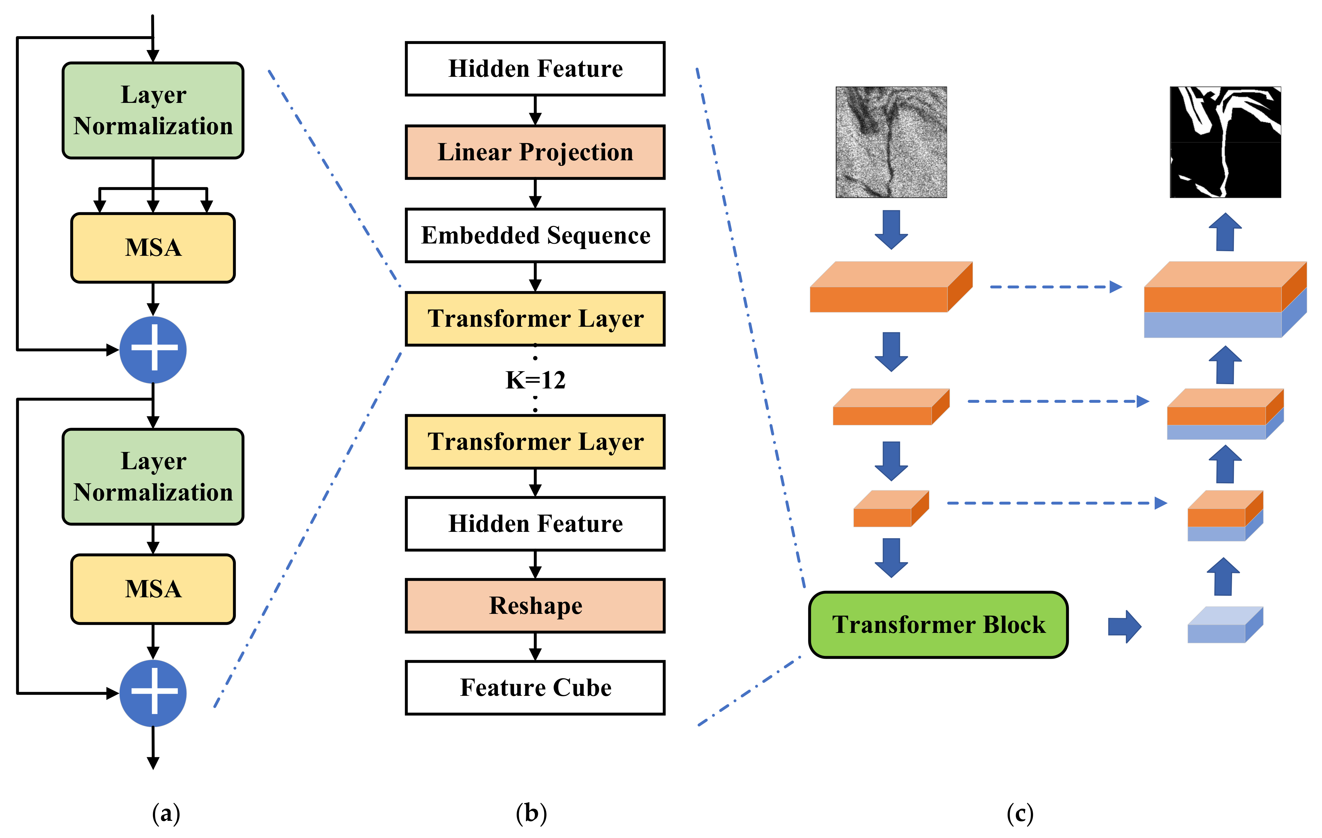
The architecture of the proposed oil spill detection model is shown as Figure 3.
The oil spill remote sensing image is the input, denoted by x H × W × C , where H × W is the image resolution and C is the number of channels. The goal is pixel-level classification, i.e., to generate a label map that corresponds to the input image on a pixel-by-pixel basis, which has a size of H × W , and each pixel point represents a category. The proposed oil spill detection model uses an encoder–decoder network structure. A hybrid model of a convolutional neural network (CNN) [43,44] and Transformer [45,46] is used as the encoder. The encoding process is carried out by first extracting the image features using the CNN, and the extracted results are then encoded by a Transformer block. The Transformer block is able to describe the interactions of different local regions in the image, so that the input sequence has global contextual information, in order to enhance the oil spill region with finer details by recovering local spatial information. The decoder upsamples the encoded features, and then, combines them with a high-resolution CNN feature map to achieve pixel-level pinpointing. The whole network structure can be considered as adding the Transformer block to the encoder part of the UNet semantic partition network, as shown in Figure 3c.

3.2. Transformer Block

The Transformer block contains a linear projection layer, 12 Transformer layers, and a reshape layer. The overall structure and computational flow of the Transformer block are shown in Figure 3b. The input x H × W × C is reshaped into a sequence of flattened 2D patches x p N × P 2 C , where P , P is the resolution of each image patch, and N = H W / P 2 is the resulting number of patches. To be able to use the Transformer properly, as in Equation (1), through a trainable linear projection, as shown in Figure 3b, the vector patches x p are mapped to a potentially D-dimensional embedding space [47].
z 0 = x p 1 E ; x p 2 E ; ; x p N E + E p o s ,   E P 2 C × D , E p o s N + 1 × D
where E is the patch embedding projection, and E p o s is the position embedding.
Each Transformer layer consists of a multi-head self-attentive module and a multilayer perception module, and the output of the kth deformer layer can be obtained using Equations (2) and (3). Figure 3a illustrates the structure of the Transformer layer.
z k = M S A L N z k 1 + z k 1
z k = M L P L N z k + z k
where L N · denotes the layer normalization operation, M S A denotes the multi-head self-attentive module, M L P denotes the multi-layer perception module, and z denotes the encoded image representation. In the self-attentive mechanism, each element in the input sequence interacts with other elements in the sequence to compute a contextual representation of each element. The multi-head self-attentive mechanism adds to this multiple independent attention heads, each with its own parameters, to allow the model to compute attention in different representation spaces. In each head, the input vectors are first divided into different dimensions; then, attention is computed in each subspace, and finally the representations generated by all the heads are stitched together to form the final contextual virtual representation. Our proposed method goes through the multi-head self-attentive mechanism to capture different aspects of information in the input sequence and process them in different representation spaces.

3.3. Loss Function

We use the sum of BCE loss and DICE loss as the loss function, as shown in Equation (4), where BCE stands for Binary Cross-Entropy and DICE stands for Sørensen–Dice coefficient. BCE loss is usually used in binary classification problems [48], as shown in Equation (5). DICE loss is defined as 1 minus the DICE similarity between the predicted and true labels [49], which is often used in tasks such as image segmentation and medical image processing to evaluate the similarity of the predicted segmentation results, as shown in Equation (6).
L l o s s = L B C E + L D I C E
L B C E = 1 N i = 1 N y i log y ^ i + 1 y i log 1 y ^ i
L D I C E = 1 2 i = 1 N y i y ^ i + 1 / i = 1 N y i + i = 1 N y ^ i + 1
where y i is the true label of the i th sample, y ^ i is the label predicted by the model of the i th sample, and N is the number of samples.
The two loss functions are combined to more comprehensively assess the performance of the model in classification and segmentation tasks. Specifically, the BCE loss function measures classification performance by comparing the differences between the binary classification results predicted by the model and the true labels, while the DICE loss function measures the degree of overlap between the segmentation results predicted by the model and the true segmentation results. By minimizing both the BCE and DICE loss functions, the model can be made to better balance the performance of classification and segmentation.

3.4. Experimental Environment and Control Model Selection

TensorFlow was chosen as the deep learning framework [50,51], and the proposed model was trained on a Nvidia V100 GPU. The optimizer used Adam [52] with an initial learning rate of 1 × 10⁻⁴. The performance of the proposed method is illustrated in comparison with common remote sensing semantic segmentation models such as UNet, SegNet, and DeepLabV3+, which are also trained using the same parameters and approach. The batch size was set to 4 [53], and each model was trained for 100 iterations on the entire training dataset. The oil spill detection model in Section 4 and Section 5 also used the experimental settings described above and will not be repeated subsequently. Also, to avoid redundancy, the experimental results and comparative analyses are presented in Section 6.2 and Section 6.3. Compared with UNet, DeepLabV3+, and SegNet, our proposed model has better performance, which also proves the feasibility of our research method.

4. Oil Spill Detection Model Based on TransUNet and FFDNet

In real situations, some remote sensing images may be affected by various factors, such as atmosphere, clouds, fog, sunlight irradiation, sensor noise, etc. These factors can lead to noise, distortion, and artifacts in the images. Therefore, in these cases, the denoising of remote sensing images can reduce the influence of these interfering factors on semantic segmentation, and thus, improve the accuracy of segmentation. Removing SAR coherent spots is a challenge because of SAR’s multiplicative noise property. In this section, we try to improve the FFDNet to denoise the remote sensing images first, and then, use the model proposed in Section 3 for oil spill detection.

4.1. FFDNet-Based SAR Image Denoising

FFDNet is a fast and flexible image noise reduction algorithm based on a deep convolutional neural network, non-local block filter, and fast Fourier transform to achieve efficient noise reduction [54]. FFDNet is capable of noise reduction for different types of image noise, including Gaussian noise, impulse noise, and mixed noise. It further improves the noise reduction effect by introducing residual learning to the CNN and employs a flexible training strategy, which makes the algorithm more general and applicable. The network architecture of FFDNet is shown in Figure 4, which mainly includes the downsampling part, the nonlinear mapping part, and the upsampling part. The core part is the nonlinear mapping part, which is shown in the middle part of Figure 4. It consists of 15 convolutional layers, and each layer performs three types of operation, namely convolution (Conv), rectified linear units (ReLU) [55], and batch normalization (BN) [56,57].
The type of noise that can be removed is controlled by the Noise Level Map. The original version of FFDNet was created to solve the additive noise denoising problem. In order to give FFDNet the ability to remove coherent speckle noise, we need to convert the coherent speckle noise into the form of additive fluctuations. The idea is to convert multiplicative fluctuations to additive fluctuations via logarithmic transformation of the original data, while transforming the coherent speckle noise model into a Fisher–Tippett distribution [58].
Assume that the original data are represented by Y , which consists of reflectance and the coherent spot component, i.e., Y = X × S , where X denotes reflectance and S denotes the coherent spot component. Upon performing logarithmic transformation of the original data, i.e., y = log Y ,
y = log X + log S
Using the properties of logarithmic transformation, multiplicative fluctuations can be transformed into additive fluctuations. According to the Goodmann model [59], the coherent speckle noise model can be expressed as a gamma distribution with the following probability density function:
p I Y | X = L L Y L 1 Γ L X L exp L Y X
where Γ is the gamma function, Y is the image intensity, X is the image reflectance, and L is the number of observations. Following the logarithmic transformation of Equation (7), Equation (8) can be transformed into the following:
p y y | x = L L Γ L e L y x exp L e y x
where x = log X , y = log Y , and p y y | x denotes the probability density function of y given x . According to the definition of Fisher–Tippett distribution [58], when L is sufficiently large, p y y | x can be approximated as having Fisher–Tippett distribution. After the transformation, the noise has a nonzero mean over the log-transformed data, thus demonstrating that the variance no longer depends on the expectation, i.e., the fluctuations change into the form of signal-independent additive fluctuations.

4.2. Denoising Effect

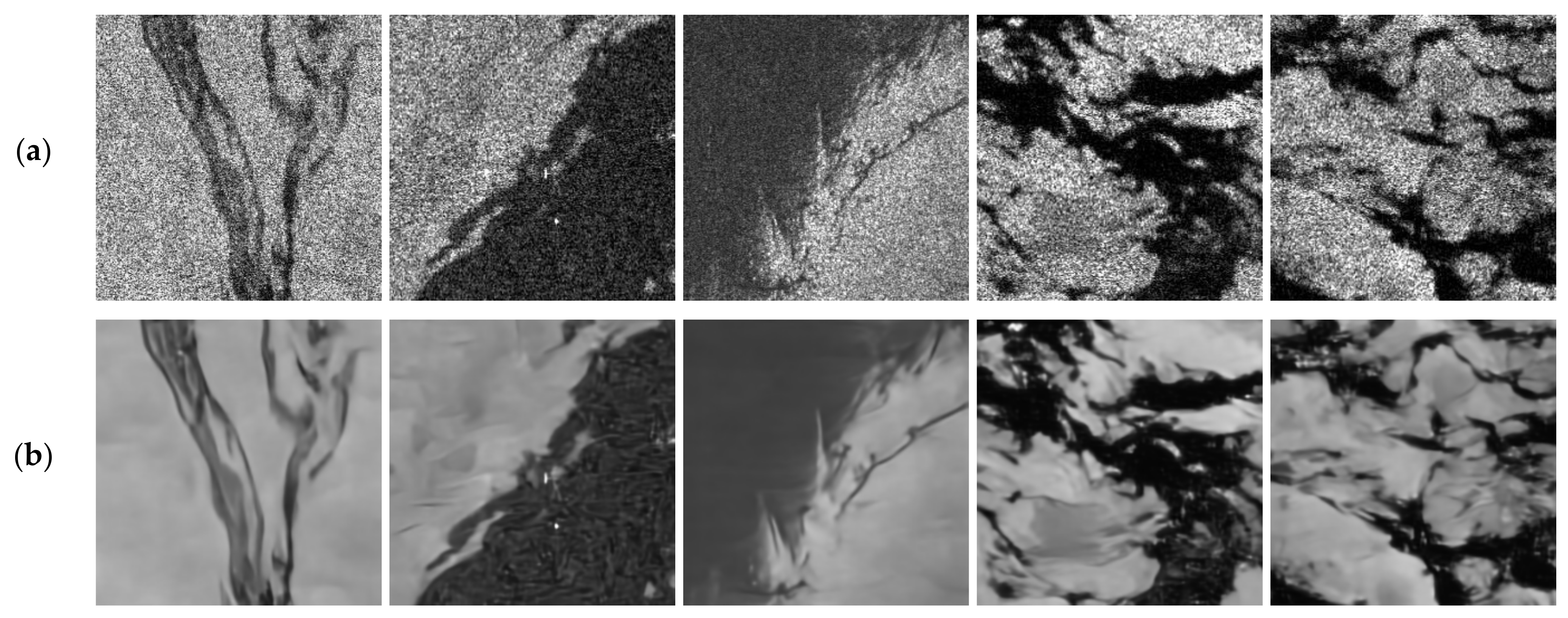
The remote sensing images in the dataset were processed using the above FFDNet-based denoising method, and improved results were obtained, as shown in Figure 5. Figure 5a shows the five original images from the Palsar dataset; the first one is the oil film detail image, the second and the third are the images of large oil spill zones with different edge conditions, and the fourth and the fifth are the images of oil spill areas with extremely irregular shapes due to the influence of seawater. Figure 5b shows the denoised images corresponding to Figure 5a, which demonstrates that image denoising is achieved with better preservation of the oil spill zone features. Also, based on the analysis of the dataset in Section 2, it can be found that the method proposed in this section has a suppression effect on the extensive noise.
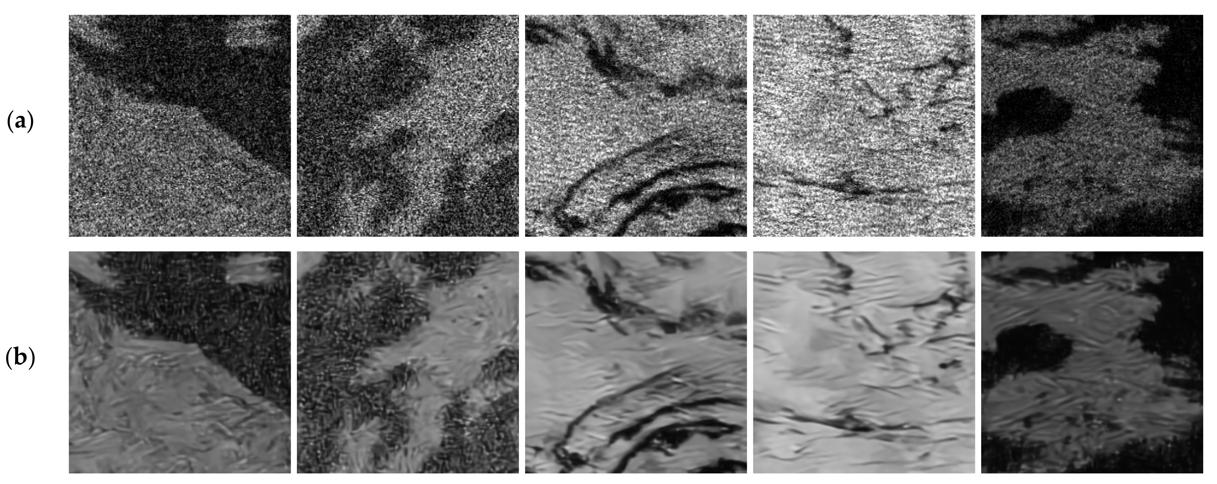
However, several examples of poor denoising exist, as shown in Figure 6. In Figure 6a, the first and second images have extremely contaminated noise, the third and fourth images are affected by moiré-like noise, and the fifth image suffers from complex noise and moiré-like noise at low luminance. Figure 6b shows the corresponding denoised images, and it can be seen that the denoising model does not remove the noise in the original image cleanly, especially the moiré-like noise, which is made sharper and more obvious after denoising. Normally, SAR images are not affected by light and darkness and do not have moiré-like noise with consistent noise levels, so the method described in this section should have very good results in processing conventional SAR images.

4.3. Oil Spill Detection Process

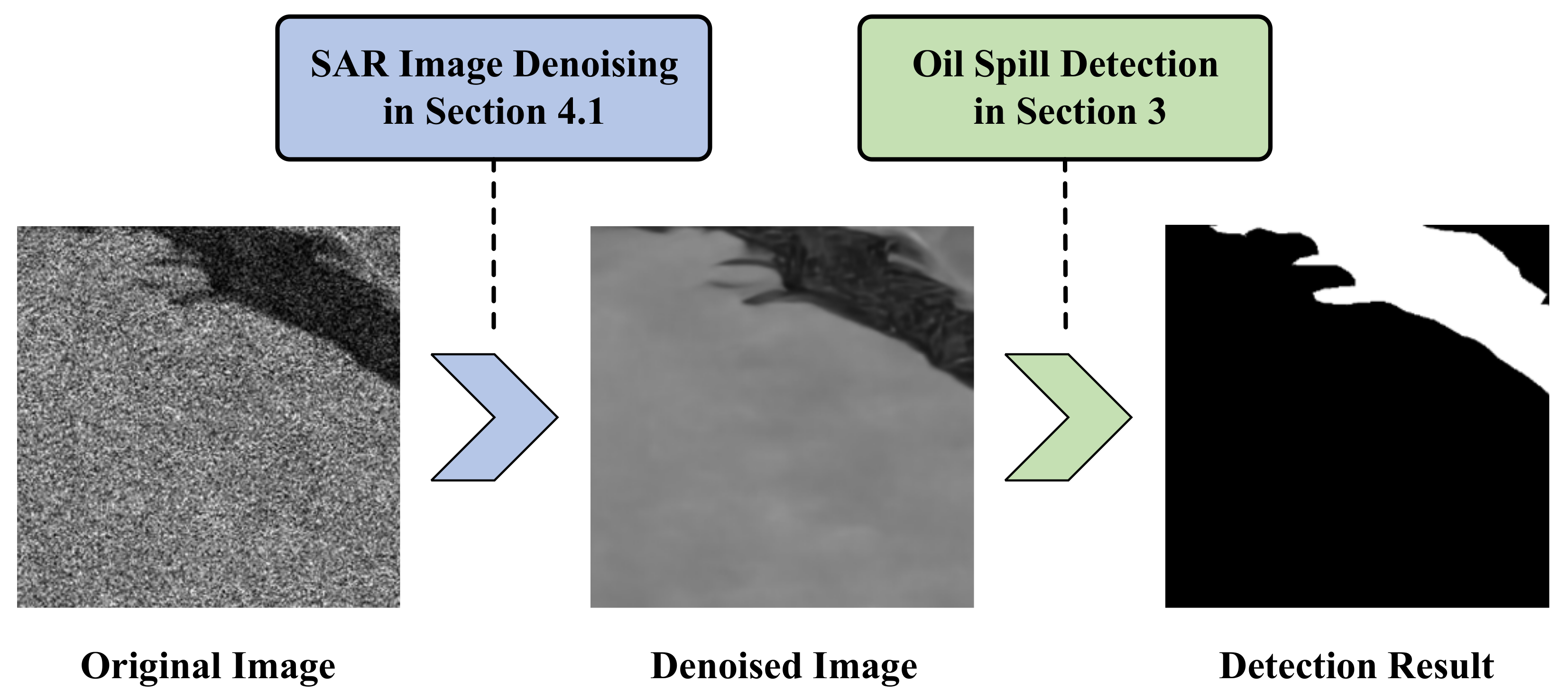
The training parameters of the detection model are basically the same as in Section 3 and are not repeated here. The oil spill detection process in this section is shown in Figure 7. Figure 7 shows the process from the original image to the denoised image to the final recognition result. Through the denoising process, the noise component in the original image can be reduced, thus improving the image quality and clarity. This helps to better understand and analyze the image features and contextual semantics, making the final detection result more accurate and reliable.

5. Model Ensemble

5.1. Algorithm Design

Model ensemble [60,61] is a method of combining multiple independently trained models to improve accuracy, stability, and generalization performance. This research problem is a binary classification problem where the identification of the oil (positive class) is more important than the identification of the sea (negative class); therefore, we use the OR operation to obtain the final result graphs by combining the positive-class results of multiple models, as shown in Equation (10).
F x = i = 1 n f i x
where f i x denotes the positive-class prediction of the i th model for input x , and denotes the logical OR operator. The output pixel point of F x is positive-class if there exists any model whose prediction is positive-class, otherwise it is negative-class.
The purpose of using the above approach is to enhance the overall model robustness by enhancing the identification of positive classes. Of course, there are certain problems with this approach, that is, it brings in many connected regions with small areas, i.e., fine noise is accumulated. Therefore, additional treatment is required for fine noise. In this experiment, we use an efficient method of removing the concatenated domain to achieve denoising. We perform a 4-neighborhood connected domain calculation on the final binary graph to obtain the set of all connected domains S . For the i th connected domain S i , it is processed according to Equation (11).
I x , y = 0 ,   x , y S i   if   S i S max
where I x , y denotes the pixel value of the position x , y in the binary image, x , y S i denotes that the position x , y belongs to the connected domain S i , S max denotes the connected domain containing the maximum number of pixels, and · denotes the number of pixels contained in the specified connected domain. This also means that when the number of pixels in a connected field is less than the threshold S max , the connected field is deleted. The threshold is set without the method of manually setting hyperparameters during conventional SAR image processing, with the aim of making the threshold-setting process adaptive. This proposed method achieves certain denoising effect regardless of the balance of positive- and negative-class data in the image.

5.2. System Implementation

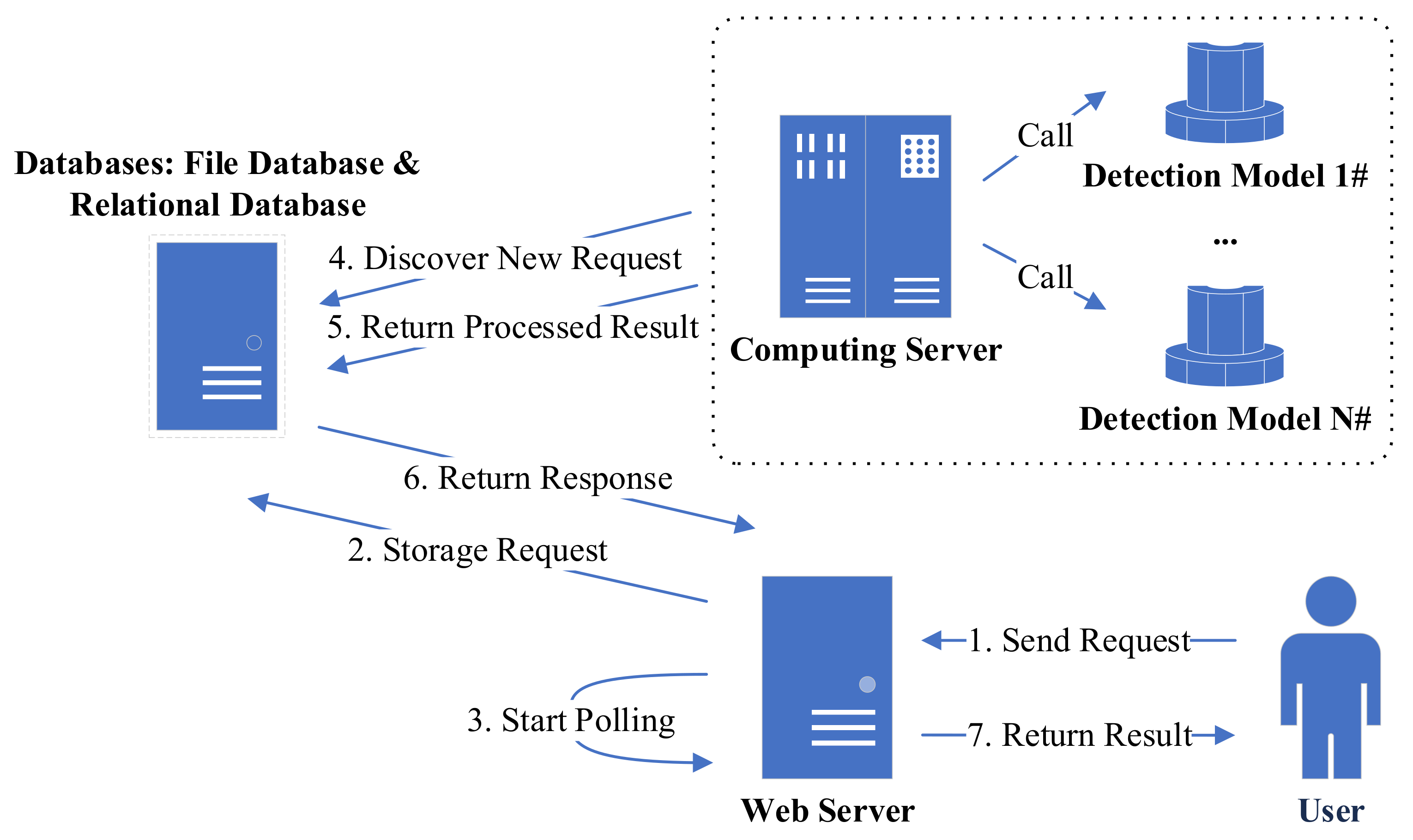
The aforementioned model integration approach allows for a looser form of architecture in the programming and supporting software development process, which also enhances the robustness and ease of scalability of the system to some extent. In this project, we completed the software system for oil spill detection through collaboration among models, and the information processing flow of this system is shown in Figure 8.
The user uploads the remote sensing image that needs to be processed, and the web server stores the remote sensing image on the file server and stores the user request in the relational database. The web employs AJAX (Asynchronous JavaScript and XML) technology [62], a frontend technique enabling asynchronous communication on web pages, to initiate polling until it finds the processing result of the request in the database before stopping. The computing server maintains millisecond polling of the relational database, and when a new request is found, it obtains the remote sensing image on the file server, calls the deep network model for analysis and calculation, returns the processed result to the file database after the calculation is completed, and updates the records in the relational database. The web server finds the updated feedback and invokes the processed result back to the user. When a new network model is added to the detection task, it can be directly deployed and completed to join the existing detection system, and only requires fine-tuning of the integration strategy in the computing server part.
The robustness of this architectural approach is mainly demonstrated by its ability to continue functioning even when any component in the system experiences an issue, except for database failures. Scalability is primarily manifested as the capability of adding or removing deep learning-based detection models as needed, which is a result of the simple integration method and loosely coupled architecture model. However, the system also possesses certain limitations, mainly related to the polling mechanism, which increases the workload on the database and leads to a less than fully real-time response to requests.

6. Experimental Results and Analysis

6.1. Evaluation Metrics

The images in the test set are predicted using the aforementioned models, and the segmentation masks of each image are connected and compared with the true value labels to establish the confusion matrix [63], from which the accuracy (A), precision (P), recall (R), F1-score (F1), and mean intersection over union (MIoU) are calculated to complete the evaluation of the detection model [64]. The oil spill area is defined as the positive class, while the non-oil spill area (i.e., the ocean) is defined as the negative class. The formulas for the above evaluation metrics are shown in Equations (12)–(16), respectively.
A = T P + T N / T P + T N + F P + F N
P = T P / T P + F P
R = T P / T P + F N
F 1 = 2 P R / P + R
M I o U = I o U P o s i t i v e + I o U N e g a t i v e 2 = T P / T P + F P + F N + T N / T N + F P + F N 2
where T P is the number of true positives, T N is the number of true negatives, F P is the number of false positives, and F N is the number of false negatives, and they are all elements of the confusion matrix.

6.2. Experimental Results for the Palsar Dataset

Experimental and quantitative analyses were conducted on the Palsar dataset according to the evaluation metrics designed, as described previously. For simplicity, we abbreviate the models in Section 3, Section 4 and Section 5 as M1, M2, and M3, respectively, i.e., M1 is the TransUNet-based Oil Spill Detection Model, M2 is the Oil Spill Detection Model Based on TransUNet and FFDNet, and M3 is the multi-model ensemble, which is used in the subsequent sections of this paper. Experimental validation was conducted, and the confusion matrices for each model were computed, as shown in Table 2. Based on these matrices and following the guidelines presented in Section 6.1, model evaluation was performed, and the results are presented in Table 3. The bold values in both tables represent the best performance in each evaluation dimension. The inclusion of detailed confusion matrices aims to provide readers with a better understanding of and means to verify the authenticity of the experimental results. Overall, M3 achieved the best performance with the best accuracy (93.58%), recall (97.28%), F1-score (96.18%), and the next best score in the MIoU metric (79.48%). In terms of MIoU metrics, the performance of M1, M2, and M3 is much higher than the other three models. Compared with the three selected benchmark remote sensing semantic segmentation models, the performance of M1 achieved an advantage in all evaluation metrics, which proves the effectiveness of this research method. M2 was created on the basis of M1, but its performance does not exceed that of M1, probably because the denoising model is for coherent speckle noise, and the data set contains complex noise other than coherent speckle noise. M2 has a greater advantage when it comes to semantic segmentation tasks for conventional SAR images. M3 is the model integration of M1 and M2, and obtains the best results not only in several evaluation dimensions but also in TP identification (as shown in Table 2), which matches the more important requirement of oil identification in this problem.

6.3. Experimental Results on the Sentinel Dataset

Experiments and quantitative analyses were performed on the Sentinel dataset using the same means as the experiments on the Palsar dataset. The confusion matrices for each model are shown in Table 4, and the experimental results are compared in Table 5. Similar to the experimental results of the Palsar dataset, good evaluation results were obtained for M1, M2, and M3. Among the total of six image segmentation models, M1 obtained the best in accuracy (93.41%) and MIoU (78.06%), and M3 was the best in accuracy (88.97%), recall (96.79%), and F1-score (91.97%). In terms of MIoU metrics, M1, M2, and M3 all outperformed the benchmark models.

6.4. Experimental Analysis

M1 improves global context-awareness by introducing Transformer, improves the model’s understanding and utilization of spatial information by introducing positional encoding, and has good robustness to transformations such as rotation, scaling, and cropping of the input image, thus achieving improved performance compared to the benchmark models. It is experimentally demonstrated that M1 uses a combination of Transformer and UNet, making it possible to better capture semantic information in images using the global attention mechanism of Transformer and the local feature extraction capability of UNet. M2 is an oil spill detection model built on the basis of being an excellent detection model for SAR images. In this dataset, although optical noise was artificially introduced in the image enhancement process, the largest source of noise is still coherent speckle noise, so M2 also shows good performance comparable to that of the benchmark models, and achieves a relative optimum in the precision rate metric. M3 integrates the calculated results of M1 and M2 using the OR operation, aiming to enhance the true positive values in the confusion matrix of detection results. The experimental results prove that the detection effect is further improved.
The experimental results for each model for the Palsar dataset are better than those for the Sentinel dataset. The sample sizes of the Palsar and Sentinel datasets are close, but there is a large difference in the ratio of positive- to negative-class samples, which is 83:17 in the Palsar dataset and 65:35 in the Sentinel dataset. This difference, and the potential difference in noise, causes a difference in the performance of the same model when dealing with different datasets. Taking M3 as an example, by analyzing its confusion matrix, it can be found that the percentage of FP is higher in the Sentinel dataset, accounting for 8.93% of the total pixel points, much higher than the value of 4.16% obtained when dealing with the Palsar dataset. The higher percentage of FP is the root cause of the performance difference, and the reasons for it may be the noise level and the quality of the gt_images.

6.5. Training and Inference Performance

Our experiments show the performance advantage of our proposed models, which is caused by the larger parameter size and more complex network hierarchy. The training time for M1 and M2 is much higher than UNet, SegNet, and DeepLabV3+ (roughly 3–4 times higher). Although more training time is needed, it is still within the allowable range for now. M3 is essentially a model integration algorithm that does not require training, and the integration time can be largely ignored. The specific training time of each model is shown in Table 6.
Starting from the model’s initial loading time and single-image prediction time, we analyzed the inference performance of each model, and the results are shown in Table 7. The proposed methods in this paper, due to their more complex network structures and higher parameter counts, have loading times that are 2.5 to 6.5 times longer than traditional models, and memory usage is also proportional to this factor. However, since the model only needs to be loaded once, the associated overhead is acceptable. In terms of single-image prediction time, our proposed method takes 2.2 to 2.8 times longer than traditional models, clearly showing that the model sacrifices time for improved performance through more complex computations. The prediction time of M3 in serial mode is the sum of the prediction times of all models, while in parallel mode, the minimum prediction time is determined by the slowest model among all the models. This means that the prediction time of M3 lies between these two extreme values. In practical applications, the integration method of M3 is configured based on the available schedulable resources.

6.6. Supplementary Explanation

References [26,35] are the original papers proposing the SOS dataset, but there are possible errors in the experimental results therein. According to Equation (15), the value of F1-score is the harmonic mean of precision (P) and recall (R), and its value should be between P and R. The following three experimental results in the two aforementioned original manuscripts clearly violate this rule:
  • In the experimental results of the Sentinel sub-dataset presented in reference [26], the UNET-based approach achieved an F1 of 86.10, R of 81.22, and P of 85.61.
  • In the experimental results of the Sentinel sub-dataset presented in reference [26], the DLinkNet-based approach achieved an F1 of 87.08, R of 85.22, and P of 85.22.
  • In the experimental results of the Palsar sub-dataset presented in reference [35], the UNET-based approach obtained an F1 of 96.36, R of 95.4, and P of 95.35.
In the three examples above, the values of the F1 are greater than both P and R, which defies common sense, and in the second example, P and R are exactly equal, which is also extremely rare. In addition to the obvious errors mentioned above, there are a number of other experimental results in the two papers where the F1 is clearly biased in favor of either P or R, which is also worth discussing and questioning. This experimental result is not worth faking, and the probability is that there is an error in the model evaluation algorithm. In summary, the experimental results in references [26,35] have more contradictions, and thus, cannot be used as a reference or benchmark for research in this field. The original intention of this paper is to provide a more reliable benchmark for related research. To facilitate the verification of the authenticity of the experimental data, Table 2 and Table 4 in this manuscript display the raw confusion matrix data. Subsequent research can use the experimental results in this article as a reference.

7. Discussion and Conclusions

The SOS dataset is a very creative dataset in oil spill detection, containing the Gulf of Mexico oil spill area and the Persian Gulf oil spill area, acquired from ALOS and Sentinel-1A satellites, respectively, and is a pixel-level dataset of oil spills and non-oil spills. The artificial inclusion of diverse noise in this dataset makes the detection task much more difficult. This dataset provides research ideas and necessary datasets for studies related to marine oil spill detection from low-quality SAR remote sensing images. The label quality of this dataset currently has some problems, and we will further refine and improve it. The source code and the improved SOS dataset will be available at https://github.com/dongxr2/MOSD_LSAR (accessed on 27 July 2023). In the future, we will also attempt to utilize model compression techniques [65,66] to reduce resource consumption in practical applications, promote the engineering application of achievements, and incorporate more datasets and detection algorithms to improve this research direction.
In order to solve the problem of marine oil spill detection with low-quality SAR remote sensing images, we propose a TransUNet-based oil spill detection model in this paper, which combines Transformer and UNet to better capture the semantic information in images by using the global attention mechanism of Transformer and the local feature extraction capability of UNet. We modified FFDNet to have the ability to denoise SAR images and combined the denoising model with the TransUNet-based model to become an oil spill detection model capable of targeting those SAR images with no artificially added noise interference. The model was developed to match realistic applications of SAR image-based oil spill detection, but it is also tolerant to optical noise and has slightly higher performance than common remote sensing semantic segmentation models such as UNet and SegNet.
In order to match the need for positive classes to be much more important than negative classes, we propose a model integration approach that integrates the two aforementioned models to collaborate on the detection task. At the same time, we propose a simple and easy way to deal with the subtle noise introduced during the integration process, and give a feasible, highly robust, and easily scalable system design method for system implementation.
In summary, this paper gives a multi-faceted solution for oil spill detection based on the SOS dataset, and the three proposed models all have better detection performance compared to conventional semantic segmentation models. For the experimental part, we give the performance of each model and its database. The experimental results in references [26,35] have more contradictions and cannot serve as a reference or comparison for related studies. The experimental methods and performance details in this paper can provide a reference for related studies. The Transformer block, coherent spot denoising algorithm, multi-model ensemble, and other methods introduced in this paper can effectively improve the performance of image segmentation, and provide new ideas and directions for research related to marine oil spill detection based on deep learning, and the proposed research results of remote sensing semantic segmentation can be combined with related theories and technologies to explore more effective solutions for marine oil spill detection.

Author Contributions

Conceptualization, X.D., J.L., Y.J. and S.M.; methodology, X.D. and B.L.; software, X.D., B.L. and Y.J.; validation, X.D., J.L. and S.M.; formal analysis, X.D.; investigation, X.D.; resources, X.D., Y.J. and S.M.; data curation, X.D. and J.L.; writing—original draft preparation, X.D.; writing—review and editing, X.D., J.L. and B.L.; visualization, X.D.; supervision, X.D.; project administration, X.D.; funding acquisition, X.D., J.L., Y.J. and S.M. All authors have read and agreed to the published version of the manuscript.

Funding

This research was funded by a specially funded open project of the Key Laboratory of Electric Wave Environmental Characteristics and Modeling Technology (Grant No. 202102009), and the Dongying Science Development Fund (Grant No. DJ2022010).

Institutional Review Board Statement

Not applicable.

Informed Consent Statement

Not applicable.

Data Availability Statement

An introduction to the dataset studied in this paper can be found at: https://grzy.cug.edu.cn/zhuqiqi. The dataset can be downloaded from: http://cugurs5477.mikecrm.com/5tk5gyO (accessed on 27 July 2023).

Acknowledgments

We acknowledge Qiqi Zhu and others for making and sharing the SOS dataset. We acknowledge the Dongying Key Laboratory of Intelligent Information Processing for the computing power support provided for this research. We acknowledge the Dongying Artificial Intelligence and Data Mining Laboratory for providing hardware equipment support. We acknowledge Kai Shang’s for sharing his experience and bringing inspiration to this research.

Conflicts of Interest

The authors declare no conflict of interest.

References

  1. Rayner, R.; Jolly, C.; Gouldman, C. Ocean Observing and the Blue Economy. Front. Mar. Sci. 2019, 6, 330. [Google Scholar] [CrossRef]
  2. Jolly, C. The Ocean Economy in 2030. In Proceedings of the the Workshop on Maritime Cluster and Global Challenges 50th Anniversary of the WP6, Paris, France, 1 December 2016; Volume 1. [Google Scholar]
  3. Virdin, J.; Vegh, T.; Jouffray, J.-B.; Blasiak, R.; Mason, S.; Österblom, H.; Vermeer, D.; Wachtmeister, H.; Werner, N. The Ocean 100: Transnational Corporations in the Ocean Economy. Sci. Adv. 2021, 7, eabc8041. [Google Scholar] [CrossRef]
  4. Prince, R.C. A Half Century of Oil Spill Dispersant Development, Deployment and Lingering Controversy. Int. Biodeterior. Biodegrad. 2023, 176, 105510. [Google Scholar] [CrossRef]
  5. He, F.; Ma, J.; Lai, Q.; Shui, J.; Li, W. Environmental Impact Assessment of a Wharf Oil Spill Emergency on a River Water Source. Water 2023, 15, 346. [Google Scholar] [CrossRef]
  6. Miloslavich, P.; Seeyave, S.; Muller-Karger, F.; Bax, N.; Ali, E.; Delgado, C.; Evers-King, H.; Loveday, B.; Lutz, V.; Newton, J.; et al. Challenges for Global Ocean Observation: The Need for Increased Human Capacity. J. Oper. Oceanogr. 2019, 12, S137–S156. [Google Scholar] [CrossRef] [Green Version]
  7. Weller, R.A.; Baker, D.J.; Glackin, M.M.; Roberts, S.J.; Schmitt, R.W.; Twigg, E.S.; Vimont, D.J. The Challenge of Sustaining Ocean Observations. Front. Mar. Sci. 2019, 6, 105. [Google Scholar]
  8. Li, P.; Cai, Q.; Lin, W.; Chen, B.; Zhang, B. Offshore Oil Spill Response Practices and Emerging Challenges. Mar. Pollut. Bull. 2016, 110, 6–27. [Google Scholar] [CrossRef]
  9. Pandey, S.K.; Kim, K.-H.; Yim, U.-H.; Jung, M.-C.; Kang, C.-H. Airborne Mercury Pollution from a Large Oil Spill Accident on the West Coast of Korea. J. Hazard. Mater. 2009, 164, 380–384. [Google Scholar] [CrossRef] [PubMed]
  10. Storrie, J. Montara Wellhead Platform Oil Spill—A Remote Area Response. Int. Oil Spill Conf. Proc. 2023, 2011, 159. [Google Scholar] [CrossRef]
  11. Carvalho, G.D.A.; Minnett, P.J.; De Miranda, F.P.; Landau, L.; Paes, E.T. Exploratory Data Analysis of Synthetic Aperture Radar (SAR) Measurements to Distinguish the Sea Surface Expressions of Naturally-Occurring Oil Seeps from Human-Related Oil Spills in Campeche Bay (Gulf of Mexico). ISPRS Int. J. Geo-Inf. 2017, 6, 379. [Google Scholar] [CrossRef] [Green Version]
  12. Xu, H.-L.; Chen, J.-N.; Wang, S.-D.; Liu, Y. Oil Spill Forecast Model Based on Uncertainty Analysis: A Case Study of Dalian Oil Spill. Ocean. Eng. 2012, 54, 206–212. [Google Scholar] [CrossRef]
  13. Liu, X.; Guo, J.; Guo, M.; Hu, X.; Tang, C.; Wang, C.; Xing, Q. Modelling of Oil Spill Trajectory for 2011 Penglai 19-3 Coastal Drilling Field, China. Appl. Math. Model. 2015, 39, 5331–5340. [Google Scholar] [CrossRef]
  14. Li, Y.; Yu, H.; Wang, Z.; Li, Y.; Pan, Q.; Meng, S.; Yang, Y.; Lu, W.; Guo, K. The Forecasting and Analysis of Oil Spill Drift Trajectory during the Sanchi Collision Accident, East China Sea. Ocean. Eng. 2019, 187, 106231. [Google Scholar] [CrossRef]
  15. Li, K.; Yu, H.; Xu, Y.; Luo, X. Scheduling Optimization of Offshore Oil Spill Cleaning Materials Considering Multiple Accident Sites and Multiple Oil Types. Sustainability 2022, 14, 10047. [Google Scholar] [CrossRef]
  16. Li, K.; Ouyang, J.; Yu, H.; Xu, Y.; Xu, J. Overview of Research on Monitoring of Marine Oil Spill. IOP Conf. Ser. Earth Environ. Sci. 2021, 787, 012078. [Google Scholar] [CrossRef]
  17. Li, K.; Yu, H.; Yan, J.; Liao, J. Analysis of Offshore Oil Spill Pollution Treatment Technology. IOP Conf. Ser. Earth Environ. Sci. 2020, 510, 042011. [Google Scholar] [CrossRef]
  18. Brekke, C.; Solberg, A.H.S. Oil Spill Detection by Satellite Remote Sensing. Remote Sens. Environ. 2005, 95, 1–13. [Google Scholar] [CrossRef]
  19. Hass, F.S.; Jokar Arsanjani, J. Deep Learning for Detecting and Classifying Ocean Objects: Application of YoloV3 for Iceberg–Ship Discrimination. ISPRS Int. J. Geo-Inf. 2020, 9, 758. [Google Scholar] [CrossRef]
  20. Pinho, J.L.S.; Antunes Do Carmo, J.S.; Vieira, J.M.P. Numerical Modelling of Oil Spills in Coastal Zones. A Case Study. WIT Trans. Ecol. Environ. 2002, 59, 35–45. [Google Scholar]
  21. Inan, A. Modeling of Oil Pollution in Derince Harbor. J. Coast. Res. 2011, SI 64, 894–898. [Google Scholar]
  22. Cho, Y.-S.; Kim, T.-K.; Jeong, W.; Ha, T. Numerical Simulation of Oil Spill in Ocean. J. Appl. Math. 2012, 2012, e681585. [Google Scholar] [CrossRef] [Green Version]
  23. Iouzzi, N.; Ben Meftah, M.; Haffane, M.; Mouakkir, L.; Chagdali, M.; Mossa, M. Modeling of the Fate and Behaviors of an Oil Spill in the Azemmour River Estuary in Morocco. Water 2023, 15, 1776. [Google Scholar] [CrossRef]
  24. Keramea, P.; Spanoudaki, K.; Zodiatis, G.; Gikas, G.; Sylaios, G. Oil Spill Modeling: A Critical Review on Current Trends, Perspectives, and Challenges. J. Mar. Sci. Eng. 2021, 9, 181. [Google Scholar] [CrossRef]
  25. Khan, M.; El Saddik, A.; Alotaibi, F.S.; Pham, N.T. AAD-Net: Advanced End-to-End Signal Processing System for Human Emotion Detection & Recognition Using Attention-Based Deep Echo State Network. Knowl.-Based Syst. 2023, 270, 110525. [Google Scholar] [CrossRef]
  26. Zhu, Q.; Zhang, Y.; Li, Z.; Yan, X.; Guan, Q.; Zhong, Y.; Zhang, L.; Li, D. Oil Spill Contextual and Boundary-Supervised Detection Network Based on Marine SAR Images. IEEE Trans. Geosci. Remote Sens. 2022, 60, 1–10. [Google Scholar] [CrossRef]
  27. Prajapati, K.; Ramakrishnan, R.; Bhavsar, M.; Mahajan, A.; Narmawala, Z.; Bhavsar, A.; Raboaca, M.S.; Tanwar, S. Log Transformed Coherency Matrix for Differentiating Scattering Behaviour of Oil Spill Emulsions Using SAR Images. Mathematics 2022, 10, 1697. [Google Scholar] [CrossRef]
  28. Wang, D.; Wan, J.; Liu, S.; Chen, Y.; Yasir, M.; Xu, M.; Ren, P. BO-DRNet: An Improved Deep Learning Model for Oil Spill Detection by Polarimetric Features from SAR Images. Remote Sens. 2022, 14, 264. [Google Scholar] [CrossRef]
  29. Ma, X.; Xu, J.; Wu, P.; Kong, P. Oil Spill Detection Based on Deep Convolutional Neural Networks Using Polarimetric Scattering Information From Sentinel-1 SAR Images. IEEE Trans. Geosci. Remote Sens. 2022, 60, 1–13. [Google Scholar] [CrossRef]
  30. Temitope Yekeen, S.; Balogun, A.; Wan Yusof, K.B. A Novel Deep Learning Instance Segmentation Model for Automated Marine Oil Spill Detection. ISPRS J. Photogramm. Remote Sens. 2020, 167, 190–200. [Google Scholar] [CrossRef]
  31. Bianchi, F.M.; Espeseth, M.M.; Borch, N. Large-Scale Detection and Categorization of Oil Spills from SAR Images with Deep Learning. Remote Sens. 2020, 12, 2260. [Google Scholar] [CrossRef]
  32. Ronneberger, O.; Fischer, P.; Brox, T. U-Net: Convolutional Networks for Biomedical Image Segmentation. In Proceedings of the Medical Image Computing and Computer-Assisted Intervention—MICCAI 2015, Munich, Germany, 5–9 October 2015; Springer International Publishing: Cham, Switzerland, 2015; pp. 234–241. [Google Scholar]
  33. Badrinarayanan, V.; Kendall, A.; Cipolla, R. SegNet: A Deep Convolutional Encoder-Decoder Architecture for Image Segmentation. IEEE Trans. Pattern Anal. Mach. Intell. 2017, 39, 2481–2495. [Google Scholar] [CrossRef]
  34. Chen, L.-C.; Papandreou, G.; Schroff, F.; Adam, H. Rethinking Atrous Convolution for Semantic Image Segmentation. arXiv 2017. [Google Scholar] [CrossRef]
  35. Zhang, Y.; Zhu, Q.; Guan, Q. Oil Spill Detection Based on CBD-Net Using Marine SAR Image. In Proceedings of the 2021 IEEE International Geoscience and Remote Sensing Symposium IGARSS, Brussels, Belgium, 11–16 July 2021; pp. 3495–3498. [Google Scholar]
  36. SkyTruth Gulf Oil Spill Covers 817 Square Miles. Available online: https://skytruth.org/2010/04/gulf-oil-spill-covers-817-square-miles/ (accessed on 28 July 2023).
  37. SkyTruth Satellite Imagery Reveals Scope of Last Week’s Oil Spill in Kuwait. Available online: https://skytruth.org/2017/08/satellite-imagery-reveals-scope-of-last-weeks-massive-oil-spill-in-kuwait/ (accessed on 28 July 2023).
  38. Erkan, U.; Thanh, D.N.H.; Hieu, L.M.; Engínoğlu, S. An Iterative Mean Filter for Image Denoising. IEEE Access 2019, 7, 167847–167859. [Google Scholar] [CrossRef]
  39. De Oliveira, M.E.; de Oliveira, G.N.; de Souza, J.C.; dos Santos, P.A.M. Photorefractive Moiré-like Patterns for the Multifringe Projection Method in Fourier Transform Profilometry. Appl. Opt. 2016, 55, 1048–1053. [Google Scholar] [CrossRef] [PubMed]
  40. Luo, P.; Zhang, M.; Ghassemlooy, Z.; Le Minh, H.; Tsai, H.-M.; Tang, X.; Png, L.C.; Han, D. Experimental Demonstration of RGB LED-Based Optical Camera Communications. IEEE Photonics J. 2015, 7, 1–12. [Google Scholar] [CrossRef]
  41. Vaswani, A.; Shazeer, N.; Parmar, N.; Uszkoreit, J.; Jones, L.; Gomez, A.N.; Kaiser, Ł.; Polosukhin, I. Attention Is All You Need. In Proceedings of the the 31st International Conference on Neural Information Processing Systems, Long Beach, CA, USA, 4–9 December 2017; Curran Associates Inc.: Red Hook, NY, USA, 2017; pp. 6000–6010. [Google Scholar]
  42. Chen, J.; Lu, Y.; Yu, Q.; Luo, X.; Adeli, E.; Wang, Y.; Lu, L.; Yuille, A.L.; Zhou, Y. TransUNet: Transformers Make Strong Encoders for Medical Image Segmentation. arXiv 2021. [Google Scholar] [CrossRef]
  43. Ajit, A.; Acharya, K.; Samanta, A. A Review of Convolutional Neural Networks. In Proceedings of the 2020 International Conference on Emerging Trends in Information Technology and Engineering (ic-ETITE), Vellore, India, 24–25 February 2020; pp. 1–5. [Google Scholar]
  44. Liu, B.; Li, Y.; Li, G.; Liu, A. A Spectral Feature Based Convolutional Neural Network for Classification of Sea Surface Oil Spill. ISPRS Int. J. Geo-Inf. 2019, 8, 160. [Google Scholar] [CrossRef] [Green Version]
  45. Parmar, N.; Vaswani, A.; Uszkoreit, J.; Kaiser, L.; Shazeer, N.; Ku, A.; Tran, D. Image Transformer. In Proceedings of the the 35th International Conference on Machine Learning, Stockholm, Sweden, 10–15 July 2018; pp. 4055–4064. [Google Scholar]
  46. Liu, Z.; Lin, Y.; Cao, Y.; Hu, H.; Wei, Y.; Zhang, Z.; Lin, S.; Guo, B. Swin Transformer: Hierarchical Vision Transformer Using Shifted Windows. In Proceedings of the the IEEE/CVF International Conference on Computer Vision, Montreal, BC, Canada, 11–17 October 2021; pp. 10012–10022. [Google Scholar]
  47. Dosovitskiy, A.; Beyer, L.; Kolesnikov, A.; Weissenborn, D.; Zhai, X.; Unterthiner, T.; Dehghani, M.; Minderer, M.; Heigold, G.; Gelly, S.; et al. An Image Is Worth 16 × 16 Words: Transformers for Image Recognition at Scale. arXiv 2021. [Google Scholar] [CrossRef]
  48. Ruby, U.; Yendapalli, V. Binary Cross Entropy with Deep Learning Technique for Image Classification. Int. J. Adv. Trends Comput. Sci. Eng. 2020, 9, 5393–5397. [Google Scholar] [CrossRef]
  49. Li, X.; Sun, X.; Meng, Y.; Liang, J.; Wu, F.; Li, J. Dice Loss for Data-Imbalanced NLP Tasks. arXiv 2020. [Google Scholar] [CrossRef]
  50. Abadi, M. TensorFlow: Learning Functions at Scale. In Proceedings of the the 21st ACM SIGPLAN International Conference on Functional Programming, Nara, Japan, 18–24 September 2016; Association for Computing Machinery: New York, NY, USA, 2016; p. 1. [Google Scholar]
  51. Pang, B.; Nijkamp, E.; Wu, Y.N. Deep Learning With TensorFlow: A Review. J. Educ. Behav. Stat. 2020, 45, 227–248. [Google Scholar] [CrossRef]
  52. Kingma, D.P.; Ba, J. Adam: A Method for Stochastic Optimization. arXiv 2017. [Google Scholar] [CrossRef]
  53. He, F.; Liu, T.; Tao, D. Control Batch Size and Learning Rate to Generalize Well: Theoretical and Empirical Evidence. In Proceedings of the Advances in Neural Information Processing Systems; Curran Associates, Inc.: Red Hook, NY, USA, 2019; Volume 32. [Google Scholar]
  54. Zhang, K.; Zuo, W.; Zhang, L. FFDNet: Toward a Fast and Flexible Solution for CNN-Based Image Denoising. IEEE Trans. Image Process. 2018, 27, 4608–4622. [Google Scholar] [CrossRef] [PubMed] [Green Version]
  55. Agarap, A.F. Deep Learning Using Rectified Linear Units (ReLU). arXiv 2019. [Google Scholar] [CrossRef]
  56. Bjorck, N.; Gomes, C.P.; Selman, B.; Weinberger, K.Q. Understanding Batch Normalization. In Proceedings of the Advances in Neural Information Processing Systems; Curran Associates, Inc.: Red Hook, NY, USA, 2018; Volume 31. [Google Scholar]
  57. Santurkar, S.; Tsipras, D.; Ilyas, A.; Madry, A. How Does Batch Normalization Help Optimization? In Proceedings of the Advances in Neural Information Processing Systems; Curran Associates, Inc.: Red Hook, NY, USA, 2018; Volume 31. [Google Scholar]
  58. Basrak, B. Fisher-Tippett Theorem. In International Encyclopedia of Statistical Science; Lovric, M., Ed.; Springer: Berlin/Heidelberg, Germany, 2011; pp. 525–526. ISBN 978-3-642-04898-2. [Google Scholar]
  59. Goodman, J.W. Some Effects of Target-Induced Scintillation on Optical Radar Performance. Proc. IEEE 1965, 53, 1688–1700. [Google Scholar] [CrossRef]
  60. Kurutach, T.; Clavera, I.; Duan, Y.; Tamar, A.; Abbeel, P. Model-Ensemble Trust-Region Policy Optimization. arXiv 2018. [Google Scholar] [CrossRef]
  61. Xiao, Y.; Wu, J.; Lin, Z.; Zhao, X. A Deep Learning-Based Multi-Model Ensemble Method for Cancer Prediction. Comput. Methods Programs Biomed. 2018, 153, 1–9. [Google Scholar] [CrossRef]
  62. Garrett, J.J. Ajax: A New Approach to Web Applications. Available online: https://courses.cs.washington.edu/courses/cse490h/07sp/readings/ajax_adaptive_path.pdf (accessed on 27 July 2023).
  63. Caelen, O. A Bayesian interpretation of the confusion matrix. Ann. Math. Artif. Intell. 2017, 81, 429–450. [Google Scholar] [CrossRef]
  64. Wang, Z.; Wang, E.; Zhu, Y. Image Segmentation Evaluation: A Survey of Methods. Artif. Intell. Rev. 2020, 53, 5637–5674. [Google Scholar] [CrossRef]
  65. Yang, G.; Lei, J.; Xie, W.; Fang, Z.; Li, Y.; Wang, J.; Zhang, X. Algorithm/Hardware Codesign for Real-Time On-Satellite CNN-Based Ship Detection in SAR Imagery. IEEE Trans. Geosci. Remote Sens. 2022, 60, 1–18. [Google Scholar] [CrossRef]
  66. Diana, L.; Xu, J.; Fanucci, L. Oil Spill Identification from SAR Images for Low Power Embedded Systems Using CNN. Remote Sens. 2021, 13, 3606. [Google Scholar] [CrossRef]
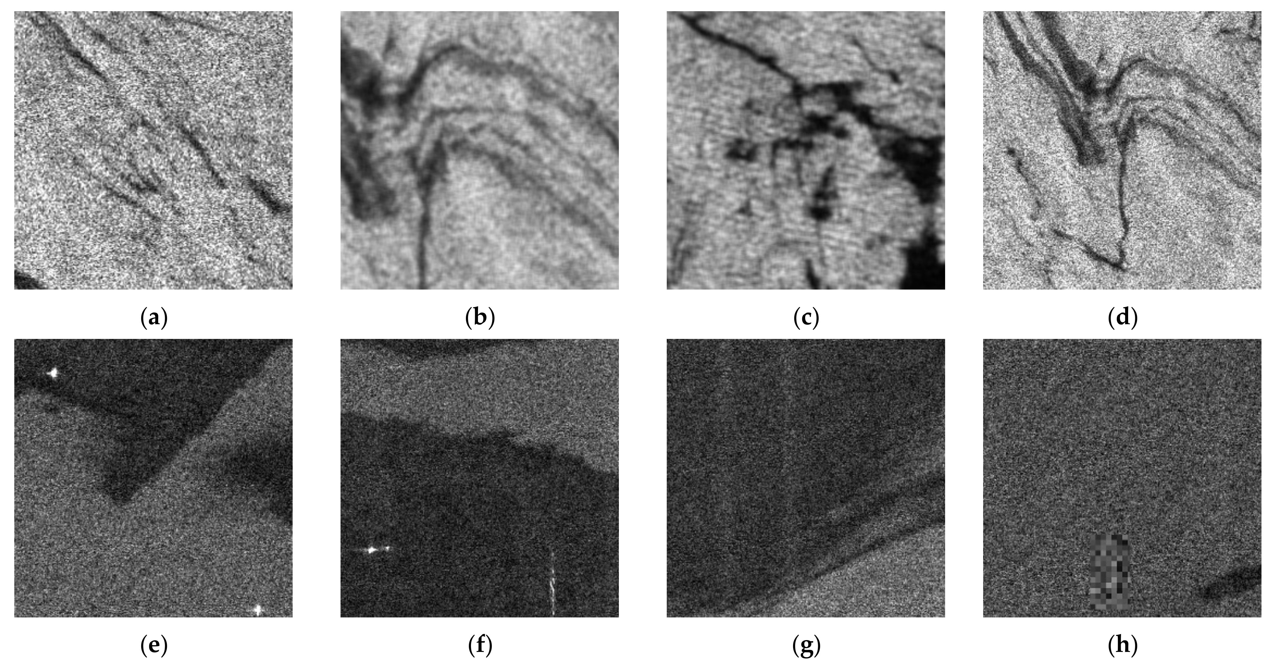
Figure 1. Eight training images affected by different typical artificial noise, including (a) 10,777_sat.jpg, (b) 11,019_sat.jpg, (c) 11,253_sat.jpg, (d) 12,037_sat.jpg, (e) 33,165_sat.jpg, (f) 33,261_sat.jpg, (g) 33,277_sat.jpg, (h) 33,291_sat.jpg in the training folder of the Palsar sub-dataset.
Jmse 11 01552 g001
Figure 2. Examples of labels with quality issues in the SOS dataset: (a) 33,282_mask.png; (b) local enlargement of 33,282_mask.png; (c) 33,259_mask.png; (d) local enlargement of 33,259_mask.png.
Jmse 11 01552 g002
Figure 3. The oil spill detection model: (a) the structure of the Transformer layer; (b) the overall structure and computational flow of the Transformer block; (c) the architecture of the proposed TransUNet-based oil spill detection model (adapted from [42]).
Jmse 11 01552 g003
Figure 4. The network architecture of FFDNet.
Jmse 11 01552 g004
Figure 5. Examples of effective denoising: (a) original images from the Palsar dataset; (b) denoised images.
Jmse 11 01552 g005
Figure 6. Examples of ineffective denoising: (a) original images from the Palsar dataset; (b) denoised images.
Jmse 11 01552 g006
Figure 7. The oil spill detection process.
Jmse 11 01552 g007
Figure 8. The information processing flow.
Jmse 11 01552 g008
Table 1. The composition of the SOS dataset.
Sub-DatasetImagesCapture DateLatitudeLongitude
Palsar datasetALPSRP23020056021 May 201028.734°−90.707°
ALPSRP23122054028 May 201027.739°−87.821°
ALPSRP23122056028 May 201028.728°−88.026°
ALPSRP23122058028 May 201029.723°−88.229°
ALPSRP2329705709 June 201029.224°−87.056°
ALPSRP2329705809 June 201029.721°−87.155°
ALPSRS2330430509 June 201028.389°−88.302°
ALPSRP23545056026 June 201028.728°−87.488°
ALPSRP23793055013 July 201028.233°−87.926°
ALPSRP23793056013 July 201028.728°−88.024°
ALPSRP23866050018 July 201025.758°−89.029°
ALPSRP23866055018 July 201028.237°−89.535°
ALPSRS23975310025 July 201025.719°−88.871°
ALPSRP2418705209 August 201026.749°−91.371°
Sentinel datasetIW_GRDH_1SDV_017782_01DCBB_DE285 August 201727.311°50.597°
IW_GRDH_1SDV_017848_01DEC1_EC329 August 201728.495°48.995°
IW_GRDH_1SDV_017848_01DEC1_C09A9 August 201729.002°48.660°
IW_GRDH_1SDV_017855_01DEF7_F48C10 August 201729.439°47.535°
IW_GRDH_1SDV_017884_01DFD8_8F9312 August 201727.014°52.812°
IW_GRDH_1SDV_017884_01DFD8_6CAE12 August 201725.505°52.485°
IW_GRDH_1SDV_017921_01EOED DB3914 August 201728.706°46.893°
Table 2. Confusion matrices for each model on the Palsar dataset.
ModelTPFNFPTN
UNet40,471,8031,837,9372,072,2596,473,937
SegNet40,544,1551,765,5852,291,3116,254,885
DeepLabV3+40,732,2361,577,5042,199,8646,346,332
TransUNet (Section 3)40,862,8501,446,8901,850,1046,696,092
FFDNet-TransUNet (Section 4)39,651,8702,657,8701,334,0257,212,171
Multi-model ensemble (Section 5)41,158,7791,150,9612,115,6206,430,576
Table 3. Performance comparison on the Palsar dataset.
ModelAPRF1MIoU
UNet92.31%95.13%95.66%95.39%76.77%
SegNet92.02%94.65%95.83%95.24%75.78%
DeepLabV3+92.57%94.88%96.27%95.57%77.10%
TransUNet (Section 3)93.52%95.67%96.58%96.12%79.77%
FFDNet-TransUNet (Section 4)92.15%96.75%93.72%95.21%77.61%
Multi-model ensemble (Section 5)93.58%95.11%97.28%96.18%79.48%
Table 4. Confusion matrices for each model on the Sentinel dataset.
ModelTPFNFPTN
UNet33,115,7712,777,7214,147,26114,943,951
SegNet32,622,4243,271,0683,454,13415,637,078
DeepLabV3+33,987,4111,906,0814,338,06114,753,151
TransUNet (Section 3)31,812,6144,080,8782,245,00716,846,205
FFDNet-TransUNet (Section 4)32,566,1363,327,3562,930,83516,160,377
Multi-model ensemble (Section 5)34,742,8541,150,6384,912,51914,178,693
Table 5. Performance comparison on the Sentinel dataset.
ModelAPRF1MIoU
UNet87.41%88.87%92.26%90.53%75.52%
SegNet87.77%90.43%90.89%90.66%76.42%
DeepLabV3+88.64%88.68%94.69%91.59%77.37%
TransUNet (Section 3)88.50%93.41%88.63%90.96%78.06%
FFDNet-TransUNet (Section 4)88.62%91.74%90.73%91.23%77.98%
Multi-model ensemble (Section 5)88.97%87.61%96.79%91.97%77.59%
Table 6. The specific training time of each model.
ModelEpoch TimeStep Time
UNet40 s50 ms
SegNet36 s47 ms
DeepLabV3+63 s82 ms
TransUNet (Section 3)186 s240 ms
FFDNet-TransUNet (Section 4)190 s245 ms
Multi-model ensemble (Section 5)----
Table 7. The inference performance of each model.
ModelInitial Loading TimePrediction Time
UNet1.19 s2.08 s
SegNet1.20 s2.03 s
DeepLabV3+3.10 s2.58 s
TransUNet (Section 3)7.33 s5.68 s
FFDNet-TransUNet (Section 4)7.90 s5.74 s
Multi-model ensemble (Section 5)--Serial mode: 11.42 s
Parallel mode: 5.74 s
Disclaimer/Publisher’s Note: The statements, opinions and data contained in all publications are solely those of the individual author(s) and contributor(s) and not of MDPI and/or the editor(s). MDPI and/or the editor(s) disclaim responsibility for any injury to people or property resulting from any ideas, methods, instructions or products referred to in the content.