Application of an Encoder–Decoder Model with Attention Mechanism for Trajectory Prediction Based on AIS Data: Case Studies from the Yangtze River of China and the Eastern Coast of the U.S

Abstract

With the rapid growth of shipping volumes, ship navigation and path planning have attracted increased attention. To design navigation routes and avoid ship collisions, accurate ship trajectory prediction based on automatic identification system data is required. Therefore, this study developed an encoder–decoder learning model for ship trajectory prediction, to avoid ship collisions. The proposed model includes long short-term memory units and an attention mechanism. Long short-term memory can extract relationships between the historical trajectory of a ship and the current state of encountered ships. Simultaneously, the global attention mechanism in the proposed model can identify interactions between the output and input trajectory sequences, and a multi-head self-attention mechanism in the proposed model is used to learn the feature fusion representation between the input trajectory sequences. Six case studies of trajectory prediction for ship collision avoidance from the Yangtze River of China and the eastern coast of the U.S. were investigated and compared. The results showed that the average mean absolute errors of our model were much lower than those of the classical neural networks and other state-of-the-art models that included attention mechanisms.

1. Introduction

Since 2002, the International Maritime Organization (IMO) has required that all sea-going ships (>300 GT) and passenger ships are equipped with an onboard automatic identification system (AIS) [1]. This is a transmission and communication technology that enables a ship to transmit AIS information to other ships. This information includes the ship identity, location, speed, and course; that is, the ship navigation behavior and status [2,3,4]. Based on these data, ships can effectively avoid collisions with other ships. Decisions about collision avoidance must comply with the collision avoidance rules formulated by the IMO, which have been noted in the Convention on the International Rules for the Prevention of Collisions at Sea (COLREGs) [5]. The risk of collision is specified in the COLREGs, which is assessed based on the estimated closest point of approach. The distance closest point of approach and time closest point of approach are used as indicators of collision risk. If these two values are less than the threshold, a risk of ship collision is considered [6]. Therefore, it is necessary to accurately predict the trajectory of ships, to help with ship navigation planning and collision warning [7,8].

Ship trajectory prediction methods can be divided into two main categories. In most traditional methods [9,10,11,12,13,14,15,16,17], ship trajectory prediction usually requires professional knowledge of different application scenarios [18]. In recent methods, machine-learning models are trained based on AIS data, to provide decision-making support to ship navigation and path planning. Support vector machines (SVM) [19], clustering algorithm [20], multi-layer perceptron (MLP) [21], back-propagation neural network (BPNN) [22,23], and long short-term memory (LSTM) [24,25,26] are widely used in ship trajectory prediction. During the last decade, there has been a dramatic increase in ship trajectory prediction studies based on deep learning [27]. Among them, recurrent neural networks (RNN) [28] and LSTM are particularly popular. However, most studies have considered for route planning macro design. However, studies of collision avoidance from a micro perspective are required.

To address the above issues, this paper proposes an encoder–decoder model for ship trajectory prediction for collision avoidance, which uses a sequence-to-sequence (Seq2Seq) structure and multi-attention mechanism [29,30,31]. The main advances of this study in the field of machine learning and ship navigation can be divided into two aspects.

First, this study is the first to introduce state-of-the-art attention mechanisms into the field of navigation trajectory prediction, to effectively capture the potential information and correlations in the AIS series data. Second, this study applied the proposed model to case studies of ship collision avoidance, to demonstrate its effectiveness and efficiency. We performed experiments with six case studies of trajectory prediction for ship collision avoidance on the Yangtze River of China and the eastern coast of United States. The results showed that the mean absolute error (MAE) of our model in trajectory prediction was much lower than those of the classical models, such as back-propagation neural networks (BPNN) and LSTM. Furthermore, our model also outperformed other state-of-art models with attention mechanisms for trajectory prediction.

The remainder of this paper is organized as follows: Section 2 reviews related work in the field of ship trajectory prediction. Section 3 summarizes the trajectory prediction model studied in this paper and introduces data preprocessing. In Section 4, we apply the proposed prediction method to real data of AIS and summarize the results. Section 5 discusses our conclusions and future work.

2. Literature Review

2.1. Trajectory Prediction Based on Kinematics Models

Regarding kinematics models, most studies directly used the current position and sailing speed of the ship to estimate its future position and then used the constant speed and ground heading values to predict the future position of the ship [9,10]. These studies also described the uncertainty of the future position of ships based on statistical models [11,12,13]. On the other hand, ship trajectory prediction can be considered a typical time-series problem; therefore, Kalman filters [14,15] and Markov models [16,17] are used. Perera et al. [15] proposed an extended Kalman filter to formulate the ship position, speed, and acceleration, to predict its trajectory under noisy conditions. Guo et al. [17] divided the designated sea area into grids, with the state of ship position, speed, and direction, and then used a K-order hidden Markov model to establish the state transition matrix for prediction.

2.2. Trajectory Prediction Based on Machine Learning Techniques

Classical machine-learning methods, such as SVM [19] and clustering algorithm [20], are widely used in ship trajectory prediction. They have improved prediction efficiency and accuracy. At the beginning of the 2000s, Hinton et al. proposed a multi-hidden-layer neural-network model [32]; deep-learning methods have shown advanced performance in the field of machine learning. In trajectory prediction, deep-learning methods have achieved higher prediction accuracy than MLP [21] and BPNN [22]. Since RNN [28] and LSTM [33] have become the most representative prediction methods for time-series classification and prediction models, a large number of studies have applied them to ship trajectory prediction [24,25,26]. Based on a RNN, the encoder–decoder model is considered the standard method for Seq2Seq prediction tasks, because of its excellent performance in machine translation [30] and speech recognition [34], which can also be applied to trajectory prediction [35]. The Seq2Seq model based on an attention mechanism [31,36,37] has proven its effectiveness in a wide range of prediction tasks. Several studies have applied attention-mechanism-based models to the field of ship trajectory prediction [38,39,40,41]. Capobianco et al. [41] proposed an attention-based recursive encoder–decoder architecture to solve the trajectory prediction problem of applying uncertainty quantification to a case study in the maritime field.

In comparison with previous studies, the model proposed in this study introduces multiple-attention modules of global attention and multi-head self-attention. The global attention mechanism is used to combine the trajectory history and current state information to obtain hidden information from within sequences, and the multi-head self-attention mechanism can capture the spatiotemporal correlations between sequence-feature data, to perform feature fusion for generating new feature representations, as well as effectively capturing potential information and correlations contained in the ship position sequence.

3. Methodology

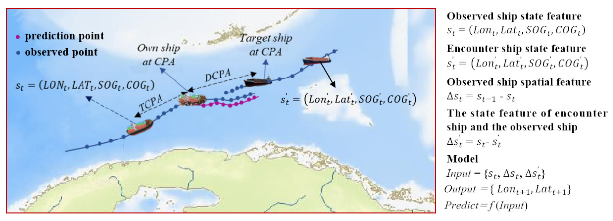
3.1. Problem Statement

During marine traffic encounters, an AIS can obtain the state of interaction between the target ship and the surrounding ships. The state of the ship at time t can be expressed as $s_t=\left(LO{N}_t,LA{T}_t,SO{G}_t,CO{G}_t\right)$, where $LON$, $LAT$, $SOG$ and $COG$ represent longitude, latitude, speed, and heading, respectively. $s_{t-1}-s_t$ represents the change in relative position and state information from t-1 to time t. The spatial position of the encounter ship can be expressed as $s_t^{\prime }$, where $s_t-s_t^{\prime }$ represents the relative position and navigation status information from the encounter ship to the target ship.

As shown in Figure 1, the ship state information at t is used as input to the prediction model, and the location information at t+1 after t is used as the model output. Therefore, we can formulate $\mathit{Output}=\mathit{f}\left(\mathit{Input}\right)$, where $\mathit{f}\left(.\right)$ represents the prediction function of the ship trajectory obtained using our model.

3.2. Methodology Design of Ship Trajectory Prediction

To solve the trajectory prediction of ships in an encounter situation, we add the relative position and navigation status information of the trajectory of the observed ship and the trajectories of the surrounding ships to our prediction framework. In this study, a sequence model is used to determine the impact of the relative positional changes of the observed ship and the ship sailing on the future navigation trajectory of the observed ship. The attention mechanism is used to dynamically adjust the weight of the sequence information to help the model focus on the important position change information, to dynamically adjust the prediction in the sequence prediction process.

This study proposes a new trajectory prediction structure that uses AIS data to train the model, as shown in Figure 2. The model is composed of three modules: Module 1 is an AIS data processing module, which can effectively improve the data quality and model execution efficiency. Module 2 is the trajectory prediction model developed in this study, which is a deep-learning prediction model with an encoder–decoder structure and an attention mechanism. The encoder structure is a multi-layer LSTM, and the decoder consists of an RNN, a multi-layer LSTM, and a self-attention mechanism, which is described in detail in Section 3.3. The training data from Module 1 are used as input to Module 2 to train the prediction model. Finally, Module 3 is a prediction and validation module. Its main function is to apply the test data of Module 1 to optimize the parameters and verify the prediction model of Module 2.

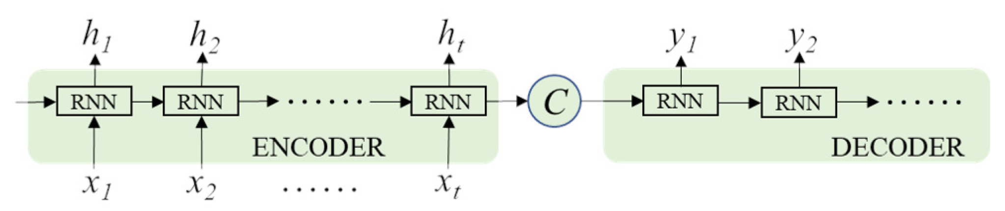
3.3. Design of the Encoder–Decoder Learning Model

The encoder of the proposed model is an LSTM neural network, which maps the input influence onto the sequential context representation. Based on the attention mechanism, the hidden state sequence encoder is combined with the information representation of the context. The decoder of the proposed model is a feature fusion layer that extracts the potential relationships of future ship trajectory state information from the historical and current state information. The weighted representation between the feature vectors of each trajectory is then input into the RNN, so that it can obtain the information representation of the correlation between features in each future prediction step. The RNN in the decoder has a multi-layer structure, to improve the learning ability of the internal sequence information representation. The overall structure is shown in Figure 3.

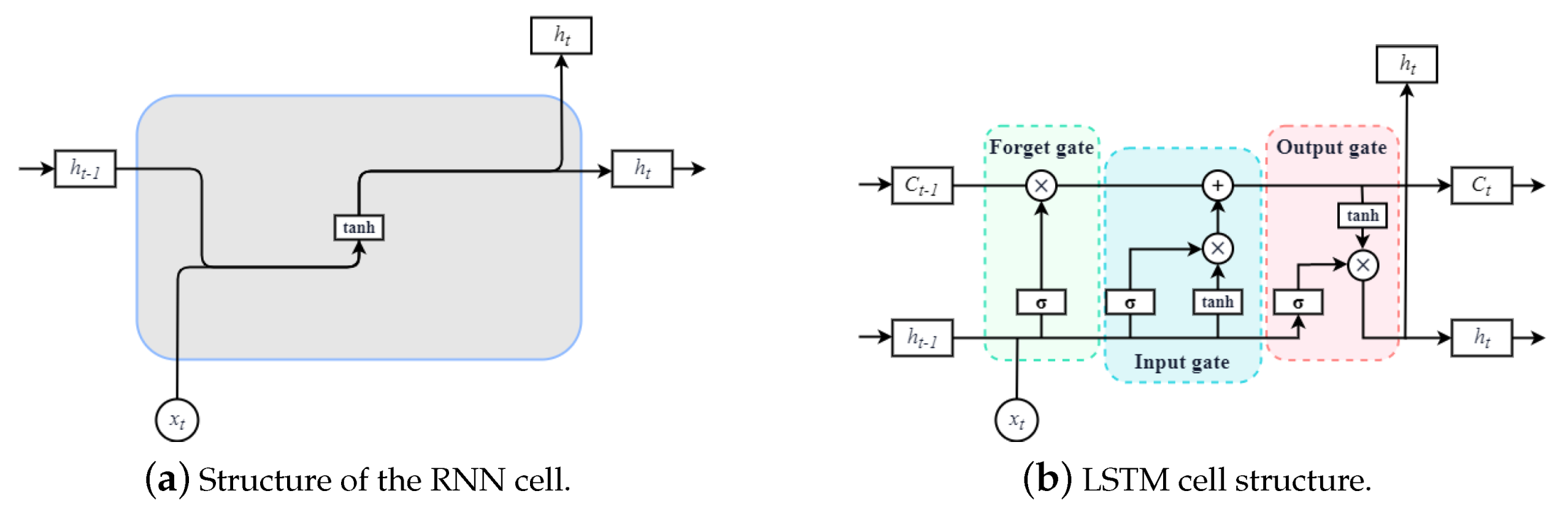
3.3.1. LSTM-Based Sequence to Sequence

The Seq2Seq model consists of an encoder and a decoder. The two units use a recursive neural network (RNN or LSTM) to encode the input as a vector representation and then use another sequential network to decode it. The main task of the encoder is to read the sequence and pass the discovered rules to the decoder. The decoder decodes the received rule information to generate an output sequence.

Figure 4 shows the classic Seq2Seq model architecture.

• $x_1$ to $x_t$ represent the input sequence characteristic information of the model;
• $h_1$ to $h_t$ are the outputs of each circulating neural network cell;
• $y_1$ and $y_2$ represent the label sequence of the model output;
• The variable C between the encoder and decoder represents the sequence information representation obtained by passing the input feature sequence information through the encoder.

The RNN is a feature extractor of global information from the sequence and can be used to process the sequence data. In the RNN, neurons can accept information from other neurons and also their own information, to form a loop structure, as shown in Figure 5a. Here, the gradient disappeared due to the long input sequence.

To solve the problem of the vanishing gradient, a gating mechanism for forgetting the previously accumulated information is required. An LSTM is a type of RNN based on a gating mechanism. Compared with the traditional RNN, an LSTM introduces a gating mechanism to control the speed of information accumulation. Through the forgetting gate, input gate, and output gate, it forgets the previous information and simultaneously adds new information, which effectively solves the loss of learning information caused by a gradient explosion or disappearance. The unit structure is shown in Figure 5b. The notation $\sigma$ represents the sigmoid activation function, $h_{t-1}$ is the output of the previous LSTM unit, $x_t$ indicates the state information of the input at the current time, and $C_{t-1}$ is the internal state of the memory unit in the last moment. Each memory block has three gates to control the path of the information transmission.

a.

Forget gate. $h_{t-1}$, $C_{t-1}$, and $x_t$ are used as inputs to calculate the amount of information $f_t$ (value is between 0 and 1) to be forgotten.

$$f_t=\sigma (W_f·\left[h_{t-1},x_t\right]+b_f)·C_{t-1}$$

(1)

b.

Input gate. The input information $i_t$ and candidate status ${\tilde{C}}_t$ can be obtained by the inputs $h_{t-1}$ and $x_t$ with a sigmoid function and tanh function, respectively. To calculate $i_t·{\tilde{C}}_t$, we need to update the information and forgotten information $C_{t-1}·f_t$, and then obtain a new state $C_t$. The specific Equations are (2)–(4).

$$i_t=\sigma (W_i·\left[h_{t-1},x_t\right]+b_i)$$

(2)

$${\tilde{C}}_t=tanh(W_C·\left[h_{t-1},x_t\right]+b_C)$$

(3)

$$C_t=i_t·{\tilde{C}}_t+C_{t-1}·f_t$$

(4)

c.

Output gate. $h_{t-1}$ and $x_t$ are input to the sigmoid function to obtain the output information $O_t$. The product of the output information and activated value of the current updated state is the information carried by the internal state at the current time $h_t$ as the output information at time t.

$$O_t=\sigma (W_o·\left[h_{t-1},x_t\right]+b_o)$$

(5)

$$h_t=O_t·tanh\left(C_t\right)$$

(6)

Equations (1)–(6) introduce the operation of the LSTM unit in detail. The output function of the LSTM unit can be expressed as follows:

$$h_t=LSTMUnit(x_t,h_{t-1},\theta )$$

(7)

where the LSTMUnit(·) function represents the operation rules forget, input, and output in Equations (1)–(6); and $\theta$ represents the parameters in the LSTM unit.

3.3.2. Attention Mechanism

The attention mechanism module is used in the decoder of the model, to improve the information resource allocation of the model. This can enable the model to dynamically adjust the weights of serial information and allow it to focus on important positions to achieve dynamic adjustment of the weights during the prediction process. The structure of the attention mechanism is shown in Figure 6.

$Keys=values=h_t(t\in \{1,\cdots ,N\})$ are the outputs of all LSTM unit sequences in the encoder at all times, and query = $h^{\prime }$ is the output of the LSTM layer in the decoder. First, the correlation between $h^{\prime }$ and $h_t$ is calculated using the attention-scoring function s$\left(·\right)$. The calculation formula of $h^{\prime }$ is $h^{\prime }=LSTMUnit(X_t,h_t,{\theta }^{{}^{\prime }})$.

The models commonly used as s(·) are additive models, such as point product models or scaling point product models.In this study, a scaling point product model is selected as the score function. It can make better use of a matrix product in the process of matrix operation and can effectively solve the decrease in the softmax function gradient. D represents the dimension of the input vector.

$$s(h_t,h^{\prime })=\frac{h_t^T{h}^{\prime }}{\sqrt{D}}$$

(8)

The softmax function is used to map the output value of the score function between 0 and 1, and the attention distribution of $h^{\prime }$ with respect to $h_t$ is obtained, ${\alpha }_t$, which indicates the degrees of input vector at t. Finally, ${\alpha }_t$ is the weight, and $h_t$ is the weighted sum of the corresponding positions.

$${\alpha }_t=softmax\left(s(h_t,h^{\prime })\right)=\frac{exp\left(s(h_t,h^{\prime })\right)}{{\sum }_{j=1}^{N}exp\left(s(h_j,h^{\prime })\right)}$$

(9)

$$att(H,h^{\prime })=\sum _{t=1}^N{\alpha }_t{h}_t,H=\left[h_1,\cdots ,h_N\right]$$

(10)

3.3.3. Feature Fusion Layer

To model the potential relationships of the ship trajectory information between the historical state and current state, we propose a feature fusion layer. Its structure is shown in Figure 7a. This layer consists of two parts: a multi-layer perceptron (MLP) and a multi-head self-attention (MHSA) mechanism. The MLP is used for linear mapping of the input sequence information. The MHSA is used for calculating and selecting multiple information points from the input information in parallel (see Figure 7b). The original structure of the self-attention mechanism is shown in Figure 6, which is set as Keys = Values = Query. The MHSA can obtain the dependency information at the input stage, connect the input information, and extract the important features from the input data. Simultaneously, these features are spliced with the linear mapping information, which is extracted by the MLP from the input data. The calculation formulas are given as follows:

$$M{H}_{att}=\sigma \left(W_{MH}\left(concat\left(att{\left((K,V),Q\right)}_i\right)\right)\right),fo{r}_{}i=1,\dots ,d$$

(11)

$$M=\sigma \left(W_m·X\right)$$

(12)

$$F=concat\left(M{H}_{att},M\right)$$

(13)

where $\sigma$, $W_{MH}$, and $W_m$ are the activation function in the full connection layer and weight parameters, respectively. The concat$\left(·\right)$ function is used to connect multiple arrays without changing the existing array values. The subscript i of the attention function is the head number of the self-attention mechanism, where K = V = Q = X. Finally, X is the position and status information of the observed ship at time t, the previous k times, and the encounter ship.

4. Numerical Experiments

4.1. Data Description

The AIS data used in this study were mainly collected from onboard AIS equipment in the Yangtze River delta region of China and the eastern coastal region of the United States. In this experiment, we collected a large amount of AIS data and selected six case studies of collision avoidance from the two regions. The research subject data from each region were collected on different dates.

Table 1. Collision avoidance cases of experimental ship trajectories from different areas.

Water Area	MMSI	Number of AIS Points	Date	References
Yangtze River Delta	413450480	2124	1 February 2019	Figure 8a
	413425610	1529
	414386000	912	28 June 2019
	312958000	786
	413556520	257	2 January 2022
	413585000	207
Eastern Coastal Area of the United States	367185680	1440	2 February 2019	Figure 8b
	304604000	823
	372821000	1180	31 December 2021
	311000375	669
	316001635	1112	2 January 2022
	316044371	1440

provides detailed information about the collected data, and Figure 8 shows the specific location of each collision avoidance case.

In the experiment, the navigation trajectory sequence was sequentially sampled with a set sliding window length, where 60% and 40% of the samples were randomly divided into training and testing sets. The processing of experimental datasets for each situation was the same. The training set was used to train and determine the weights, deviation, and other parameters of the model. After training, the test set was used to evaluate the proposed model and other comparison models.

4.2. Setting of Experiments

4.2.1. Criterion of Model Evaluation

The mean square error (MSE) was used as the loss function to quantify the difference between the predicted and real values. After completing the model construction, we used the MAE and average displacement error based on the Haversine distance (HADE) to evaluate the model. These are calculated as follows:

$$MSE=\frac{1}{p}\sum _{l=i}^p{(Y_i-{\widehat{y}}_i)}^2$$

(14)

$$MAE=\frac{1}{p}\sum _{l=i}^p|Y_i-{\widehat{y}}_i|$$

(15)

$$HADE=\frac{1}{p}\sum _{l=i}^{p}2rarcsin\left(\sqrt{{sin}^2\left(\frac{\widehat{la{t}_i}-la{t}_i}{2}\right)+cos\widehat{la{t}_i}cosla{t}_i{sin}^2\left(\frac{\widehat{lo{n}_i}-lo{n}_i}{2}\right)}\right)$$

(16)

where p is the total number of AIS data samples for training or testing, ${\widehat{y}}_i$ is the estimated value of the ship trajectory longitude and latitude, $Y_i$ is the measured value of the navigation longitude and latitude of the ship, r is the Earth’s radius, $\widehat{la{t}_i}$ and $\widehat{lo{n}_i}$ represent the predicted latitude and longitude, and $la{t}_i$ and $lo{n}_i$ represent the true latitude and longitude, respectively. In the experiment, the ship status information containing the first 10 time steps of the current time t was used as input to the model, and the geographic location information of the 10 time steps after the current time t was predicted as the output.

4.2.2. Model Parameter Setting

The Adam adaptive learning rate optimization algorithm [42] was used to update the network parameters of the model structure. In the LSTM layer part of the sequence information extraction, the number of LSTM layers was between one to three. The number of hidden units in each layer of the LSTM searching for the optimal value was taken from [32, 320]. The serial batch size in the experiment was 512, the number of training simulations was 200, and the number of heads for the multi-head self-attention mechanism was 2. To prevent model overfitting, a dropout mechanism [43] and a regularization term were used in the training process. The optimization range and optimization interval granularity of each parameter and the parameter value ranges are shown in

Table 2. Model training parameters.

Parameters	Optimization Range	Interval Granularity	Head-On Situation 1	Head-On Situation 2
Dropout rate	(0.1, 0.5)	0.1	-	-
Learning rate	(0.0001, 0.1)	0.0001	0.002	0.002
No. of LSTM layers	(1, 3)	1	3	3
No. of hidden cells	(32, 320)	32	128	128
No. of MHSA head	(2, 10)	1	2	2
Regularization parameter	(0.01, 1)	0.01	0.001	0.001

. After the comparison experiment with multiple sets of super parameter selection, using the encoder–decoder model based on the multi-module attention mechanism, the parameters of two different trajectory regions (Situation 1 and Situation 2) were chosen as shown in the last two columns of Table 2.

4.2.3. Introduction of Baseline Methods

In the comparisons, we employed four baseline methods, as follows:

(1)

The BPNN has the classic three layers: input layer, hidden layer, and output layer (see Figure 9a). In its network structure, the neurons are connected from the input layer to the output layer;

(2)

LSTM is a classic sequence prediction model. The structure is shown in Figure 9b, and the unit structure of each LSTM cell can be found in Figure 5b;

(3)

DANAE, Denoising automatic encoders (DAE) were proposed by Vincent et al. [44] and are used for prediction tasks, while DANAE is a deep denoising automatic encoder used for attitude estimation [45,46];

(4)

EncDec-ATTN is a deep learning method used for ship trajectory prediction based on recurrent neural networks and was proposed by Capobianco et al. [28]. This method can learn spatiotemporal correlations from historical ship mobility data and predict future ship trajectories.

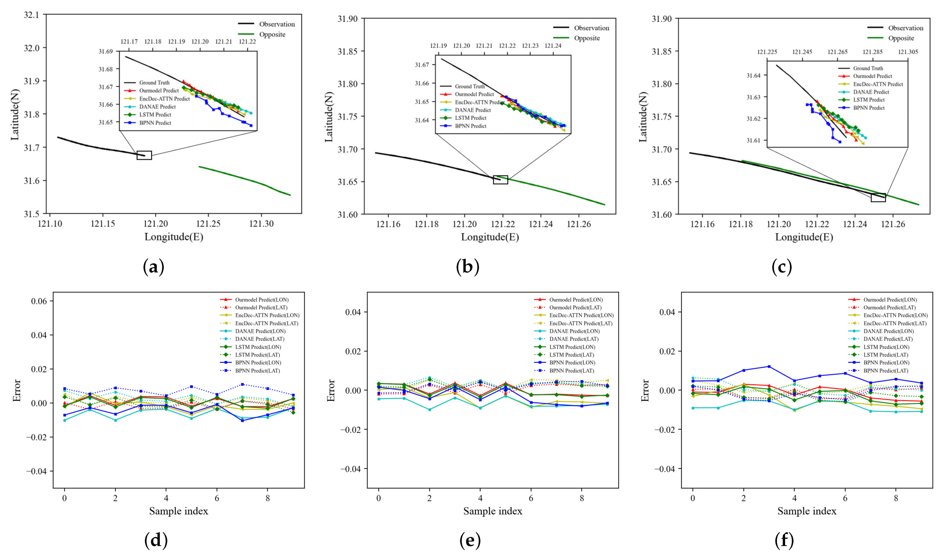
4.3. Prediction Analysis and Result Discussion

4.3.1. Analysis of Model Performance

MSE and MAE were used to evaluate the performance of the model, which was carried out using a Windows 10 system with a 2.90 GHz i5 central processor and 32 GB of memory. The model was coded using TensorFlow 2.4.0 in Python 3.8. The analyses of the prediction performance of our model and those of the other two models are shown in

Table 3. Comparison with the performance index of classic models.

	Model	Position	MSE	MAE	HADE	Optimal Parameter
Head-on Situation 1 from Yangtze River delta	BPNN	LON	3.1854 × ${10}^{-4}$	0.0110	1256.0985	3, (128, 64, 32), 0.01, 0.002
		LAT	3.2575 × ${10}^{-4}$	0.0113
	LSTM	LON	1.4240 × ${10}^{-4}$	0.0093	1072.9199	3, (128, 128, 128), 0.01, 0.002
		LAT	1.5876 × ${10}^{-4}$	0.0096
	DANAE	LON	1.2190 × ${10}^{-4}$	0.0074	890.1905	3, (128, 64, 10), 0.001, 0.002
		LAT	1.5209 × ${10}^{-4}$	0.0085
	EncDec-ATTN	LON	4.5361 × ${10}^{-5}$	0.0051	612.8078	2, (128, 128), 0.002, 0.001
		LAT	5.4565 × ${10}^{-5}$	0.0057
	Our Model	LON	2.5220 × ${10}^{-5}$	0.0041	480.3572	3, (128, 128, 128), 0.002, 0.001
		LAT	2.8857 × ${10}^{-5}$	0.0042
Head-on Situation 2 from eastern coastal area of the United States	BPNN	LON	3.8615 × ${10}^{-4}$	0.0197	1366.2123	3, (128, 64, 32), 0.01, 0.002
		LAT	3.6022 × ${10}^{-4}$	0.0190
	LSTM	LON	1.9693 × ${10}^{-4}$	0.0107	1045.1206	3, (128, 128, 128), 0.01, 0.002
		LAT	1.6729 × ${10}^{-4}$	0.0105
	DANAE	LON	9.1580 × ${10}^{-5}$	0.0077	670.2299	3, (128, 64, 10), 0.001, 0.002
		LAT	9.7660 × ${10}^{-5}$	0.0082
	EncDec-ATTN	LON	5.8020 × ${10}^{-5}$	0.0058	493.7096	2, (128, 128), 0.002, 0.001
		LAT	5.0178 × ${10}^{-5}$	0.0056
	Our Model	LON	3.0541 × ${10}^{-5}$	0.0042	422.7494	3, (128, 128, 128), 0.002, 0.001
		LAT	3.8907 × ${10}^{-5}$	0.0044

.

Table 3 shows that our model had the lowest MSE, MAE, and HADE. In both regions, the parameter number of the LSTM layer was 3, the number of hidden units was 128, the learning rate was 0.002, and the regularization parameter was 0.001. For Head-on Situation 1 from the Yangtze River, the MSE and MAE of the latitude predicted by our model were 2.8857 × ${10}^{-5}$ and 0.0042, respectively, and the MSE and MAE of the longitude were 2.5220 × ${10}^{-5}$ and 0.0041, respectively. For Situation 2 from the eastern coastal area, the MSE and MAE of the latitude predicted by our model were 3.8907 × ${10}^{-5}$ and 0.0044, respectively, and the MSE and MAE of the longitude were 3.0541 × ${10}^{-5}$ and 0.0042, respectively. Comparing with the experimental results of the other models, our model and EncDec-ATTN consistently outperformed the classic network models not using attention mechanisms. Moreover, the evaluation scores of our model decreased by 27.5% and 21.4%, respectively, compared with EncDec-ATTN, which indicated a greater advantage for trajectory prediction in this experiment. HADE reflects the displacement error of the predicted position of a ship from its true position in real scenarios, as shown in Figure 10. In terms of the prediction performance of the ship trajectories, our model had the lowest MSE and MAE values. Meanwhile, the HADE was also lower than that of the other prediction models.

4.3.2. Discussion of the Prediction Results

To further evaluate the prediction ability, a comparison of the prediction results of the different prediction methods at different time steps is shown in Figure 11 and Figure 12. The model prediction was evaluated according to the error between the predicted results and the actual longitude and latitude.

In Head-on Situation 1 from the Yangtze River, as shown in Figure 11a,c, where two ships meet and avoid each other, the first ship is sailing along the planned route, and the course is relatively stable. We observed that all models could predict accurately under relatively simple sailing conditions. As shown in Figure 11b, when the first ship began to change course, the quality of the trajectory prediction generated by our model was much lower than that of the other models.

In Head-on Situation 2 from the eastern coastal region, as shown in Figure 12a–d, during the initial sailing phase with the encounter ship, the first ship encountered the other ship and changed the sailing course. At this time, the prediction results of BPNN, LSTM, and DANAE have large errors. One benefit of the attention mechanism is that our model can predict ship trajectories with less variance from the actual ship trajectories.

In previous studies [28,38,39,40,41], only a single attention mechanism was used to express the historical trajectory and current state information of ships, mainly focusing on hidden information within sequences. However, the correlation of information between the spatiotemporal sequence features is often overlooked. Unlike in previous studies, the proposed model introduces both global attention and multi-head self-attention mechanisms. The global attention mechanism is used to combine the trajectory history and current state information to obtain hidden information between sequences. The multi-head self-attention mechanism can capture the spatiotemporal correlations between the sequence-feature data and extract the fusion features, to generate a new feature representation. The two extracted parts of this information are correlated, to predict the ship trajectory at the next time point.

4.3.3. Analysis of the Attention Mechanism with the Weight Score

Our model includes two attention modules: The global attention mechanism recognizes the information interactions in the input sequence, and the multi-head self-attention mechanism extracts the effective feature information of the output target in the input sequence information. To explore the impact of the attention mechanism on model performance, we compared the performance of the attention mechanism module with and without the attention mechanism, as shown in

Table 4. Comparison of the model performance with and without the attention mechanism.

	Model	Position	MSE	MAE	HADE	Optimal Parameter
Head-on Situation 1 from Yangtze River delta	Seq2Seq	LON	9.0469 × ${10}^{-5}$	0.0075	845.4042	3, (128, 128, 128), 0.01, 0.002
		LAT	9.2702 × ${10}^{-5}$	0.0074
	Seq2Seq-ATTN	LON	5.7978 × ${10}^{-5}$	0.0061	717.5646	3, (128, 128, 128), 0.01, 0.002
		LAT	6.4726 × ${10}^{-5}$	0.0064
	Seq2Seq-MHSA	LON	4.5202 × ${10}^{-5}$	0.0051	608.6507	3, (128, 128, 128), 0.01, 0.002
		LAT	5.2463 × ${10}^{-5}$	0.0055
	Our Model	LON	2.5220 × ${10}^{-5}$	0.0041	480.3572	3, (128, 128, 128), 0.002, 0.001
		LAT	2.8857 × ${10}^{-5}$	0.0042
Head-on Situation 2 from eastern coastal area of the United States	Seq2Seq	LON	9.3664 × ${10}^{-5}$	0.0077	758.1244	3, (128, 128, 128), 0.01, 0.002
		LAT	1.1874 × ${10}^{-4}$	0.0078
	Seq2Seq-ATTN	LON	9.0765 × ${10}^{-5}$	0.0065	629.4445	3, (128, 128, 128), 0.01, 0.002
		LAT	7.0376 × ${10}^{-4}$	0.0058
	Seq2Seq-MHSA	LON	4.6450 × ${10}^{-5}$	0.0050	512.9711	3, (128, 128, 128), 0.01, 0.002
		LAT	5.4739 × ${10}^{-5}$	0.0057
	Our Model	LON	3.0541 × ${10}^{-5}$	0.0042	422.7494	3, (128, 128, 128), 0.002, 0.001
		LAT	3.8907 × ${10}^{-5}$	0.0044

.

Table 4 and Figure 13 show the comparison results of the models under different attention mechanisms. The Seq2Seq model showed a good prediction accuracy with the attention mechanism. Focusing on the prediction for Head-on Situation 1 from the Yangtze River, the prediction results of the model with a global attention mechanism showed decreases in MAE of 0.0014 and 0.0010 in the longitude and latitude predictions, and a decrease in HADE of 15.12%. The MAE of longitude and latitude predicted by the MHSA mechanism decreased by 0.0024 and 0.0019, respectively, and the HADE decreased by 28%. The results of comparing the MSE, MAE, and HADE showed that our model outperformed the other two models with the attention mechanism.

To explain the internal working of the neural network, we obtained the importance weight vector of the input sequence at each position in the prediction sequence and explored the influence of the attention mechanism on the proposed model. Inspired by Lee et al. [47] for the interpretability of the attention mechanism, we visualized the output of two self-attention heads in the prediction model, and the visualization of the output attention weight is shown in Figure 14.

We visualized the weight values calculated by the attention mechanism of the Head-on Situation 2 in the model of different navigation state stages and explained the importance of the network to specific trajectory characteristics. The first column in Figure 14 shows the input, target, and prediction sequences of the different models; the second column shows the visualization of the global attention mechanism weight score of our model, and the last two columns show the visualization of the MHSA weight score of the feature fusion module in our model. In the thermodynamic diagram, the line represents the output sequence, and the list shows the weight distribution of the input sequence. Thus, it can be determined that positions in the history mode are considered more important when generating the predicted trajectory for the global attention mechanism (second column). Over time (from left to right), the model can influence the characteristics of the input sequence when generating the output sequence. At different stages of the predicted navigation status, the positions considered by the output series are different, as shown in Figure 14b,f, which pay more attention to the middle and tail segments of the input series, respectively.

Figure 14j shows a marginal difference in the weight values of the entire series. For the MHSA mechanism (the third and fourth columns), it can be observed from the figures that the different information focused on by the attention head was inconsistent, as shown in Figure 14k. The input ${\mathit{X}}_1$ sequence had a greater correlation with ${\mathit{X}}_1$, ${\mathit{X}}_7$, and ${\mathit{X}}_8$, while ${\mathit{X}}_3$ had a greater correlation with ${\mathit{X}}_4$ and ${\mathit{X}}_9$. The MHSA mechanism calculates the correlation representation between AIS information features and generates a better information feature code for the current input sequence by making full use of the position state information in the sequence. This allows the model to focus on the information of different positions in the input sequence, and it can also alleviate overfitting by integrating different attention heads, to improve the accuracy and robustness of the overall model.

4.3.4. Analysis of Model Validation

For both the Yangtze River delta and eastern coast, we selected two encounter scenarios to verify the effectiveness of the trajectory prediction. Test samples 1 and 2 for the Yangtze River delta contained encounter scenarios of MMSI (414386000, 312958000) on 28 June 2019 and MMSI (413556520, 413585000) on 2 January 2022. Test samples 1 and 2 for the eastern coast contained encounter scenarios of MMSI (372821000, 31100037) on 31 December 2021 and MMSI (316001635, 316044371) on 2 January 2022. The experimental results and comparative analysis are shown in

Table 5. Comparison of the model performance for the test samples.

	Model	Position	Test Sample 1			Test Sample 2
			MSE	MAE	HADE	MSE	MAE	HADE
Yangtze River delta	BPNN	LON	5.5900 × ${10}^{-4}$	0.0137	537.5320	4.7147 × ${10}^{-4}$	0.0217	853.0951
		LAT	5.8601 × ${10}^{-4}$	0.0142		5.1134 × ${10}^{-4}$	0.0226
	LSTM	LON	1.6606 × ${10}^{-4}$	0.0102	399.8864	2.6896 × ${10}^{-4}$	0.0116	640.3072
		LAT	1.7191 × ${10}^{-4}$	0.0108		3.2279 × ${10}^{-4}$	0.0129
	Seq2Seq	LON	8.5295 × ${10}^{-5}$	0.0075	296.0660	9.9816 × ${10}^{-5}$	0.0078	485.1224
		LAT	9.2641 × ${10}^{-5}$	0.0078		1.0563 × ${10}^{-4}$	0.0080
	Seq2Seq-ATTN	LON	7.3838 × ${10}^{-5}$	0.0069	264.7203	8.0580 × ${10}^{-5}$	0.0071	414.3751
		LAT	7.6468 × ${10}^{-5}$	0.0069		8.4536 × ${10}^{-5}$	0.0071
	Seq2Seq-MHSA	LON	5.0014 × ${10}^{-5}$	0.0056	215.3634	6.2602 × ${10}^{-5}$	0.0061	350.034
		LAT	4.4967 × ${10}^{-5}$	0.0055		6.7629 × ${10}^{-5}$	0.0065
	DANAE	LON	1.2231 × ${10}^{-4}$	0.0074	301.2500	1.3935 × ${10}^{-4}$	0.0083	495.0518
		LAT	2.1533 × ${10}^{-4}$	0.0083		8.8652 × ${10}^{-5}$	0.0083
	EncDec-ATTN	LON	5.2074 × ${10}^{-5}$	0.0055	218.4405	5.6014 × ${10}^{-5}$	0.0057	334.0571
		LAT	5.7575 × ${10}^{-5}$	0.0058		7.9404 × ${10}^{-5}$	0.0068
	Our Model	LON	3.2121 × ${10}^{-5}$	0.0044	174.3734	2.9485 × ${10}^{-5}$	0.0044	250.2701
		LAT	3.5942 × ${10}^{-5}$	0.0045		3.5306 × ${10}^{-5}$	0.0048
Eastern Coastal Area of the United States	BPNN	LON	5.4331 × ${10}^{-4}$	0.0233	924.1445	5.2985 × ${10}^{-4}$	0.0160	1356.0606
		LAT	6.2152 × ${10}^{-4}$	0.0249		5.7272 × ${10}^{-4}$	0.0168
	LSTM	LON	1.9752 × ${10}^{-4}$	0.0108	767.8572	1.5630 × ${10}^{-4}$	0.0100	1090.1046
		LAT	2.3233 × ${10}^{-4}$	0.0111		1.3083 × ${10}^{-4}$	0.0097
	Seq2Seq	LON	5.8735 × ${10}^{-5}$	0.0062	586.9804	1.0423 × ${10}^{-4}$	0.0078	880.4276
		LAT	9.7247 × ${10}^{-5}$	0.0076		9.0954 × ${10}^{-5}$	0.0076
	Seq2Seq-ATTN	LON	5.0514 × ${10}^{-5}$	0.0056	520.9248	7.4921 × ${10}^{-5}$	0.0066	745.4695
		LAT	7.4168 × ${10}^{-5}$	0.0068		6.4257 × ${10}^{-5}$	0.0065
	Seq2Seq-MHSA	LON	4.6845 × ${10}^{-5}$	0.0049	383.6337	4.7334 × ${10}^{-5}$	0.0053	621.6424
		LAT	5.7935 × ${10}^{-5}$	0.0059		5.1199 × ${10}^{-5}$	0.0054
	DANAE	LON	9.3591 × ${10}^{-5}$	0.0072	629.2457	1.2319 × ${10}^{-4}$	0.0081	864.9335
		LAT	1.2229 × ${10}^{-4}$	0.0084		9.7121 × ${10}^{-5}$	0.0074
	EncDec-ATTN	LON	4.5829 × ${10}^{-5}$	0.0056	421.0406	5.0587 × ${10}^{-5}$	0.0055	632.9389
		LAT	5.6622 × ${10}^{-5}$	0.0056		4.9324 × ${10}^{-5}$	0.0057
	Our Model	LON	2.9595 × ${10}^{-5}$	0.0043	358.1493	3.2749 × ${10}^{-5}$	0.0043	487.4037
		LAT	4.1747 × ${10}^{-5}$	0.0048		3.5261 × ${10}^{-5}$	0.0042

.

From Table 5, it can be seen that our model achieved the best results for the various evaluation indicators, with the highest accuracy and a good predictive performance. In addition, statistical methods were used to analyze the results, as shown in Figure 15. In terms of the prediction performance of the ship trajectories, our model included an attention module that more effectively extracted important feature information from the trajectory sequences than BPNN, LSTM, Seq2Seq, and DANAE. Compared with the models containing a single attention mechanism, such as Seq2Seq-ATTN, Seq2Seq-MHSA, and EncDec-ATTN, our model effectively extracted correlations between the sequences and features, accounting for multiple attention structures. The experimental results also showed that our model had a good trajectory prediction performance under encounter situations.

5. Conclusions

To predict the future trajectory of a ship in the case of encounter situations, a high-precision trajectory prediction model based on AIS navigation-history data was proposed. This method uses an LSTM neural-network model to encode and decode trajectory information from sequences. The framework of the proposed model uses the relative navigation state information of the encounter and observation ships as part of the input state information characteristics, to predict the observation ship trajectory. Compared with classical models, the proposed model has a stronger generalizability and better performance. Experiments showed that the attention-based model could effectively capture the potential information and correlations in a ship position sequence, so that the proposed model had a better prediction ability for the curve trajectory segment. This significantly improved on the performance of the existing models, which have strong advantages in trajectory prediction. It provides an effective safeguard for ship intelligent navigation systems, by providing real-time trajectory prediction and developing safe and efficient decision support.

In future work, we plan to consider more influencing factors around ships, in the case of multiple ship collisions, and provide further decision support for our model, for more cases of ship collision avoidance.

References

1. Mou, J.M.; van der Tak, C.; Ligteringen, H. Study on collision avoidance in busy waterways by using AIS data. Ocean Eng. 2010, 37, 483–490. [Google Scholar] [CrossRef]
2. Tu, E.; Zhang, G.; Rachmawati, L.; Rajabally, E.; Huang, G.B. Exploiting AIS Data for Intelligent Maritime Navigation: A Comprehensive Survey From Data to Methodology. IEEE Trans. Intell. Transp. Syst. 2018, 19, 1559–1582. [Google Scholar] [CrossRef]
3. Zhu, Y.; Zuo, Y.; Li, T. Modeling of Ship Fuel Consumption Based on Multisource and Heterogeneous Data: Case Study of Passenger Ship. J. Mar. Sci. Eng. 2021, 9, 273. [Google Scholar] [CrossRef]
4. Li, X.; Zuo, Y.; Jiang, J. Application of Regression Analysis Using Broad Learning System for Time-Series Forecast of Ship Fuel Consumption. Sustainability 2023, 15, 380. [Google Scholar] [CrossRef]
5. Cockcroft, A.; Lameijer, J. Part B—Steering and sailing rules. In A Guide to the Collision Avoidance Rules, 7th ed.; Cockcroft, A., Lameijer, J., Eds.; Butterworth-Heinemann: Oxford, UK, 2012; pp. 11–104. [Google Scholar]
6. Huang, Y.; van Gelder, P.; Wen, Y. Velocity obstacle algorithms for collision prevention at sea. Ocean Eng. 2018, 151, 308–321. [Google Scholar] [CrossRef]
7. Lehtola, V.; Montewka, J.; Goerlandt, F.; Guinness, R.; Lensu, M. Finding safe and efficient shipping routes in ice-covered waters: A framework and a model. Cold Reg. Sci. Tech. 2019, 165, 102795. [Google Scholar] [CrossRef]
8. Park, S.W.; Park, Y.S. Predicting Dangerous Traffic Intervals between Ships in Vessel Traffic Service Areas Using a Poisson Distribution. J. Korean Soc. Mar. Environ. Saf. 2016, 22, 402–409. [Google Scholar] [CrossRef]
9. Ristic, B.; La Scala, B.; Morelande, M.; Gordon, N. Statistical analysis of motion patterns in AIS Data: Anomaly detection and motion prediction. In Proceedings of the 2008 11th International Conference on Information Fusion, Cologne, Germany, 30 June–3 July 2008; pp. 1–7. [Google Scholar]
10. Rong Li, X.; Jilkov, V. Survey of maneuvering target tracking. Part I. Dynamic models. IEEE Trans. Aerosp. Electron. Syst. 2003, 39, 1333–1364. [Google Scholar] [CrossRef]
11. Mazzarella, F.; Arguedas, V.F.; Vespe, M. Knowledge-based vessel position prediction using historical AIS data. In Proceedings of the 2015 Sensor Data Fusion: Trends, Solutions, Applications (SDF), Bonn, Germany, 6–8 October 2015; pp. 1–6. [Google Scholar]
12. Ma, X.; Liu, G.; He, B.; Zhang, K.; Zhang, X.; Zhao, X. Trajectory Prediction Algorithm Based on Variational Bayes. In Proceedings of the 2018 IEEE CSAA Guidance, Navigation and Control Conference (CGNCC), Xiamen, China, 10–12 August 2018; pp. 1–6. [Google Scholar]
13. Rong, H.; Teixeira, A.; Guedes Soares, C. Ship trajectory uncertainty prediction based on a Gaussian Process model. Ocean Eng. 2019, 182, 499–511. [Google Scholar] [CrossRef]
14. Barrios, C.; Motai, Y. Improving Estimation of Vehicle’s Trajectory Using the Latest Global Positioning System With Kalman Filtering. IEEE Trans. Instrum. Meas. 2011, 60, 3747–3755. [Google Scholar] [CrossRef]
15. Perera, L.P.; Oliveira, P.; Guedes Soares, C. Maritime Traffic Monitoring Based on Vessel Detection, Tracking, State Estimation, and Trajectory Prediction. IEEE Trans. Intell. Transp. Syst. 2012, 13, 1188–1200. [Google Scholar] [CrossRef]
16. Hexeberg, S.; Flåten, A.L.; Eriksen, B.O.H.; Brekke, E.F. AIS-based vessel trajectory prediction. In Proceedings of the 2017 20th International Conference on Information Fusion (Fusion), Xi’an, China, 10–13 July 2017; pp. 1–8. [Google Scholar]
17. Guo, S.; Liu, C.; Guo, Z.; Feng, Y.; Hong, F.; Huang, H. Trajectory Prediction for Ocean Vessels Base on K-order Multivariate Markov Chain. In Proceedings of the Wireless Algorithms, Systems, and Applications; Chellappan, S., Cheng, W., Li, W., Eds.; Springer International Publishing: Cham, Switzerland, 2018; pp. 140–150. [Google Scholar]
18. Gao, D.W.; Zhu, Y.S.; Zhang, J.F.; He, Y.K.; Yan, K.; Yan, B.R. A novel MP-LSTM method for ship trajectory prediction based on AIS data. Ocean Eng. 2021, 228, 108956. [Google Scholar] [CrossRef]
19. Liu, J.; Shi, G.; Zhu, K. Online Multiple Outputs Least-Squares Support Vector Regression Model of Ship Trajectory Prediction Based on Automatic Information System Data and Selection Mechanism. IEEE Access 2020, 8, 154727–154745. [Google Scholar] [CrossRef]
20. Murray, B.; Perera, L.P. A Data-Driven Approach to Vessel Trajectory Prediction for Safe Autonomous Ship Operations. In Proceedings of the 2018 Thirteenth International Conference on Digital Information Management (ICDIM), Berlin, Germany, 24–26 September 2018; pp. 240–247. [Google Scholar]
21. Valsamis, A.; Tserpes, K.; Zissis, D.; Anagnostopoulos, D.; Varvarigou, T. Employing traditional machine learning algorithms for big data streams analysis: The case of object trajectory prediction. J. Syst. Softw. 2017, 127, 249–257. [Google Scholar] [CrossRef] [Green Version]
22. Zhang, Z.; Ni, G.; Xu, Y. Trajectory prediction based on AIS and BP neural network. In Proceedings of the 2020 IEEE 9th Joint International Information Technology and Artificial Intelligence Conference (ITAIC), Chongqing, China, 11–13 December 2020; Volume 9, pp. 601–605. [Google Scholar]
23. Zhao, Y.; Cui, J.; Yao, G. Online Learning based GA-BP Neural Network to Predict Ship Trajectory. In Proceedings of the 2021 China Automation Congress (CAC), Beijing, China, 22–24 October 2021; pp. 3731–3735. [Google Scholar]
24. Tang, H.; Yin, Y.; Shen, H. A model for vessel trajectory prediction based on long short-term memory neural network. J. Mar. Eng. Technol. 2022, 21, 136–145. [Google Scholar] [CrossRef]
25. Qian, L.; Zheng, Y.; Li, L.; Ma, Y.; Zhou, C.; Zhang, D. A New Method of Inland Water Ship Trajectory Prediction Based on Long Short-Term Memory Network Optimized by Genetic Algorithm. Appl. Sci. 2022, 12, 4073. [Google Scholar] [CrossRef]
26. Ma, H.; Zuo, Y.; Li, T. Vessel Navigation Behavior Analysis and Multiple-Trajectory Prediction Model Based on AIS Data. J. Adv. Transp. 2022, 2022, 6622862. [Google Scholar] [CrossRef]
27. Zhang, X.; Fu, X.; Xiao, Z.; Xu, H.; Qin, Z. Vessel Trajectory Prediction in Maritime Transportation: Current Approaches and Beyond. IEEE Trans. Intell. Transp. Syst. 2022, 23, 19980–19998. [Google Scholar] [CrossRef]
28. Capobianco, S.; Millefiori, L.M.; Forti, N.; Braca, P.; Willett, P. Deep Learning Methods for Vessel Trajectory Prediction Based on Recurrent Neural Networks. IEEE Trans. Aerosp. Electron. Syst. 2021, 57, 4329–4346. [Google Scholar] [CrossRef]
29. Donandt, K.; Böttger, K.; Söffker, D. Short-term Inland Vessel Trajectory Prediction with Encoder-Decoder Models. In Proceedings of the 2022 IEEE 25th International Conference on Intelligent Transportation Systems (ITSC), Macau, China, 8–12 October 2022; pp. 974–979. [Google Scholar]
30. Sutskever, I.; Vinyals, O.; Le, Q.V. Sequence to Sequence Learning with Neural Networks. In Proceedings of the 27th International Conference on Neural Information Processing Systems; MIT Press: Cambridge, MA, USA, 2014; pp. 3104–3112. [Google Scholar]
31. Vaswani, A.; Shazeer, N.; Parmar, N.; Uszkoreit, J.; Jones, L.; Gomez, A.N.; Kaiser, L.; Polosukhin, I. Attention is All You Need. In Proceedings of the 31st International Conference on Neural Information Processing Systems; Curran Associates Inc.: Red Hook, NY, USA, 2017; pp. 6000–6010. [Google Scholar]
32. Hinton, G.E.; Salakhutdinov, R.R. Reducing the Dimensionality of Data with Neural Networks. Science 2006, 313, 504–507. [Google Scholar] [CrossRef] [Green Version]
33. Hochreiter, S.; Schmidhuber, J. Long Short-Term Memory. Neural Comput. 1997, 9, 1735–1780. [Google Scholar] [CrossRef] [PubMed]
34. Chiu, C.C.; Sainath, T.N.; Wu, Y.; Prabhavalkar, R.; Nguyen, P.; Chen, Z.; Kannan, A.; Weiss, R.J.; Rao, K.; Gonina, E.; et al. State-of-the-Art Speech Recognition with Sequence-to-Sequence Models. In Proceedings of the 2018 IEEE International Conference on Acoustics, Speech and Signal Processing (ICASSP), Calgary, AB, Canada, 15–20 April 2018; pp. 4774–4778. [Google Scholar]
35. Forti, N.; Millefiori, L.M.; Braca, P.; Willett, P. Prediction oof Vessel Trajectories From AIS Data Via Sequence-To-Sequence Recurrent Neural Networks. In Proceedings of the 2020 IEEE International Conference on Acoustics, Speech and Signal Processing (ICASSP), Barcelona, Spain, 4–8 May 2020; pp. 8936–8940. [Google Scholar]
36. Bahdanau, D.; Cho, K.; Bengio, Y. Neural Machine Translation by Jointly Learning to Align and Translate. In Proceedings of the 2015 3rd International Conference on Learning Representations (ICLR), San Diego, CA, USA, 7–9 May 2015. [Google Scholar]
37. Luong, T.; Pham, H.; Manning, C.D. Effective Approaches to Attention-based Neural Machine Translation. In Proceedings of the 2015 Conference on Empirical Methods in Natural Language Processing; Association for Computational Linguistics: Lisbon, Portugal, 2015; pp. 1412–1421. [Google Scholar]
38. Jiang, D.; Shi, G.; Li, N.; Ma, L.; Li, W.; Shi, J. TRFM-LS: Transformer-Based Deep Learning Method for Vessel Trajectory Prediction. J. Mar. Sci. Eng. 2023, 11, 880. [Google Scholar] [CrossRef]
39. Altan, D.; Marijan, D.; Kholodna, T. SafeWay: Improving the safety of autonomous waypoint detection in maritime using transformer and interpolation. Marit. Transp. Res. 2023, 4, 100086. [Google Scholar] [CrossRef]
40. Jiang, J.; Zuo, Y. Prediction of Ship Trajectory in Nearby Port Waters Based on Attention Mechanism Model. Sustainability 2023, 15, 7435. [Google Scholar] [CrossRef]
41. Capobianco, S.; Forti, N.; Millefiori, L.M.; Braca, P.; Willett, P. Recurrent Encoder—Decoder Networks for Vessel Trajectory Prediction With Uncertainty Estimation. IEEE Trans. Aerosp. Electron. Syst. 2023, 59, 2554–2565. [Google Scholar] [CrossRef]
42. Kingma, D.P.; Ba, J. Adam: A method for stochastic optimization. In Proceedings of the 2015 3rd International Conference on Learning Representations (ICLR), San Diego, CA, USA, 7–9 May 2015. [Google Scholar]
43. Srivastava, N.; Hinton, G.; Krizhevsky, A.; Sutskever, I.; Salakhutdinov, R. Dropout: A Simple Way to Prevent Neural Networks from Overfitting. J. Mach. Learn. Res. 2014, 15, 1929–1958. [Google Scholar]
44. Vincent, P.; Larochelle, H.; Bengio, Y.; Manzagol, P.A. Extracting and Composing Robust Features with Denoising Autoencoders. In Proceedings of the 25th International Conference on Machine Learning; Association for Computing Machinery: New York, NY, USA, 2008; pp. 1096–1103. [Google Scholar]
45. Russo, P.; Ciaccio, F.D.; Troisi, S. DANAE: A denoising autoencoder for underwater attitude estimation. In Proceedings of the 2020 IMEKO TC-19 International Workshop on Metrology for the Sea, Naples, Italy, 5–7 October 2020; pp. 195–198. [Google Scholar]
46. Russo, P.; Di Ciaccio, F.; Troisi, S. DANAE++: A Smart Approach for Denoising Underwater Attitude Estimation. Sensors 2021, 21, 1526. [Google Scholar] [CrossRef]
47. Lee, J.; Shin, J.H.; Kim, J.S. Interactive Visualization and Manipulation of Attention-based Neural Machine Translation. In Proceedings of the 2017 Conference on Empirical Methods in Natural Language: System Demonstrations, Copenhagen, Denmark, 9–11 September 2017; Association for Computational Linguistics: Copenhagen, Denmark, 2017; pp. 121–126. [Google Scholar]
Figure 1. Overview explanation of trajectory prediction.
Jmse 11 01530 g001
Figure 2. Overview of the proposed trajectory prediction model.
Jmse 11 01530 g002
Figure 3. Overview of our model.
Jmse 11 01530 g003
Figure 4. Seq2seq model architecture.
Jmse 11 01530 g004
Figure 5. Structure of the recurrent neural network cell. The symbol x t represents the input information of the RNN at the current time step t, h t 1 represents the hidden state of time step t − 1, and h t represents the output information of time step t.
Jmse 11 01530 g005
Figure 6. Attention mechanism structure.
Jmse 11 01530 g006
Figure 7. Structure of the feature fusion layer and multi-head attention mechanism.
Jmse 11 01530 g007
Figure 8. Two routes of the case ships; the red line represents the navigation trajectory of the observation ship; the black line represents the navigation trajectory of the opposite ship. (a) Navigation trajectory of collision avoidance for ships in Yangtze River delta. (b) Navigation trajectory of collision avoidance for ships in the eastern coastal area of the United States.
Jmse 11 01530 g008
Figure 9. The basic structure of the baseline method.
Jmse 11 01530 g009
Figure 10. Results comparison of the MSE, MAE, and HADE. Brown and blue-green represent the evaluation indicators for Situations 1 and 2 from different areas, respectively. The green dots represent the average values.
Jmse 11 01530 g010
Figure 11. The prediction results for Head-on Situation 1. (ac) Visualization of ship navigation trajectory predicted at different time steps. (df) Error of predicted navigation trajectory at different time steps. The "ground truth" in the legend represents the true values of the experimental sample.
Jmse 11 01530 g011
Figure 12. The prediction results for Head-on Situation 2. (ac) Visualization of the ship navigation trajectory predicted at different time steps. (df) Error of the predicted navigation trajectory at different time steps. The “ground truth” in the legend represents the true values of the experimental sample.
Jmse 11 01530 g012
Figure 13. Comparison results of MSE, MAE, and HADE. Brown and blue-green represent the evaluation indicators for Situations 1 and 2 from different areas, respectively. The green dots represent the average value.
Jmse 11 01530 g013
Figure 14. Weights of attention mechanism. (a,e,i) is the prediction results of the ship navigation trajectory at different conditions. (b,f,j) Weights of the global attention mechanism. (c,g,k) and (d,h,l) represent the weight values of the self-attention mechanism for the two heads, respectively.
Jmse 11 01530 g014
Figure 15. Comparison analysis of the MSE, MAE, and HADE of the test samples from the different areas. Brown and blue-green boxplots represent the evaluation indicators for test samples 1 and 2, respectively. The green dots are the average value. Figure (ae) and (fj) represent the Yangtze River and eastern coastal area, respectively.
Jmse 11 01530 g015