Abstract
In the shipping network optimization, the feeder liner companies not only need to decrease the operation cost by comprehensively optimizing the route, schedule, and fleet but also try to increase the operation income by attracting more shippers, with multimodal transport-path selection considered. Therefore, this paper proposes the integrated planning of feeder route selection, schedule design, and fleet allocation with shippers’ transport-path selection considered. We utilize the nested Logit model to analyze the shipper selection behavior for the multimodal transport path and then formulate a mixed-integer nonlinear programming model of integrated optimization for route, schedule, and fleet. To solve our nonlinear model, we propose a particle swarm optimization (PSO) framework embedded with CPLEX solver by combining the constraint relaxations and the linearization techniques with the heuristic rules. Based on the multimodal transport system in Northern China, computational experiments were conducted to verify the effectiveness of our model and algorithm. The sensitivity analyses of model parameters show that with the increase in ship rent, feeder liner companies should reduce the ship capacity or try to increase the number of port call. With the increase in fuel price, feeder liner companies should reduce the ship speed under the constraints of the arrival-time window and schedule interval. If shippers’ time utility coefficient is high, feeder liner companies should shorten the sailing time of ships by decreasing the number of port calls or shorten the at-port time of ships by increasing the service frequency. If the multimodal transport paths are cost-advantaged or if the waterway transport time has a small impact on multimodal transport time, feeder liner companies should weigh the increase in income and cost when using the measures of time saving. These management insights provide decision support for the operation practice of liner shipping network optimization.
1. Introduction
Maritime transport undertakes the majority of intercontinental trade. Liner shipping is the most widely used method of transporting container goods in maritime transport [1]. According to the UNCTAD report on maritime transportation 2020, there are 152 million twenty-foot containers and about 5200 containerships worldwide [2]. Container liner shipping relies on the network structure with trunk and feeder routes. Large ships sail between the trunk ports worldwide in the trunk liner shipping, while small and medium ships shuttle between the trunk ports and regional feeder ports, namely the feeder liner shipping [3]. Compared to feeder liner shipping, the trunk liner shipping has richer achievements in practice and theory [4]. However, feeder liner shipping plays an important role in improving the trunk and feeder network, as well as the inland multimodal transport network. In addition, feeder liner shipping has an important impact on the transport time and freight rate of container transportation [5,6]. Therefore, this paper focuses on the shipping network optimization of feeder liner transport.
The liner shipping company publishes information in advance, up to three months, on port calls, port rotation, service frequency, arrival time, and freight rate, so that shippers can reasonably arrange production, transportation, and distribution plans [4,7]. To decrease the operation cost under the premise of maintaining regular transport services, the liner shipping company should comprehensively consider the three factors, i.e., route, schedule, and fleet, that simultaneously affect the operation cost [2]. For example, the number of port calls determines the round-trip time and influences the service frequency. In addition, the number of port calls determines the ship capacity and directly affects the ship quantity. Thus, we need to engage in integrated planning of route selection, schedule design, and fleet allocation to maximize operation cost savings [7].
In addition to the decrease in the operation cost, it is also important for liner shipping companies to increase operation income by attracting more shippers and demand. The transport-path selection and container transportation demand were often assumed to be fixed in previous studies. In fact, the container transportation demand fluctuates, as shippers will select the transport path based on their preferences [8]. Shippers would select the transport path with favorable freight rate or transport time, which leads to an increase in the container transportation demand on the transport path. In order to increase the operation income, the liner shipping company should shorten the sailing time of ships by decreasing the number of port calls or reduce the at-port time of ships by increasing the service frequency. In addition, the liner shipping company can reduce the freight rate appropriately to attract shippers to select transport paths. In other words, the shippers’ transport-path selection should be considered in the liner shipping network optimization [9,10].
This paper introduces the shippers’ transport-path selection to the integrated planning of route selection, schedule design, and fleet allocation. There are two different aspects between our problem and the previous studies. First, most research on liner shipping focuses on the trunk routes, as well as the trunk and feeder network [4,6], while this paper extends above studies to the feeder shipping network. In addition, previous papers often explored one item of route selection, schedule design, and fleet allocation, while we address the integrated optimization for route, schedule, and fleet. Second, previous liner shipping studies seldom consider the shippers’ transport-path selection [10], which is explored in this paper. In addition, the previous transport-path selection was aimed at the port-to-port-based liner shipping routes. However, the road transport and rail transport also carry a container freight, which forms the multimodal transport together with liner shipping. Thus, we extended the previous studies on the door-to-door-based multimodal transport-path selection.
The main contributions of this paper are as follows: (i) We propose the integrated planning of route selection, schedule design, and fleet allocation with shippers’ transport-path selection considered. (ii) The nested Logit model is used to analyze the multimodal transport-path selection. Then, we formulate a mixed-integer nonlinear programming model of integrated optimization for route, schedule, and fleet. (iii) A particle swarm algorithm (PSO) framework embedded with CPLEX solver is designed by combining the constraint relaxations and the linearization techniques with the heuristic rules.
This paper is organized as follows: Section 2 presents the literature review on the feeder shipping network optimization and the shippers’ selection behavior analysis. Section 3 introduces the shippers’ multimodal transport-path selection and then describes the integrated planning of route selection, schedule design, and fleet allocation. Section 4 establishes an integrated optimization model for route, schedule, and fleet, considering transport-path selection. Section 5 designs a PSO framework embedded with CPLEX and then presents the algorithm flow and main steps. In Section 6, the computational experiments are conducted based on the multimodal transport system in Northern China for the effectiveness validation and the sensitivity analysis. Section 7 summarizes the research contributions and prospects of this study.
2. Literature Review
Here, we present research on feeder shipping network optimization and shippers’ transport-path selection to summarize the research progress and the difference with this study.
2.1. Feeder Shipping Network Optimization
As for the research on the feeder shipping network optimization, Polat et al. [11] compared three feeder shipping network schemes for a short-haul liner shipping company in Black Sea region and proposed a mixed-integer linear programming model, as well as an adaptive neighborhood-search algorithm. Zheng and Yang [12] addressed the hub-and-spoke shipping network design along the Yangtze River. Santini et al. [3] proposed a branch-and-price approach for solving the feeder shipping network design with variable ship speed. Krile [13] addressed a routing problem of small island ports to decide the order of attachment of each island and provide an appropriate time schedule. A network optimization methodology that linked minimal transport cost and maximal revenue was proposed to avoid the complex and time-consuming computations due to nonlinear polynomial optimization. However, this methodology cannot address the fleet allocation and speed optimization at the same time. Lin et al. [14] developed a multi-objective optimization for the feeder shipping network at Kotka port, considering the cost, income, equipment usage, round-trip time, and competitiveness. Msakni et al. [4] analyzed the impact of network structures on operation cost for a real case in Norwegian and European continental ports. Paolo et al. [15] optimized the Ro-Ro shipping network to improve the service level in the Mediterranean region by using the two-hub-based scheme instead of the multi-port-calling scheme. Koza et al. [16] proposed a joint optimization for route and schedule with the constraints of variable ship speed, committed arrival time, and specific network structure. Hellsten et al. [17] proposed an adaptive neighborhood-search algorithm to solve the feeder shipping network design model. Hellsten et al. [1] formulated a vehicle routing optimization model with specific service frequency and simultaneous pickup-and-delivery characteristics for the feeder liner shipping network design. Medić et al. [18] developed a trunk-and-feeder network optimization method to address the case in the Adriatic Sea. In their study, they determined the trunk port by using multicriteria decision-making and an expert evaluation method and then optimized the feeder routes by using the traveling-salesman algorithm. Zhu et al. [19] formulated a barge allocation and scheduling model with the objective of minimizing carbon emissions and then proposed a variable neighborhood-search algorithm. Jin et al. [6] proposed the feeder routing and scheduling problem at a congested hub port, and it was solved by the branch-and-pricing algorithm and column-generation algorithm. Corey et al. [20] studied the hub-port location and feeder-port allocation problem with the objective of improving container transshipment potential in the Caribbean Sea and formulated two mixed-integer linear programming models with single allocation and multiple allocation. Zhou et al. [21] explored an integrated planning in the inland river hub-and-spoke network, including the hub port selection, feeder port allocation, and fleet deployment. It is not difficult to find that there are few studies on the integrated optimization for feeder route, schedule, and fleet. Our study can help fill this research gap.
2.2. Shippers’ Transport-Path Selection
Some studies have focused on the impact of shippers’ selection on liner shipping routes. We present the consideration of shippers in these studies and distinguish whether they are door-to-door in Table 1. Chen et al. [22] addressed the liner shipping network optimization based on the traffic-flow allocation model, considering the interaction between network design and freight demand. Wang et al. [23] analyzed the impact of shippers’ route selection on the shipping route and pricing scheme, with the transport time and freight rate considered. Kashiha et al. [24] found that there are different factors influencing shippers’ route selection in the European coastal and inland countries. Yang et al. [25] proposed a bi-level programming model for the shipping network reconstruction problem, where the upper model was to maximize the operation revenue of liner companies and the lower model minimized the transport cost of shippers. Tu et al. [9] proposed a gravity-model-based OD demand forecast method and then formulated one shipping network optimization model to maximize total social welfare. Duan et al. [26] analyzed the shippers’ shipping-route selection based on time value and reliability value and proposed one network design model with transshipment and ship capacity considered. Jiang et al. [27] optimized the near-sea liner shipping network faced to the big customers’ preferences on ship arrival time by taking into account the operation cost of ships and the penalties of late arrival. Chen et al. [28] formulated a China–West Africa shipping network design model with shippers’ transport-path selection considered, facing the future prospect of more frequent China–West Africa trade. Zeng et al. [29] analyzed the market share of Arctic shipping over the Suez Canal and China–Europe railway, considering freight rate, transport time, cargo damage, and convenience. Cheng and Wang [10] proposed one shipping-network optimization model to maximize the operation revenue of liner companies by taking into account shippers’ inertia preference for brand effect and non-inertia preference for transport time and freight rate. Gao et al. [30] formulated a bi-level programming model with carbon-tax policy and shipper preferences considered for the joint optimization of ship route and schedule. Du et al. [8] proposed a liner shipping schedule design model considering shipper selection behavior and time-window constraint to explore the shipper selection behavior by considering the brand effect, transport time, freight rate, and ship arrival time. Most research studies focus on the port-to-port-based shipping-route selection, which does not apply in reality when a large amount of container transport demands is door-to-door-based multimodal transport. We focus on the door-to-door-based multimodal transport-path selection in this paper.

Table 1.
Overview of studies on transport-path selection.
3. Problem Description
Here, we first introduce the shipper selection behavior for the multimodal transport path and propose a nested Logit model for the transport-path selection. Then, we present the feeder route selection, schedule design, and fleet allocation, respectively, in the feeder shipping network optimization.
3.1. Notations
Sets:
is the set of multimodal transport path, and is the total number of multimodal transport paths.
is the set of feeder ports, and is the total number of feeder ports. In addition, Port 0 is set as the trunk port.
is the set of feeder routes, and is the total number of feeder routes.
is the set of feeder ships, and is the total number of feeder ships.
Parameters:
: the weekly transportation demand from the inland origin of multimodal transport path . and are the export demand and import demand, respectively.
: the road distance on multimodal transport path .
: the railway distance on multimodal transport path .
: the freight rate of the feeder liner on multimodal transport path .
: the freight rate of the trunk liner on multimodal transport path .
: the freight rate of the whole multimodal transport path .
: the railway transit period on multimodal transport path .
: the committed transport time of the trunk liner on multimodal transport path .
: the unit freight rate of road transport.
: the base price I of rail transport.
: the base price II of rail transport.
: the average speed of road transport.
: the utility coefficient of shippers for brand effect on multimodal transport path .
: the utility coefficient of shippers for freight rate on multimodal transport path .
: the utility coefficient of shippers for transport time on multimodal transport path .
: the random utility of shippers for brand effect.
: the random utility of shippers for transport time and freight rate.
: equal to one when feeder port belongs to feeder route . Otherwise, is equal to zero.
: the weekly service frequency on feeder route .
: the total sailing mileage of ships on feeder route .
: the sailing mileage from feeder port to feeder port on feeder route .
: the sailing mileage from feeder port to feeder port on feeder route .
: the capacity of feeder ship .
: the full load limit of feeder ships.
: the minimum speed of feeder ships.
: the maximum speed of feeder ships.
: the schedule interval of the trunk liner.
: the arrival-time window of ships at the trunk port.
: the container handling efficiency at each port.
: daily ship rent for the unit capacity.
: the port charge of ships per trip.
: the container handling fee per TEU.
: the fuel-consumption rate of ships when sailing at sea.
: the fuel-consumption rate of ships when working at port.
: the carbon emissions cost of fuel consumption, which represents the carbon tax.
: the multimodal transport subsidy.
: the fuel price of ships.
Auxiliary variables:
: the transport time of the whole multimodal transport path .
: the transport time of the feeder liner on multimodal transport path .
: the utility value of shippers for brand effect on multimodal transport path .
: the path-selection ratio of shippers for brand effect on multimodal transport path .
: the utility value of shippers for transport time and freight rate on multimodal transport path .
: the path-selection ratio of shippers for transport time and freight rate on multimodal transport path .
: the path-selection ratio of shippers for brand effect, transport time, and freight rate on multimodal transport path .
: the weekly transportation demand between feeder port and trunk port 0 on feeder route . The parameters and are the export demand and import demand, respectively.
: the container volume when ships leaving trunk port 0 on feeder route .
: the container volume when ships leaving feeder port on feeder route .
: the maximum container volume when ships leaving port on feeder route .
: the total at-port time of ships on feeder route .
: the total sailing time of ships on feeder route .
: the ship quantity on feeder route .
: the rent cost of ships on feeder route .
: the at-port cost of ships on feeder route .
: the sailing cost of ships on feeder route .
: the carbon emission cost on feeder route .
: the multimodal transport subsidy on feeder route .
: the weekly operation cost on feeder route .
: the weekly operation income on feeder route .
: the weekly operation revenue of the feeder shipping network.
Decision variables:
: the binary variable for route selection. equals 1 when feeder route is selected; otherwise, equals 0.
: the binary variable for fleet allocation. is equal to 1 when feeder ship is allocated to feeder route ; otherwise, is equal to 0.
: the ship speed on feeder route .
3.2. Shipper Selection Behavior for the Multimodal Transport Path
3.2.1. Multimodal Transport-Path Selection
Intercontinental trades often use door-to-port-based multimodal transport. The multimodal transport often includes road transport, rail transport, water transport, and sea transport. Different transport modes and paths make up various multimodal transport paths. The shipper of the seller organizes the multimodal transport from the inland origin to the oversea port, while the shipper of the buyer is responsible for the other transport processes from the oversea port to the inland destination. In the literature on multimodal transport, the container transportation demand is often fixed, and the inland transport path and the waterway port are often determined [31]. In fact, since shippers select the multimodal transport path based on their preferences, the transportation demand and the feeder port will change with it [32].
An illustration of multimodal transport paths is shown in Figure 1 to show that the container transportation demand is allocated to these multimodal transport paths via shipper selection behavior. Note that all paths are assigned container demand without path selection. In this figure, the inland transportation demands from Hulunbeier, Wulumuqi, Xi’an, and Changsha need to gather at Shanghai port and then are transported to Canada and the west coast of the United States via trunk liner shipping. In the multimodal transport-path selection, the shippers in Xi’an can select long-distance road transport or road–water transport via the Yangtze River, and the shippers in Hulunbeier can select long-distance rail transport or road–water transport via the Dalian–Shanghai feeder liner. Note that a multimodal transport path is a combination of some specific paths instead of the arbitrary combination of road path, rail path, and waterway route [33]. In this paper, we provide a set of multimodal transport paths for selection. Then, the container transportation demand will be allocated to these multimodal transport paths via shipper selection behavior.
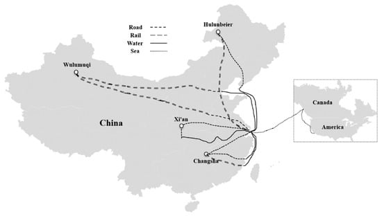
Figure 1.
Container transportation demand allocation on multimodal transport paths.
3.2.2. Shippers’ Inertia and Non-Inertia Preferences
The shipper preferences for transport-path selection can be classified into inertia and non-inertia preferences [10,30]. The inertia preference refers to shippers’ transport-path selection based on their habits, whose main influencing factor is brand effect [34,35,36]. The non-inertia preference refers to shippers’ transport-path selection via the comparison of transportation plans, affected by transport time, freight rate, ship arrival time, risk, stability, etc. [10,23,26,27,37]. This paper introduces the shippers’ inertia and non-inertia preferences into the transport-path-selection analysis, where the brand effect, the freight rate, and the transport time of each multimodal transport path are evaluated.
With export and import directions, the multimodal transport path consists of the road transport, rail transport, water transport (feeder liner), and sea transport (trunk liner). The freight rate and transport time of the whole multimodal transport path are calculated by Formulas (1) and (2). In Formula (1), the freight rate of road transport needs to multiply unit freight rate by road distance, the freight rate of rail transport needs to multiply base price II by rail distance on the basis of base price I, and the freight rates of feeder liner and trunk liner are given in advance. In Formula (2), the road transport time needs to divide by road distance by the average speed, the rail transport time equals the railway transit period, and the sea transport time equals the committed transport time of the trunk liner.
In the above formulas, the road distance and unit freight rate, the railway transit period and base price, the freight rate of the trunk liner and feeder liner, and the committed transport time of the trunk liner can be collected via internet. The freight rate of the feeder liner, , depends on the sailing mileage of ships between feeder port and trunk port, and it is slightly affected by the service frequency, port call, and port rotation. Moreover, the service frequency, port call, and port rotation directly determine the transport time of the feeder liner, . According to the container transshipment time and the at-port time and sailing time of ships, we can calculate the transport time, , in export and import directions by Formulas (3) and (4). In these two formulas, the container transshipment time is defined as the half of schedule interval [31], so it is expressed as . Moreover, is the accumulated mileage from feeder port to the trunk port on feeder route , and is the accumulated mileage in the opposite direction.
3.2.3. Nested Logit Model for Transport-Path Selection
To analyze the transport-path selection, a nested Logit model is proposed, where the inertia and non-inertia preferences are separated into two layers. The nested Logit model overcomes the IIA property in the polynomial model by making the alternatives in the same layer related, while the alternatives in different layers independent [8,10,38]. The tree structure with two layers of the nested Logit model is shown in Figure 2. The first layer selects multimodal transport carriers according to brand effect, and the second layer selects a multimodal transport path according to the freight rate and transport time. Then, we can evaluate the shippers’ utility value and calculate the path-selection ratio for the multimodal transport carriers and paths, respectively. If the freight rate and transport time of multimodal transport path are relatively favorable, the path-selection ratio may be low due to the poor brand effect. This selection process based on the nested Logit model is consistent with the container transport practice.
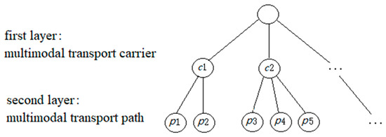
Figure 2.
The tree structure of nested Logit model.
The nested Logit model for the transport-path selection can be described as Formulas (5)–(10). Formula (5) evaluates the shippers’ utility value for brand effect on multimodal transport path . Formula (6) calculates the shippers’ selection ratio for brand effect on multimodal transport path . For the utility function of Formula (7), as the shippers prefer the lower freight rate and the shorter transport time, the freight rate and transport time are in the denominator of utility function [8,38]. Formula (8) calculates shippers’ selection ratio for freight rate and transport time on multimodal transport path . Formula (9) calculates the shippers’ selection ratio for brand effect, freight rate, and transport time on multimodal transport path . Formula (10) allocates the container transportation demand to each multimodal transport path and then determines the export demand, , and import demand, , on multimodal transport path . It is worth noting that the utility coefficients in the formulas are known parameters that can be calibrated through RP/SP surveys [29,39], or valued in reference to the container transport market [8,23]. The two random utilities follow the double exponential distribution [38], representing the influence of unknown factors on the shippers’ transport-path selection.
3.3. Integration Planning of Route Selection, Schedule Design, and Fleet Allocation
3.3.1. Planning of Route Selection
Although the road path, rail path, feeder port, and trunk port on the multimodal transport path are given, the port calls and port rotation on each feeder route still have an influence on the transport time, which may affect the transport-path-selection ratio. For example, the direct route between trunk port and feeder port has a shorter transport time compared with the multi-port route.
There are currently two ways to describe the feeder route, i.e., the network design problem generated from scratch [7,12,40,41,42] and the route selection problem based on given schemes [4,25,43,44,45]. As the number of port calls and feeder routes is limited, we carry out the route comparison based on given schemes.
Based on the given set of feeder routes, , we can easily provide the port calls, ; the service frequency, ; and the sailing mileage, , on each feeder route. To be consistent with the container transport practice, we require that each feeder port needs to be served by only one feeder route, which can be expressed as Formula (11).
3.3.2. Planning of Schedule Design
After determining the port call and port rotation, we can calculate the at-port time, , and the sailing time, , on feeder route . The at-port time of ships depends on the container transportation demand and the handling efficiency, which can be calculated by Formula (12). Since each container needs to be loaded and unloaded, the handling volume in Formula (12) is two times the container transportation demand. Considering that the service frequency may exceed once one week, the handling volume in Formula (12) needs to be divided by service frequency. The sailing time of ships depends on the sailing mileage and the ship speed, as shown in Formula (13). The ship speed in Formula (13) is the decision variable, which has the influence on the round-trip time of ships. The ship speed is constrained by Formula (14) to ensure that it will not lose power due to low speed and will not damage the engine due to high speed.
Based on the at-port time and sailing time of ships, we can calculate the round-trip time, , by using Formula (15). This round-trip time is the length of time consumed by a ship to complete its transport task and return to the trunk port. The round-trip time is related to the transshipment process between trunk liner and feeder liner, which is an important constraint of feeder shipping network optimization [14]. The transshipment process is consistent with the practical operation, which can make the calculation results easier to be applied in practice. Formula (16) restricts the round-trip time, , of the feeder liner so that it cannot exceed the schedule interval, , of the trunk liner. Formula (16) indicates that feeder ships need to return before the trunk ship departs. Formula (17) requires that the arrival time of each round trip , needs to satisfy the arrival-time window, , at the trunk port. Formula (17) represents that there are available berths when feeder ship returns to the trunk port [8,46].
3.3.3. Planning of Fleet Allocation
Based on the given set of feeder ships, , we need to determine the ship quantity. Specifically, Formula (18) ensures that each feeder ship can be allocated to, at most, one feeder route, and Formula (19) can calculate the ship quantity, , allocated to feeder route . In addition, the ship quantity required can be determined by the round-trip time and service frequency. Formula (20) requires that the ship quantity, , that is allocated satisfies the ship quantity required.
In addition to the ship quantity allocated, we need to calculate the ship capacity according to the container handling volume. Specifically, the container volume at the trunk port is 0, and it needs to load all of the import demand. Then, the container volume at feeder port can be obtained after unloading the export demand, , and loading import demand, . Formula (21) can determine the maximum container volume when ships leave port on feeder route , where the parameter is the known full load limit of the feeder ship. Formula (22) requires the maximum container volume, , to not exceed the capacity of the feeder ship, .
3.3.4. Integrated Optimization for Route, Schedule, and Fleet
In the feeder shipping network optimization, there are mutual influences between the decision variables of route, schedule, and fleet. We provide objective, input, and decision for three subproblems in Table 2 and show the relationship between three subproblems in Figure 3. For example, the number of port calls determines the round-trip time of ships, and it has an influence on the ship quantity allocated to the feeder route. The port rotation determines the container volume when ships leave port, and it has an influence on the ship capacity allocated to the feeder route. The service frequency determines the ship quantity, and it also affects the transshipment time at feeder ports. The ship speed determines the sailing time and round-trip time of ships, and it also affects the ship quantity.
Table 2.
Objective, input, and decision for three subproblems.
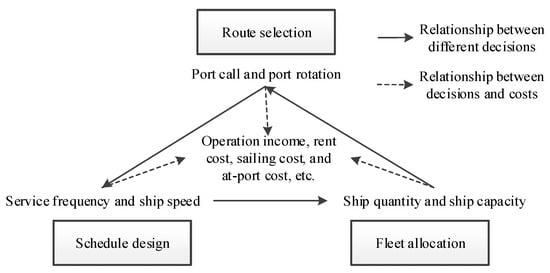
Figure 3.
Relationship between three subproblems.
Furthermore, all decisions directly affect the operation income and cost to varying degrees. For example, the container transport time will be longer with the increase in the number of port calls, leading to a lower transportation demand and less operation income. However, the ship capacity will expand with the increase in the number of port calls, thus generating the economy of scale and less operation cost. In addition, the round-trip time of ships is extended with the increase in number of port calls, and this may make the service schedule dissatisfy the schedule interval and arrival-time window of the trunk liner. Thus, we have to weigh the income and cost at the same time, which can be evaluated as follows.
The rent cost of ships, , depends on the ship quantity, ship capacity, and daily ship rent, and it can be calculated by using Formula (23). The at-port cost of ships, , depends on the port charge and container handling fee, and it can be calculated by using Formula (24). The sailing cost of ships, , depends on the sailing mileage, ship speed, and fuel-consumption rate, and it can be calculated by using Formula (25). The carbon-emission cost of ships, , depends on the fuel consumption when sailing at sea and working at port, and it can be calculated by using Formula (26). The multimodal transport subsidy, , depends on the container transportation demand attracted by the feeder liner, and it can be calculated by using Formula (27). The weekly operation cost, , can be calculated by using Formula (28), where the rent cost, at-port cost, sailing cost, and carbon emission cost of ships are added, and the multimodal transport subsidy of the feeder liner is subtracted. The weekly operation income, , can be calculated by using Formula (29), according to the transportation demand and freight rate. The weekly operation revenue of the feeder shipping network, , can be calculated by using Formula (30), and it needs to subtract the operation cost from the operation income of each feeder route.
4. Model Formulation
4.1. Assumptions
Referring to the studies on feeder shipping network optimization and shippers’ selection behavior analysis [6,8,32], the following assumptions are presented.
(i) The set of multimodal transport paths, namely the road path, rail path, and sea route, on each transport path is given.
(ii) The set of feeder routes, namely the port calls, port rotation, service frequency, and the sailing mileage, on each route is given.
(iii) The set of feeder ships, namely the container capacity and fuel-consumption rate of each ship, is known.
(iv) The feeder liner carries the transportation demand for foreign trade between the trunk port and feeder port, but it cannot carry the transportation demand for domestic trade between several feeder ports.
(v) The shippers are rational, as they always select the multimodal transport carrier and path with higher utility value.
(vi) The utility coefficients of shippers for brand effect, transport time, and freight rate are known.
4.2. Mathematical Model
Here, a mathematical model for the integrated planning of route selection, schedule design, and fleet allocation is developed, with the objective function of maximizing the weekly operation revenue of liner shipping network. The constraint conditions include the ship capacity limit, the speed-adjustment interval, the schedule interval, and the arrival-time window of the trunk liner. Moreover, the decision variables are the port calls, the port rotation, the service frequency, the ship speed, the ship capacity, and the ship quantity.
In the model, a nested Logit model is introduced to analyze the multimodal transport-path selection, taking into account shippers’ inertia preference for brand effect and non-inertia preference for transport time and freight rate. In addition, the analysis of the port-to-port shipping route is extended to the selection of the door-to-door transport path by introducing the road distance and unit freight rate, the railway transit period and base price, the freight rate of the trunk liner and feeder liner, and the committed transport time of the trunk liner.
The integrated optimization model is difficult to formulate and solve, as it contains multiple interrelated decision variables compared to the problem with one decision variable [2].
The ship speed is a continuous decision variable, and both the route selection and fleet allocation are binary decision variables. In addition, the sailing-time function, fuel-consumption function, arrival-time window, and nested Logit model are nonlinear functions. Thus, our model is a mixed-integer nonlinear programming formulation, which is shown as follows.
The constraints are as follows: Formulas (1)–(10) and
Objective Function (31) of our model is for maximizing the weekly operation revenue of the whole feeder shipping network. Formulas (1)–(10) utilize the nested Logit model for allocating the import and export demands to the multimodal transport paths. Formula (32) requires each feeder port to be served by only one feeder route. Formula (33) calculates the container volume when ships leave the trunk port. Formula (34) calculates the container volume when ships leave each feeder port. Formula (35) calculates the maximum container volume of ships according to the full load limit. Formula (36) requires that the maximum container volume does not exceed the capacity of the feeder ship. Formula (37) calculates the total at-port time of the ships on each feeder route. Formula (38) calculates the total sailing time of the ships on each feeder route. Formula (39) requires that the speed-adjustment interval be satisfied by the ship speed on each feeder route. Formula (40) calculates the round-trip time of ships on each feeder route. Formula (41) requires that the round-trip time of ships on each feeder route not exceed the schedule interval of the trunk liner. Formula (42) requires that the arrival time of each round trip satisfies the arrival-time window at the trunk port. Formula (43) calculates the ship quantity required according to the service frequency and round-trip time and requires the ship quantity required is to be less than the ship quantity allocated. Formula (44) calculates the ship quantity allocated to each feeder route. Formula (45) requires that each feeder ship be allocated only to one feeder route. Formula (46) calculates the rent cost of ships on each feeder route. Formula (47) calculates the at-port cost of the ships on each feeder route. Formula (48) calculates the sailing cost of the ships on each feeder route. Formula (49) calculates the carbon-emission cost of the ships on each feeder route. Formula (50) calculates the subsidy for container multimodal transport. Formula (51) calculates the weekly operation cost on each feeder route. Formula (52) calculates the weekly operation income on each feeder route. Formula (53) defines the binary decision variables of route selection and fleet allocation.
5. Algorithm Design
To solve the route-selection model with the nonlinear functions of sailing time and fuel consumption, the common method is to first linearize the nonlinear functions and then use CPLEX to solve the linear model [12,25,32,47]. However, there is currently no effective method to linearize the nested Logit model used in this study. Thus, we propose a particle swarm algorithm (PSO) framework embedded with the CPLEX solver by referring to the related literature [2,7,8,30,48]. In the framework, the PSO algorithm is used to handle the nonlinear nested Logit model, and CPLEX solves the linearized model after relaxing the nested Logit model.
The algorithm flowchart is shown in Figure 4, where the left side is the PSO algorithm, and the right side shows the process of the CPLEX solver. The PSO algorithm consists of the particle swarm construction, the fitness evaluation, and the particle-position update. In the PSO algorithm, particle swarm construction encodes the path-selection ratio from the nested logit model into the particle positions, and the particle-position update is used to improve the path-selection ratio. The particle fitness is evaluated based on the result of the CPLEX solver. For the process of the CPLEX solver, we first relax the nested Logit model and linearize the fuel-consumption function, operation-cost function, and arrival-time window in the relaxed model. Then, the proposed nonlinear programming model can be transformed into a linear formulation, which can be solved by CPLEX.
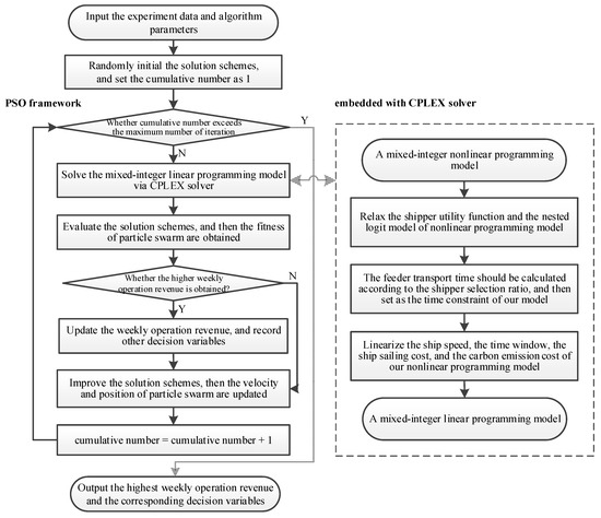
Figure 4.
Algorithm flowchart.
5.1. Model Relaxation and Linearization
To facilitate the model linearization, we relaxed the analysis on multimodal transport-path selection. In the relaxed model, the shippers’ path-selection ratios, , determined by Formulas (1)–(10) are regarded as known parameters. Then, the waterway transport time, , between trunk port and feeder ports can be inferred. Furthermore, the waterway transport time, , can be set as new time constraints, shown as Formulas (54) and (55).
The relaxed model is still a mix-integer nonlinear programming model, but it can be linearized completely [8,27,46,47,49]. The linearization process is as follows:
(i) For the nonlinear function in Formula (38), it can be linearized via Formulas (57) and (58) by establishing that . In addition, by substituting into Formulas (54) and (55), the linearized constraints of waterway transport time can be obtained via Formulas (59) and (60).
(ii) For the nonlinear arrival-time window, , in Formula (42), it should be transformed into , representing that there are sets of earliest arrival time and latest arrival time in the arrival-time window. We set as the binary decision variable of the arrival-time window, which is equal to 1 when the time window on feeder route is selected; otherwise, it is equal to 0. Then, the constraint of arrival-time window can be linearized via Formulas (61)–(64), where is an infinite positive number. Formula (61) requires that the arrival time of each round trip is not earlier than the earliest arrival time, and Formula (62) requires that the arrival time of each round trip is not later than the latest arrival time. Formula (63) restricts the cumulative number of the arrival-time window selected, and Formula (64) defines the binary decision variable of the arrival-time window selected.
(iii) To deal with the sailing cost, , and carbon emission cost, , of ships, we need to linearize the nonlinear function, . This nonlinear function can be expressed as by introducing the functions of and . Then, the unique nonlinear function, , can be linearized by referring to [31,47]. In the linearization process, we find the most approximate value, , of variable and then estimate the nonlinear function, , based on the tangent slope, . Formula (65) defines the value range of variable , and Formula (66) describes the approximation condition of variable . Because was obtained according to the tangent slope, we can use Formulas (67) and (68) to estimate the sailing cost and carbon emission cost of ships.
After the relaxation and linearization processes, the mixed-integer nonlinear programming model is transformed as a mixed-integer linear formulation, as follows.
The constraints are as follows: Formulas (32)–(37), (40), (41), (43)–(47) and (50)–(53).
5.2. Particle Swarm Optimization Framework
Here, we deal with the shippers’ multimodal transport-path selection. The PSO algorithm (Algorithm 1) based on heuristic rules is used to determine two interacting variables, i.e., the waterway transport time, , and the path-selection ratio, . In the PSO framework, we set and as the position and velocity of the th particle in the th iteration, respectively. Moreover, we set as the fitness of the th particle, as the historical optimal fitness of the th particle, and as the historical optimal fitness of the particle swarm. The main steps of the PSO framework are shown below.
| Algorithm 1: The proposed PSO framework |
|
Next, we explain some key aspects of the PSO procedure, including (i) particle swarm construction, (ii) particle fitness evaluation, and (iii) particle position update, as follows.
- (i)
- Particle swarm construction
Based on the multimodal transport network in Figure 1, we give an example of particle swarm in Figure 5, where P1-P9 denotes nine multimodal transport paths, and the symbols ‘−’ and ‘+’ denote the import and export direction, respectively. The path-selection ratios of P1 and P2 are 45% and 55% in the import direction, and they are 50% and 50% in the export direction. The path-selection ratios of P7, P8, and P9 are 20%, 35%, and 45% in the import direction, and the sum of three selection ratios is 100%. In fact, the path-selection ratios, , are usually generated randomly in the range of (0%, 100%) when initializing the particle swarm. To guarantee the uniformity and diversity of the particle swarm, we generate the of the initial particle swarm in the low (0%, 30%), medium (30%, 70%), and high (70%, 100%) ranges.
Figure 5.
Example of solution coding for the PSO algorithm.
- (ii)
- Particle fitness evaluation
Before evaluating the particle fitness, the import and export demands can be calculated according to the path-selection ratios, , in each particle, and these demands need to be aggregated to each feeder port. Then, the waterway transport time, , between the trunk port and feeder port can be inferred, and this transport time is used as the time constraints of the relaxed model.
After obtaining the transportation demand and waterway transport time, our mixed-integer linear programming model can be effectively solved based on the CPLEX solver. To avoid the failure of model solving, we first judge whether the waterway transport time, , is within a reasonable range. A poor fitness is given to the particle if the is unacceptable.
- (iii)
- Particle position update
According to the historical optimal position of each particle, , and the historical optimal position of the particle swarm, , we can update the position and velocity of the th particle based on Formulas (69) and (70). In the formulas, are the random numbers in the range of [0, 1], is the inertia factor of each particle moving at its original velocity, and are the learning factors of each particle moving to the historical optimal position.
The updated velocity of each particle should be within a certain range in order to avoid an excessive step size, but this range may not be fixed. We maintain a larger range in the early stage of iteration to help the particle swarm move to the optimal position quickly. In the later stage of iteration, we can utilize a smaller range to avoid deviating from the optimal position due to an excessive step size.
6. Computational Experiments
The computational experiments are conducted based on the multimodal transport system in Northern China, and the background and data of experiments are introduced in Section 6.1. In Section 6.2, we discuss our design of the comparative experiments of the enumeration method, the PSO framework embedded with CPLEX, and the general PSO algorithm to verify the effectiveness of our algorithm. To verify the feasibility and effectiveness of our model, we compare the results with or without the integrated optimization and the shipper selection behavior, respectively, in Section 6.3. We perform a sensitivity analysis on the operation parameters and the utility coefficients in Section 6.4. The PSO framework embedded with the CPLEX solver is encoded using MATLAB on the computer with Windows 10, 2.50 GHz, and 8G RAM. Referring to Eberhart and Shi [50] and Hu and Eberhart [51], the size of particle swarm is selected from the interval [20, 40], and the range of parameters in the PSO algorithm are and . Based on the known parameter ranges, we conduct multiple experiments with different parameter values. A set of parameters with the high convergence and the best fitness are set as the algorithm parameters, namely the size of the particle swarm is 30; the number of iterations is 200; and .
6.1. Experiments Parameters
6.1.1. Multimodal Transport Path
The inland transport demands from the provinces of Northern China need to gather at Dalian port or Qingdao port by means of the road transport, rail transport, and water transport. These demands are then transported to the overseas ports in Canada and the west coast of the United States via the trunk liner shipping established by the Dalian port or Qingdao port. The multimodal transport paths are shown in Figure 6, where the inland origins include Haerbin city in Heilongjiang province, Chifeng city in Neimenggu province, Huhehaote city in Neimenggu province, and Taiyuan city in Shanxi province. All ports of the feeder shipping network of Bohai Bay are shown in the right bottom of Figure 6, where the Dalian port is regarded as the trunk port. In Figure 6, the two multimodal transport paths from west to east in Haerbin are by rail transport to Dalian port and the road transport to Dandong port, respectively. The two multimodal transport paths from north to south in Chifeng are by rail transport to Dalian port and the road transport to Qinhuangdao port, respectively. The two multimodal transport paths from north to south in Huhehaote are by road–rail transport to Jingtang port and the road transport to Qingdao port, respectively. The two multimodal transport paths from north to south in Taiyuan are by rail transport to Huanghua port and the road transport to Qingdao port, respectively. For the feeder shipping network, the direct route of Huanghua–Dalian, the direct route of Dandong–Dalian, and the multi-port route of Qinhuangdao–Jingtang–Dalian can be established.
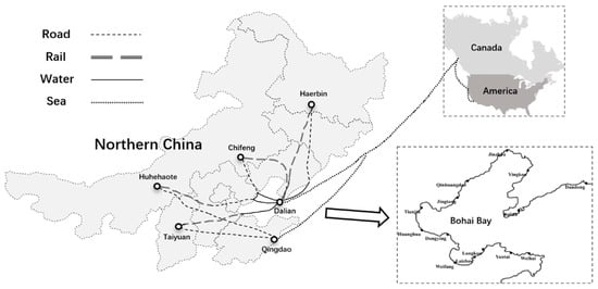
Figure 6.
Multimodal transport paths in Northern China.
6.1.2. Parameters of Multimodal Transport
The weekly import and export demands according to the survey data on the container freight are shown in Table 3. These import and export demands are not only from the cities themselves but also from the small-sized cities in the same province and the nearby cities in the adjacent provinces. We can obtain the route mileage, transport time, and freight rate from the 95,306 Railway Freight website, Jincheng Logistics website, and other websites. The transport mileage between the inland city and feeder port is shown in Table 4.
Table 3.
Weekly import and export demands.
Table 4.
Transport mileage between inland city and feeder port.
The freight rates of the trunk liner from Dalian port and Qingdao port to Vancouver port are, respectively, 5500 CNY/TEU and 6100 CNY/TEU, including the container handling fee, sea transport fee and freight transport insurance. The base price I of rail transport is 440 CNY/TEU, and the base price II of rail transport is 3.185 CNY/(TEU·km). The unit price of road transport is 5.73 CNY/(TEU·km), including the drivers fee, fuel fee, road fee, bridge fee, insurance fee, and depreciation fee.
The transshipment time is added to the transport time, the average speed of road transport is 70 km/h, and the committed transport time of the trunk liner is 25 days. The railway transit period generally consists of three parts, including 1 day for the shipment of cargo, 1 day for the transport time every 250 km, and 0 day for the special operation. Referring to the calibration results from the previous literature and the survey parameters of the freight market, the utility coefficients of shippers for transport time and freight rate in four inland origins are [650, 680, 670, 630] and [10,000, 9000, 12,000, 8700], respectively.
6.1.3. Parameters of Feeder Liner Shipping
To improve the multimodal transport demand and increase the weekly operation revenue, we conduct the integrated optimization for route, schedule, and fleet. The set of feeder routes is shown in Table 5, where the port calls, port rotation, service frequency, total sailing mileage of ships, and sailing mileage between two ports are included. The freight rate between the feeder port and trunk port is shown in Table 6, and this freight rate is related to the sailing mileage of direct routes. In addition to the multimodal transport demand, the import and export demands at each feeder port are shown in Table 6. The schedule interval of the trunk liner is 168 h, and the arrival-time window from Monday to Sunday is day/night, daytime, daytime, night, day/night, day/night, and day/night.
Table 5.
The set of feeder routes for the liner shipping network in Bohai Bay.
Table 6.
Freight rate, export demand, and import demand in Bohai Bay.
The set of feeder ships is , where there are three ships at 400 TEU, four ships at 650 TEU, three ships at 810 TEU, and four ships at 900 TEU. The full load limit of feeder ships is 90%, and the minimum and maximum ship speeds are 7 kn and 14 kn. The feeder ships are suitable for two shore bridges, so the container handling efficiency is generally 50 TEU per hour. The port charge of ships per trip is CNY 3000, and the container handling fee at each port is 15 CNY/TEU. The daily ship rent is 10.5 CNY/TEU, and the fuel-consumption cost is 2070 CNY/mt. The fuel-consumption rate of ships when sailing at sea is 0.012 mt, and the fuel-consumption rate of ships when working at port is 4 mt/day. The carbon-emission cost of fuel consumption is 157 CNY/t, and the subsidy for multimodal transport is 150 CNY/TEU.
6.2. Algorithm Validation
We propose the comparative experiments of the enumeration method, the PSO framework embedded with CPLEX (i.e., PSO framework), and the general PSO algorithm. For the programming model of the network design problem, it can be solved by using CPLEX for small-scale cases and the state-of-the-art branch and price method for large-scale cases. However, either CPLEX or branch and price method can only solve linear models, not our model, which cannot be linearized due to the existence of the Logit formulation. Currently, the common method for solving the nonlinearized model is heuristic. Thus, we choose to compare the proposed algorithm with the enumeration and the general PSO. The main steps of these two approaches are shown in Appendix A (Algorithms A1 and A2). The calculation time, maximum fitness (objective value), and average fitness of these three algorithms at different scales of instances are listed in Table 7. In this table, instance 4 × 13 × 7 denotes 4 multimodal transport paths, 13 feeder routes, and 7 feeder ships. The larger-scale instance means greater computational difficulty.
Table 7.
Effect comparison between enumeration method, PSO algorithm, and PSO framework.
The results in Table 7 show the following: (i) At the large-scale instance, the PSO framework and PSO algorithm can obtain satisfactory solutions within finite time, but the enumeration method calculates the objective value with significantly longer time. When the instance scale is larger than 8 × 25 × 7, the calculation time of the enumeration method has exceeded 259,200 s (three days). The enumeration method fails to obtain the objective value in finite time for larger-scale instances. Thus, the efficiency of the PSO framework and PSO algorithm can be verified. (ii) The maximum fitness and average fitness of the PSO framework are greater than those of the PSO algorithm at different scales of instances. When the instance scale is smaller than 8 × 25 × 7, the difference between the maximum fitness of the PSO framework and the objective value of the enumeration method is less than 1%. As we can see, the PSO framework embedded with the CPLEX solver is more advantageous in solving our integrated problem.
We further provide the maximum fitness curve and average fitness curve in the instance 8 × 25 × 14 of the PSO framework in Figure 7. With the increase in iteration number, the maximum fitness improves sharply and rapidly, from 4.65 × 10⁵ to 5.05 × 10⁵, and then it improves slightly to 5.13 × 10⁵. With the increase in the iteration number, the average fitness improves sharply and rapidly, from 0.81 × 10⁵ to 3.42 × 10⁵, and then it improves again slightly, to 3.75 × 10⁵. Figure 7 shows that the overall trend of the average fitness is rising. Moreover, the number of feasible solutions increases from 5 in the initial iteration to 30 in the final iteration. Therefore, the convergence and optimization abilities of our PSO framework embedded with CPLEX solver are verified.
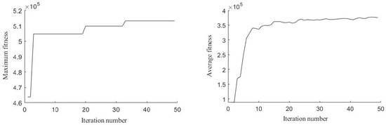
Figure 7.
Maximum fitness curve and average fitness curve of PSO framework.
6.3. Model Validation
We provide the results of the feeder network optimization to show the effectiveness of our model in Section 6.3.1. Then, the superiority of the integrated optimization is shown in Section 6.3.2. Then, Section 6.3.3 explores the impact of the shipper selection behavior.
6.3.1. Analysis on the Model Effectiveness
In the calculation results, there are 10 feeder routes and 10 feeder ships in the shipping network. The weekly operation income is 7.00 × 10⁵ CNY, the weekly operation cost is 1.87 × 10⁵ CNY, and the weekly operation revenue reaches 5.13 × 10⁵ CNY. Affected by the transport time and freight rate of rail transport, road transport and sea transport, the path-selection ratios of four multimodal transport paths related to the feeder shipping network have certain variation ranges. The path-selection ratios cannot exceed the variation range by using the integrated planning of route selection, schedule design, and fleet allocation. As for the multimodal transport paths related to the feeder shipping network, the average path-selection ratio is 32%, and the import and export demands are about 690 TEU. The port calls and port rotation of each feeder route are shown in Figure 8, and the service frequency, ship capacity, and ship speed of each feeder route are listed in Table 8.
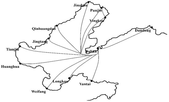
Figure 8.
Feeder liner shipping network in Bohai Bay.
Table 8.
Calculation results of feeder shipping network in Bohai Bay.
In Figure 8, we established the once-a-week multi-port route of Dalian–Yingkou–Panjin and established the twice-a-week direct routes for other feeder ports. As for these twice-a-week direct routes, the round-trip time of ships should be shorter than 84 h. However, due to the constraint of the arrival-time window, the round-trip time for the first trip should be within [48, 60]. In Table 8, the ship speed cannot exceed the speed-adjustment interval, and the round-trip time should satisfy the schedule interval and arrival-time window of the trunk liner. The liner shipping network covers all the 11 feeder ports, and the fleet allocation plan satisfies the given set of feeder ships. Since the feeder-transport demand is relatively small, three ships at 400 TEU and four ships at 650 TEU are selected. One ship at 810 TEU and two ships at 900 TEU are allocated to the feeder routes with a greater multimodal transport demand and the import and export demands. Because all of the constraints are satisfied, the feasibility of our model was verified.
6.3.2. Analysis on the Integrated Optimization
We conducted three experiments to analyze the necessity of the integrated planning of route selection (port call and port rotation), schedule design (service frequency and ship speed), and fleet allocation (ship capacity and ship quantity).
In Experiment (i), we only addressed the integrated planning of schedule design and fleet allocation in the liner shipping network composed of feeder routes numbered 1, 7, and 16–19. In the new results, the average service frequency of six feeder routes is twice a week, and the average ship capacity is added by 132 TEU. The weekly operation cost increased by 24%, the weekly operation revenue decreased by 11%, and path-selection ratio decreased by 5%. Clearly, this result is inferior to the result of the integrated planning.
In Experiment (ii), we addressed only the integrated planning of route selection and fleet allocation by increasing service frequencies in Table 5 by one. In the new results, we establish the twice-a-week multi-port routes of Dalian–Yingkou–Panjin, Dalian–Jiantang–Huanghua, and Dailian–Weifang–Longkou–Yantai and establish the three-a-week direct routes for other feeder ports due the schedule interval of the trunk liner. The path-selection ratio is increased by 6%, while the weekly operation cost is increased by 160%, and the weekly operation revenue decreases by 53%. On this basis, if the speed adjustment interval changed to [10, 11] kn, there are no differences in the schemes of the schedule design and fleet allocation. However, the path-selection ratio decreases by 9%, the weekly operation cost increases by 2%, and the weekly operation revenue decreases by 8%. Clearly, this result is inferior to the result of the integrated planning.
In Experiment (iii), we address only the integrated planning of route selection and schedule design based on all the feeder ships at 400 TEU. The path-selection ratio drops to nearly 0% in the new results because ships at 400 TEU cannot carry the multimodal transport demand. Due to the decrease in the multimodal transport income and subsidy, the weekly operation income decreases by 51%, and the weekly operation revenue decreases by 83%. In addition, we repeat the above experiment based on all the feeder ships at 900 TEU. The updated results show that the path-selection ratio is unchanged; however, the weekly operation cost increases by 88% due to higher rent cost, and the weekly operation revenue decreases by 34%. Clearly, this result is inferior to the result of the integrated planning.
According to the analysis of the results, the integrated optimization for route, schedule, and fleet contributes to improving the weekly operation revenue.
6.3.3. Analysis on the Shipper Selection Behavior
(i) Here, we analyze the impact of the shipper selection behavior for multimodal transport paths. Based on the import and export demands in Table 6, we first address the integrated optimization for route, schedule, and fleet without considering the multimodal transport-path selection. Then, we evaluate the shipper utility value of each multimodal transport path based on the service frequency and transport time of the whole feeder shipping network. Finally, we conduct the freight flow allocation according to the shipper utility value and update the weekly operation income and cost.
The new results establish the twice-a-week direct routes of Dandong and Tianjin and utilize the twice-a-week multi-port route of Dalian–Yingkou–Panjin–Jinzhou. In addition, the once-a-week multi-port routes of Dalian–Qinghuangdao–Jingtang–Huanghua and Dalian–Weifang–Longkou–Yantai should be established. Comparing the results with and without the shipper selection behavior, we find that there are no significant differences in the path-selection ratios and multimodal transport demands. However, the feeder ships that are allocated cannot carry all of the transport demands after the multimodal transport demand gathering at each feeder port. In addition, due to the increase in the container handling time of multimodal transport demand, the round-trip times on some feeder routes exceeded the schedule interval of the trunk liner. If we can enlarge the ship capacity and extend the schedule interval, the weekly operation cost increases significantly and the weekly operation revenue drops significantly.
(ii) Then, we further explore the impact of the unit freight rate on the shipper selection behavior. In the case with half of the unit freight rate of road transport, the new results show that the average freight rate of road and road–rail transport decreases by 14%, and the average path-selection ratios increase by 24%. The weekly operation income and cost, respectively, increase by 21% and 45%, so the weekly operation revenue just increases by 12%. In the case with a double unit freight rate of water transport, the new results show that the average freight rate of multimodal transport related to the feeder shipping network increases by 2% slightly, and there are nearly no differences in the path-selection ratios. The weekly operation income increases significantly by 128%, and the weekly operation revenue is still significantly improved, although the weekly operation cost increases by 26%.
The comparison results indicate that the consideration of multimodal transport-path selection contributes to improving the weekly operation revenue.
6.4. Sensitivity Analysis
Here, we conduct the sensitivity analysis on the operation parameters (i.e., the ship rent and the fuel price) and the utility coefficient of shippers’ preference.
6.4.1. Sensitivity Analysis on the Operation Parameters
We explore the impact of the ship rent and the fuel price [2,52]. Due to the constraint of arrival-time window, the current round-trip time for the first trip is set as [48, 60]. To improve the range for schedule design, we extend the arrival-time window to seven full days a week. Keeping other parameters of the above computational experiments unchanged, we recalculate the results of the feeder shipping network under different operation parameters, which are shown in Table 9. Related indicators under different operation parameters and are shown in Figure 9 and Figure 10, respectively.
Table 9.
Results of feeder shipping network under different time operation parameters.
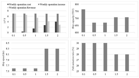
Figure 9.
Results under different daily rents, .
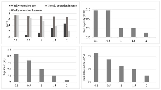
Figure 10.
Results under different fuel prices, .
(i) According to the results from the first five rows in Table 9 and Figure 9, we can find that with the gradual increase in the daily rent, , the liner shipping company should reduce the ship capacity or decrease the ship quantity to avoid a significant increase in the rent cost. However, the ship capacity cannot be reduced continuously to carry all of the transportation demand, so the liner shipping company changes the number of feeder routes from eight to seven to decrease the ship quantity. After that, the port calls have to increase with the decrease in the number of feeder routes, meaning that the container handling volume and time will be increased. In addition, the ship capacity is slightly increased, and the ship speed needs to improve to satisfy the schedule interval of the trunk liner. At this time, the increase in port calls will extend the transport time, so the path-selection ratio and the weekly operation income are reduced slightly. On this basis, due to the increase in operation cost, the weekly operation revenue is reduced significantly. It can be concluded that with the increase in daily rent, the liner shipping company tries to reduce the ship capacity allocated on the feeder route if the full load rate is relatively low, while the company should increase port calls for decreasing the number of routes and ships when the full load rate is relatively high.
(ii) According to the results from the last five rows in Table 9 and Figure 10, we can see that with the gradual increase in the fuel price, , the ship speed is reduced gradually, but it is always higher than the minimum speed. If the low speed cannot satisfy the arrival-time window or schedule interval of the trunk liner, the liner shipping company has to decrease the port calls or reduce the service frequency. However, since the sailing mileage of ships on one feeder route is relatively short, eight feeder routes can be maintained at the minimum speed. Moreover, the decrease in ship speed extends the transport time, which reduces the path-selection ratio and weekly operation income. The gradual increase in fuel-consumption cost leads to an increase in the weekly operation cost and a significant reduction in the weekly operation revenue. If the fuel price continues to rise, the ship speed is maintained at the minimum speed. At this time, the weekly operation cost is increased continuously, while the weekly operation revenue is reduced gradually. It can be concluded that with the increase in fuel price, the ship speed should be appropriately reduced in the speed-adjustment interval, which satisfies the arrival-time window and schedule interval of the trunk liner. If the time constraints are hardly satisfied by the low ship speed, the liner shipping company should reduce the service frequency or decrease the port calls. In this case, the weekly operation cost may be decreased, while the multimodal transport demand may be reduced.
6.4.2. Sensitivity Analysis on the Shippers’ Preference
As the transport carriers (i.e., brand effect) and freight rate are fixed, we analyze only the impact of the time utility coefficient, . A higher time utility coefficient implies that the shipper utility value is more sensitive to the multimodal transport time. Keeping other parameters unchanged, we list the results of the feeder shipping network under different time utility coefficients in Table 10. Related indicators under different time utility coefficients () are shown in Figure 11.
Table 10.
Results of feeder shipping network under different time utility coefficients.
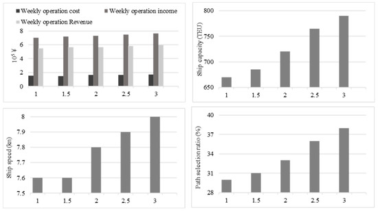
Figure 11.
Results under different time utility coefficient, .
(i) From the perspective of the operation income, the feeder routes 1/5/18 are selected under the 1.0× time utility coefficient. In this feeder shipping network, we establish one twice-a-week direct route for Dandong and Qinhuangdao and establish a once-a-week multi-port route for Dalian–Jiangtang–Huanghua. The short sailing mileage and high service frequency on the direct route reduce the container transport time, so the multimodal transport paths via Dandong and Qinhuangdao are time advantaged. With the increase in the time utility coefficient, the path-selection ratio and weekly operation income increase gradually. However, the time-advantaged multimodal transport paths were selected for the time-saving feeder routes, so we maintain the twice-a-week direct routes numbered 1/5. In addition, it is hard to improve the path-selection ratios by establishing a direct route for Jingtang and Huanghua, so we utilize the once-a-week multi-port route 18.
(ii) From the perspective of operation cost, with the gradual increase in multimodal transport demand, the ship capacities on each feeder route increase. As the container handling time increases, the liner shipping company has to improve the ship speed to satisfy the schedule interval constraint. At this time, the rent cost, at-port cost, sailing cost, and carbon emission cost of ships increase, but the weekly operation cost just improves a little due to the rise the in multimodal transport subsidy. In addition, the feeder transport time decreases with the increase in ship speed; then, the multimodal transport time reduces, and the path-selection ratio improves. However, because the waterway transport time has a small impact on the multimodal transport time, the increase in multimodal transport demand is limited. If the ship speed is improved continuously, the cost of fuel consumption increases significantly, leading to the increase in operation cost exceeding the increase in operation income. As we can see, there is no significant improvement in the ship speed with the increase in the time utility coefficient.
It can be concluded that when the shippers’ time utility coefficient is relatively high, it is wise to take advantage of the time advantage in multimodal transport paths by establishing direct routes to save sailing time or maintaining high service frequency to save at-port time. If the multimodal transport paths are cost-advantaged or the waterway transport time has a small impact on the multimodal transport time, the liner shipping company needs to weigh the increase in income and cost when using the measures of time-saving.
7. Conclusions
This study proposes a method for the integrated planning of feeder route selection, schedule design, and fleet allocation with shippers’ transport-path selection considered. We utilize the nested logit model to formulate the multimodal transport-path selection and then develop a mixed-integer nonlinear programming model for the integrated optimization for route, schedule, and fleet. To solve our model, a particle swarm optimization (PSO) framework embedded with CPLEX solver is proposed by combining the constraint relaxations and the linearization techniques with the heuristic rules. The computational experiments are conducted based on the multimodal transport system in Northern China to verify the effectiveness of our model and algorithm.
The application values and management insights are demonstrated as follows: (i) The proposed model is more consistent with the shipping practice, as we consider the speed adjustment interval, the ship capacity constraint, the arrival-time window, and the schedule interval of the trunk liner. Compared with the network design problem generated from scratch, it is more feasible and practical to carry out our route selection problem based on given schemes. Furthermore, the integrated optimization for route, schedule, and fleet makes it easier for planners to obtain global results. Our model can still be applied to address the case where the feeder routes or ships are given by adjusting the given schemes. Thus, our model can provide decision support for the operation practice and make the designed plan apply in practice with minimum revisions.
(ii) We utilize the nested logit model to analyze the multimodal transport-path selection, taking into account shippers’ inertia preference for brand effect and non-inertia preference for transport time and freight rate. This study extends the analysis of port-to-port shipping route to the selection of the door-to-door transport path by introducing the road distance and unit freight rate, the railway transit period and base price, the freight rate of the trunk liner and feeder liner, and the committed transport time of the trunk liner. Our research can not only provide the decision reference for the analysis of multimodal transport-path selection but can also help improve shipper satisfaction with multimodal transport and feeder liner service. Furthermore, our research is good to guide the shippers’ multimodal transport-path selection for raising the proportion of road–water transport and rail–water transport.
(iii) The sensitivity analyses of model parameters show that, with the increase in ship rent, feeder liner companies should reduce the ship capacity or increase the number of port calls. With the increase in fuel price, feeder liner companies should reduce the ship speed under the constraints of the arrival-time window and schedule interval. If shippers’ time utility coefficient is high, feeder liner companies should shorten the sailing time of ships by decreasing the number of port calls or shorten the at-port time of ships by increasing the service frequency. If the multimodal transport paths are cost-advantaged or the waterway transport time has a small impact on multimodal transport time, feeder liner companies need to weigh the increase in income and cost when using the measures of time-saving. These management insights can provide decision support for the operation practice of liner shipping network optimization.
There are some works we will investigate in the future: (i) Although green policies such as carbon emission cost and multimodal transport subsidy were taken into account, the calculation results do not significantly raise the proportion of road–water transport and rail–water transport with the objective of maximizing the weekly operation revenue of the feeder liner company. In the future, we will consider the multimodal transport-path selection objective of shippers, the operation revenue maximization objective of liner shipping companies, and the water transport proportion growth objective of transportation managers for promoting the development of low-carbon transportation. (ii) The International Maritime Organization requires that the sulfur content of fuel oil used by ships should not exceed 0.5% m/m after 1 January 2020, which greatly promotes the low-carbon process of water and sea transport. However, most liner shipping studies still focus on fuel-saving measures of ship speed reduction, and other green technologies, such as emission control areas, scrubbers, and shore power, should also be adopted. In the future, we will try to adopt the above green technologies by considering the carbon tax and subsidy policies.
Author Contributions
Methodology, L.G. and J.D.; Software, L.G.; Validation, N.H.; Investigation, J.Z.; Resources, J.D.; Writing—original draft, L.G. and J.D.; Writing—review & editing, J.Z. and N.H.; Supervision, J.Z.; Funding acquisition, J.D. All authors have read and agreed to the published version of the manuscript.
Funding
This work was supported by the Dalian Academy of Social Science (grant number 2022dlsky084) and the Dalian Federation of Social Science [grant number 2023dlskzd116].
Acknowledgments
The authors would like to thank the anonymous reviewers for their serious and rigorous comments.
Conflicts of Interest
The authors declare no conflict of interest.
Appendix A
Here, we show pseudocodes of the enumeration and general PSO used in Section 6.2.
| Algorithm A1: The general PSO |
|
| Algorithm A2: The enumeration method |
|
References
- Hellsten, E.O.; Sacramento, D.; Pisinger, D. A branch-and-price algorithm for solving the single-hub feeder network design problem. Eur. J. Oper. Res. 2022, 300, 902–916. [Google Scholar] [CrossRef]
- Wang, Y.D.; Wang, S.A. Deploying, scheduling, and sequencing heterogeneous vessels in a liner container shipping route. Transp. Res. Part E Logist. Transp. Rev. 2021, 151, 102365. [Google Scholar] [CrossRef]
- Santini, A.; Plum, C.E.M.; Ropke, S. A branch-and-price approach to the feeder network design problem. Eur. J. Oper. Res. 2018, 264, 607–622. [Google Scholar] [CrossRef]
- Msakni, M.K.; Fagerholt, K.; Meisel, F.; Lindstad, E. Analyzing different designs of liner shipping feeder networks: A case study. Transp. Res. Part E Logist. Transp. Rev. 2020, 134, 101839. [Google Scholar] [CrossRef]
- Bian, Y.Y.; Yan, W.; Hu, H.T.; Li, Z.Z. Feeder Scheduling and Container Transportation with the Factors of Draught and Bridge in the Yangtze River, China. J. Mar. Sci. Eng. 2021, 9, 964. [Google Scholar] [CrossRef]
- Jin, J.G.; Meng, Q.; Wang, H. Feeder vessel routing and transshipment coordination at a congested hub port. Transp. Res. Part B Methodol. 2021, 151, 1–21. [Google Scholar] [CrossRef]
- Zhen, L.; Wang, S.A.; Laporte, G.; Hu, Y. Integrated planning of ship deployment, service schedule and container routing. Comput. Oper. Res. 2019, 104, 304–318. [Google Scholar] [CrossRef]
- Du, J.; Wu, N.; Zhao, X.; Wang, J.; Guo, L.M. Container liner shipping schedule optimization with shipper selection behavior considered. Marit. Policy Manag. 2023, 1–25. [Google Scholar] [CrossRef]
- Tu, N.W.; Adiputrantob, D.; Fu, X.W.; Li, Z.C. Shipping network design in a growth market: The case of Indonesia. Transp. Res. Part E Logist. Transp. Rev. 2018, 117, 108–125. [Google Scholar] [CrossRef]
- Cheng, Q.; Wang, C.X. Container liner shipping network design with shipper’s dual preference. Comput. Oper. Res. 2021, 128, 105187. [Google Scholar] [CrossRef]
- Polat, O.; Günther, H.O.; Kulak, O. The feeder network design problem: Application to container services in the Black Sea region. Marit. Econ. Logist. 2014, 16, 343–369. [Google Scholar] [CrossRef]
- Zheng, J.F.; Yang, D. Hub-and-spoke network design for container shipping along the Yangtze River. J. Transp. Geogr. 2016, 55, 51–57. [Google Scholar] [CrossRef]
- Krile, S. Optimization approach in multi-stop routing of small islands. Sci. J. Marit. Univ. Szczec. 2018, 54, 9–16. [Google Scholar]
- Lin, Y.S.; Wang, X.F.; Hu, H.; Zhao, H. Research on feeder network design: A case study of feeder service for the port of Kotka. Eur. Transp. Res. Rev. 2020, 12, 61. [Google Scholar] [CrossRef]
- Paolo, F.; Gianfranco, F.; Simona, M.; Claudia, P.; Patrizia, S. Design and optimisation of an innovative two-hub-and-spoke network for the Mediterranean short-sea-shipping market. Comput. Ind. Eng. 2020, 149, 106847. [Google Scholar]
- Koza, D.F.; Desaulniers, G.; Ropke, S. Integrated Liner Shipping Network Design and Scheduling. Transp. Sci. 2020, 54, 512–533. [Google Scholar] [CrossRef]
- Hellsten, E.O.; Sacramento, D.; Pisinger, D. An adaptive large neighbourhood search heuristic for routing and scheduling feeder vessels in multi-terminal ports. Eur. J. Oper. Res. 2020, 287, 682–698. [Google Scholar] [CrossRef]
- Medić, D.; Krile, S.; Jelaska, I.; Bošnjak, R. Adriatic Sea Hub Ports Feeder Service Optimization Using Multi-Criteria Decision-Making Methods. Sustainability 2021, 13, 12325. [Google Scholar] [CrossRef]
- Zhu, S.Y.; Gao, J.J.; He, X.T.; Zhang, S.L.; Jin, Y.; Tan, Z.Y. Green logistics oriented tug scheduling for inland waterway logistics. Adv. Eng. Inform. 2021, 49, 101323. [Google Scholar] [CrossRef]
- Corey, J.; Wang, Q.; Zheng, J.F.; Sun, Y.L.; Du, H.M.; Zhu, Z.H. Container transshipment via a regional hub port: A case of the Caribbean Sea region. Ocean. Coast. Manag. 2022, 217, 105999. [Google Scholar] [CrossRef]
- Zhou, S.Q.; Ji, B.; Song, Y.L.; Yu, S.S.; Zhang, D.Z.; Woensel, T.V. Hub-and-spoke network design for container shipping in inland waterways. Expert Syst. Appl. 2023, 223, 119850. [Google Scholar] [CrossRef]
- Chen, K.; Yang, Z.Z.; Notteboom, T. The design of coastal shipping services subject to carbon emission reduction targets and state subsidy levels. Transp. Res. Part E Logist. Transp. Rev. 2014, 61, 192–211. [Google Scholar] [CrossRef]
- Wang, S.A.; Wang, H.; Meng, Q. Itinerary provision and pricing in container liner shipping revenue management. Transp. Res. Part E Logist. Transp. Rev. 2015, 77, 135–146. [Google Scholar] [CrossRef]
- Kashiha, M.; Thill, J.C.; Depken, C.A. Shipping route choice across geographies: Coastal vs. landlocked countries. Transp. Res. Part E Logist. Transp. Rev. 2016, 91, 1–14. [Google Scholar] [CrossRef]
- Yang, D.; Pan, K.; Wang, S.A. On service network improvement for shipping lines under the one belt one road initiative of China. Transp. Res. Part E Logist. Transp. Rev. 2018, 117, 82–95. [Google Scholar] [CrossRef]
- Duan, L.W.; Tavasszy, L.A.; Rezaei, J. Freight service network design with heterogeneous preferences for transport time and reliability. Transp. Res. Part E Logist. Transp. Rev. 2019, 124, 1–12. [Google Scholar] [CrossRef]
- Jiang, X.; Mao, H.J.; Wang, Y.D.; Zhang, H. Liner Shipping Schedule Design for Near-Sea Routes Considering Big Customers’ Preferences on Ship Arrival Time. Sustainability 2020, 12, 7828. [Google Scholar] [CrossRef]
- Chen, K.; Xu, S.H.; Haralambides, H. Determining hub port locations and feeder network designs: The case of China-West Africa trade. Transp. Policy 2020, 86, 9–22. [Google Scholar] [CrossRef]
- Zeng, Q.C.; Lu, T.Y.; Lin, K.C.; Yuen, K.F.; Li, K.X. The competitiveness of Arctic shipping over Suez Canal and China-Europe railway. Transp. Policy 2020, 86, 34–43. [Google Scholar] [CrossRef]
- Gao, S.Q.; Xin, X.; Li, C.; Liu, Y.R.; Chen, K. Container ocean shipping network design considering carbon tax and choice inertia of cargo owners. Ocean. Coast. Manag. 2022, 216, 105986. [Google Scholar] [CrossRef]
- Wang, H.; Meng, Q.; Zhang, X.N. Game-theoretical models for competition analysis in a new emerging liner container shipping market. Transp. Res. Part B Methodol. 2014, 70, 201–227. [Google Scholar] [CrossRef]
- Liu, Z.Y.; Meng, Q.; Wang, S.A.; Sun, Z. Global intermodal liner shipping network design. Transp. Res. Part E Logist. Transp. Rev. 2014, 61, 28–39. [Google Scholar] [CrossRef]
- Tran, N.K.; Haasis, H.D.; Buer, T. Container shipping route design incorporating the costs of shipping, inland/feeder transport, inventory and CO2 emission. Marit. Econ. Logist. 2016, 19, 667–694. [Google Scholar] [CrossRef]
- Su, X.M. A model of consumer inertia with applications to dynamic pricing. Prod. Oper. Manag. 2009, 18, 365–380. [Google Scholar] [CrossRef]
- Zhao, L.; Tian, P.; Li, X.Y. Dynamic pricing in the presence of consumer inertia. Omega 2012, 40, 137–148. [Google Scholar] [CrossRef]
- Bronnenberg, B.; Dubé, J.P. The Formation of Consumer Brand Preferences. Annu. Rev. Econ. 2017, 9, 353–382. [Google Scholar] [CrossRef]
- Mesa-Arango, R.; Ukkusuri, S.V. Attributes driving the selection of trucking services and the quantification of the shipper’s willingness to pay. Transp. Res. Part E Logist. Transp. Rev. 2014, 71, 142–158. [Google Scholar] [CrossRef]
- Jiang, X.D.; Fan, H.M.; Luo, M.F.; Xu, Z.L. Strategic port competition in multimodal network development considering shippers’ choice. Transp. Policy 2020, 90, 68–89. [Google Scholar] [CrossRef]
- Zhang, R.; Zhu, L.C. Threshold incorporating freight choice modeling for hinterland leg transportation chain of export containers. Transp. Res. Part A Policy Pract. 2019, 130, 858–872. [Google Scholar] [CrossRef]
- Zheng, J.F.; Meng, Q.; Sun, Z. Liner hub-and-spoke shipping network design. Transp. Res. Part E Logist. Transp. Rev. 2015, 75, 32–48. [Google Scholar] [CrossRef]
- Cariou, P.; Cariou, A.; Larbi, R.; Hamdan, S. Liner shipping network design with emission control areas: A genetic algorithm-based approach. Transp. Res. Part D Transp. Environ. 2018, 63, 604–621. [Google Scholar] [CrossRef]
- Zhou, J.M.; Zhao, Y.Z.; Niu, X.W. Two-Phase Optimization Models for Liner Shipping Network Based on Hub Ports Cooperation: From the Perspective of Supply-Side Reform in China. J. Adv. Transp. 2021, 2021, 6639218. [Google Scholar] [CrossRef]
- Zheng, J.F.; Gao, Z.Y.; Yang, D. Network Design and Capacity Exchange for Liner Alliances with Fixed and Variable Container Demands. Transp. Sci. 2015, 49, 886–899. [Google Scholar] [CrossRef]
- Akbar, A.; Aasen, A.K.A.; Msakni, M.K.; Fagerholt, K.; Lindstad, E.; Meisel, F. An economic analysis of introducing autonomous ships in a short-sea liner shipping network. Int. Trans. Oper. Res. 2021, 28, 1740–1764. [Google Scholar] [CrossRef]
- Xin, X.; Wang, X.L.; Ma, L.J.; Chen, K.; Ye, M.Y. Shipping network design–infrastructure investment joint optimization model: A case study of West Africa. Marit. Policy Manag. 2022, 49, 620–646. [Google Scholar] [CrossRef]
- Wang, S.A.; Alharbi, A.; Davy, P. Liner ship route schedule design with port time windows. Transp. Res. Part C Emerg. Technol. 2014, 41, 1–17. [Google Scholar] [CrossRef]
- Jiang, X.; Mao, H.J.; Zhang, H. Simultaneous optimization of the liner shipping route and ship schedule designs with time windows. Math. Probl. Eng. 2020, 2020, 3287973. [Google Scholar] [CrossRef]
- Liu, Y.; Xin, X.; Yang, Z.; Chen, K.; Li, C. Liner shipping network—Transaction mechanism joint design model considering carbon tax and liner alliance. Ocean. Coast. Manag. 2021, 212, 105817. [Google Scholar] [CrossRef]
- Zheng, J.F.; Hou, X.J.; Qi, J.W.; Yang, L.X. Liner ship scheduling with time-dependent port charges. Marit. Policy Manag. 2020, 49, 18–38. [Google Scholar] [CrossRef]
- Eberhart, R.; Shi, Y. Tracking and optimizing dynamic system with particle swarms. In Proceedings of the Congress on Evolutionary Computation, Seoul, Republic of Korea, 27–30 May 2001; pp. 94–97. [Google Scholar]
- Hu, X.; Eberhart, R. Multiobjective optimization using dynamic neighborhood particle swarm optimization. In Proceedings of the Congress on Evolutionary Computation, Honolulu, HI, USA, 12–17 May 2002; pp. 1677–1681. [Google Scholar]
- Lashgari, M.; Akbari, A.A.; Nasersarraf, S. A new model for simultaneously optimizing ship route, sailing speed, and fuel consumption in a shipping problem under different price scenarios. Appl. Ocean. Res. 2021, 113, 102725. [Google Scholar] [CrossRef]
Disclaimer/Publisher’s Note: The statements, opinions and data contained in all publications are solely those of the individual author(s) and contributor(s) and not of MDPI and/or the editor(s). MDPI and/or the editor(s) disclaim responsibility for any injury to people or property resulting from any ideas, methods, instructions or products referred to in the content. |
© 2023 by the authors. Licensee MDPI, Basel, Switzerland. This article is an open access article distributed under the terms and conditions of the Creative Commons Attribution (CC BY) license (https://creativecommons.org/licenses/by/4.0/).