
Numerical Simulation Study on Ship–Ship Interference in Formation Navigation in Full-Scale Brash Ice Channels


Abstract
:1. Introduction
2. Numerical Method
2.1. CFD–DEM Coupling
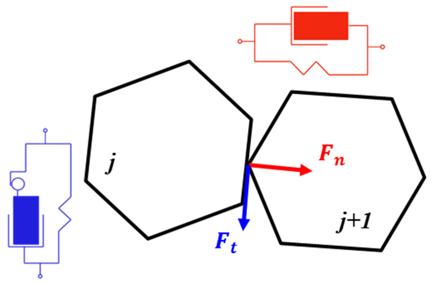
2.2. Particle Contact Model in the DEM
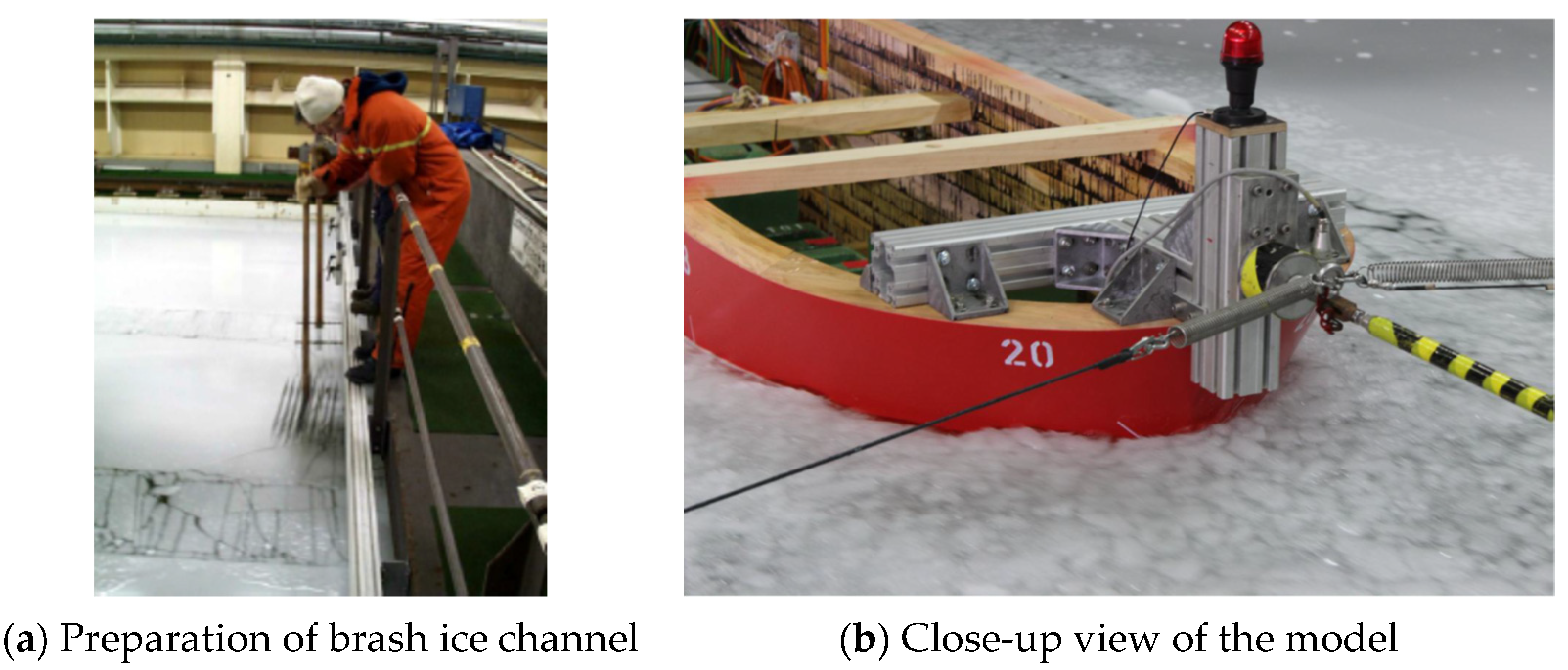
3. Ice Tank Test Description
4. Numerical Simulation
4.1. Ship Model
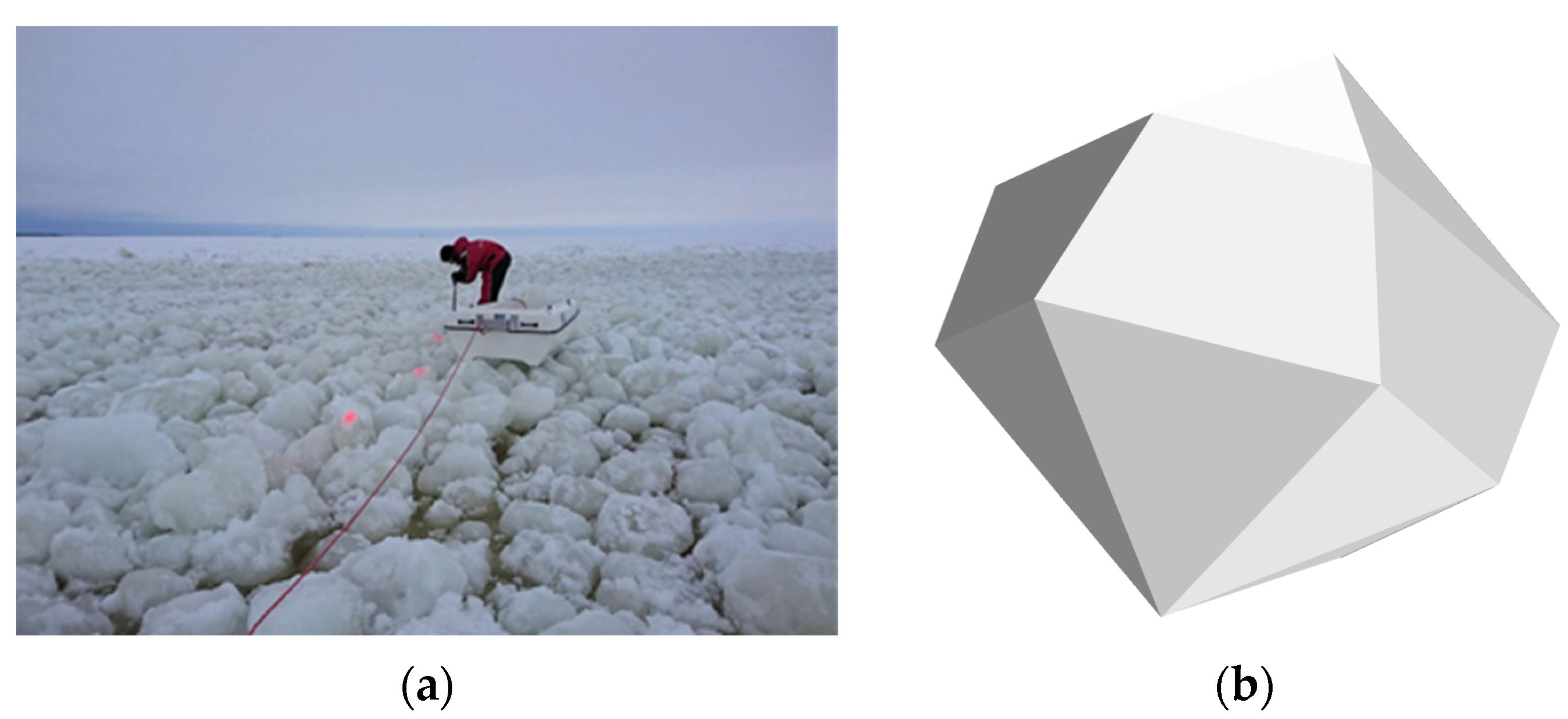
4.2. Brash Ice Model
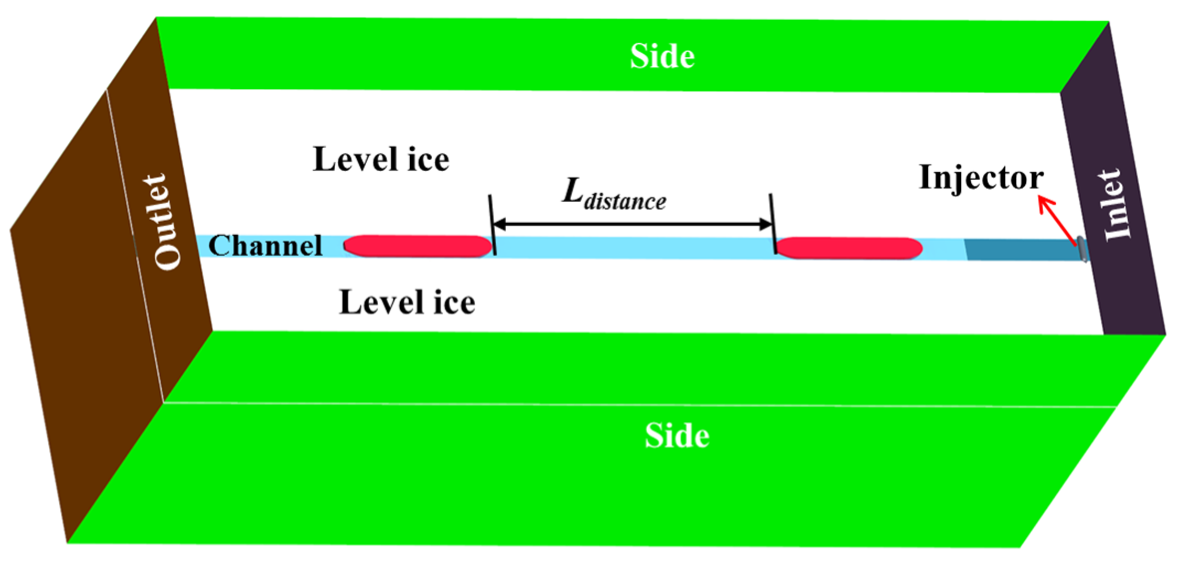
4.3. Computational Domain
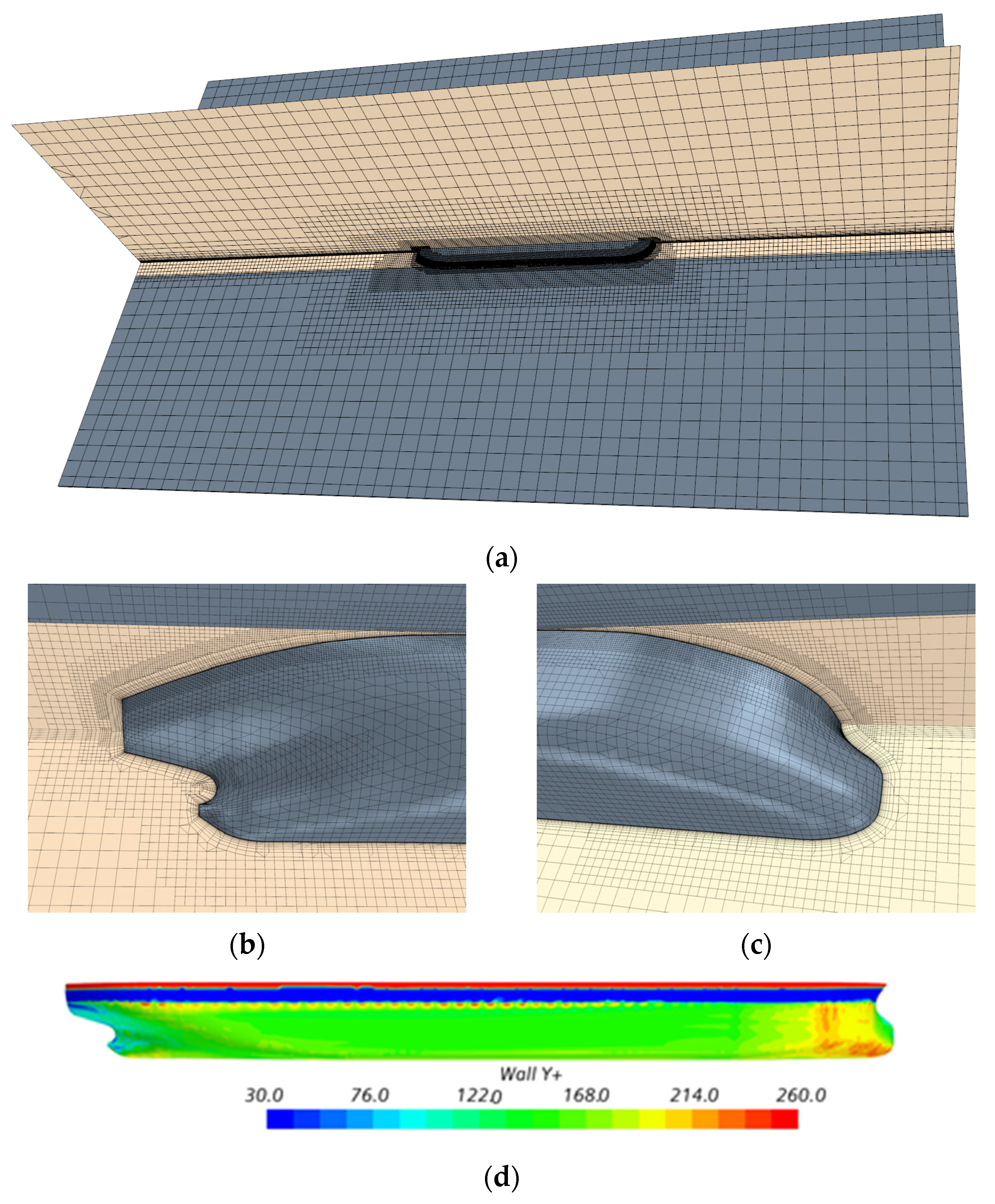
4.4. Grid Generation
5. Comparison between Simulation Results and Test Results
6. Analysis of Formation Navigation Simulation Results
6.1. Analysis of Simulation Results
6.2. Hydrodynamic Interaction between Ships
6.3. Ship–Ice Interaction and Ship–Ship Interference Phenomenon
7. Discussion
8. Conclusions
- (1)
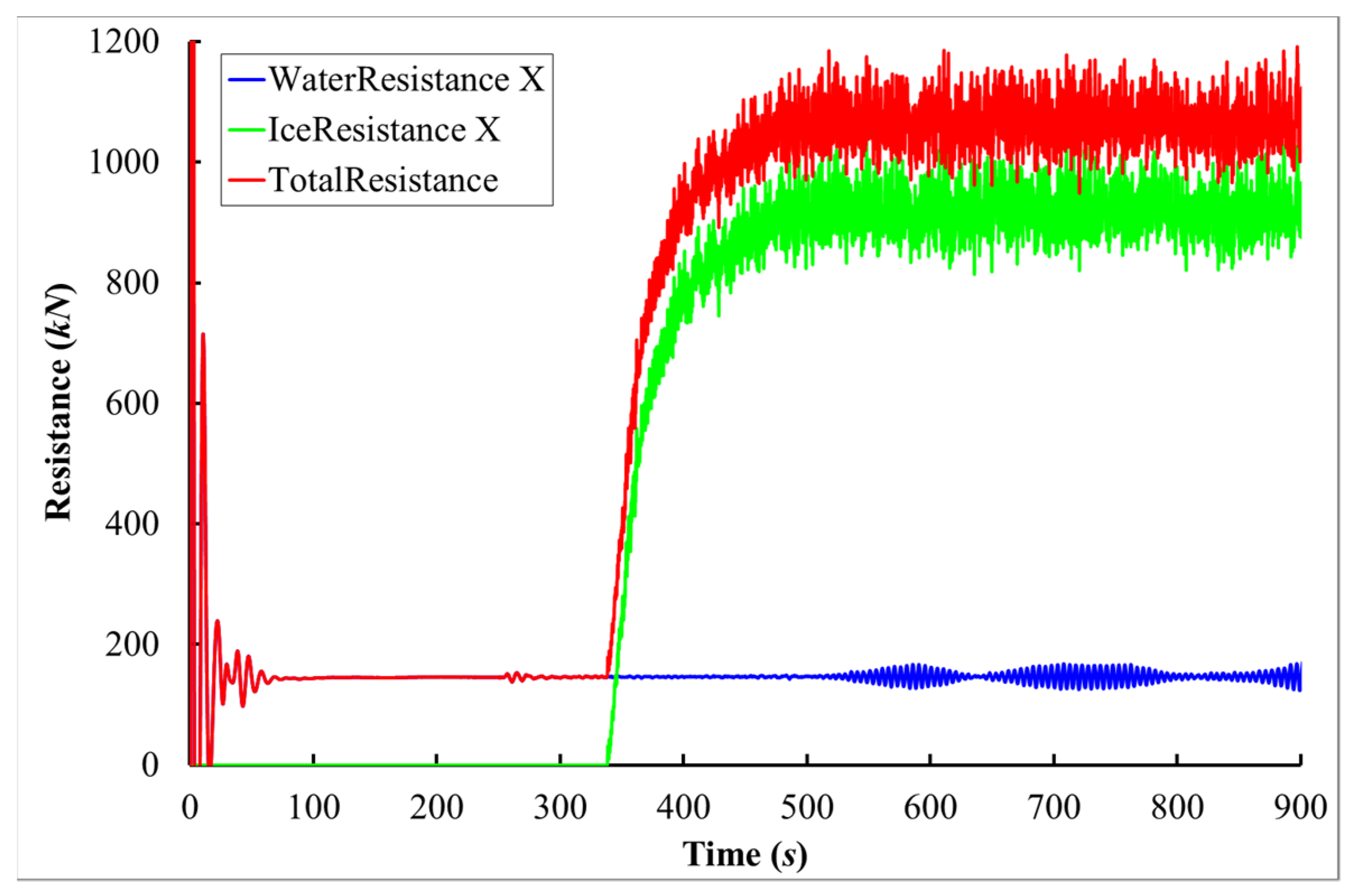
- The difference in total resistance between the full-scale simulation and the ice tank test is about 4%. The simulation results of the total resistance at full scale align well with the test results.
- (2)
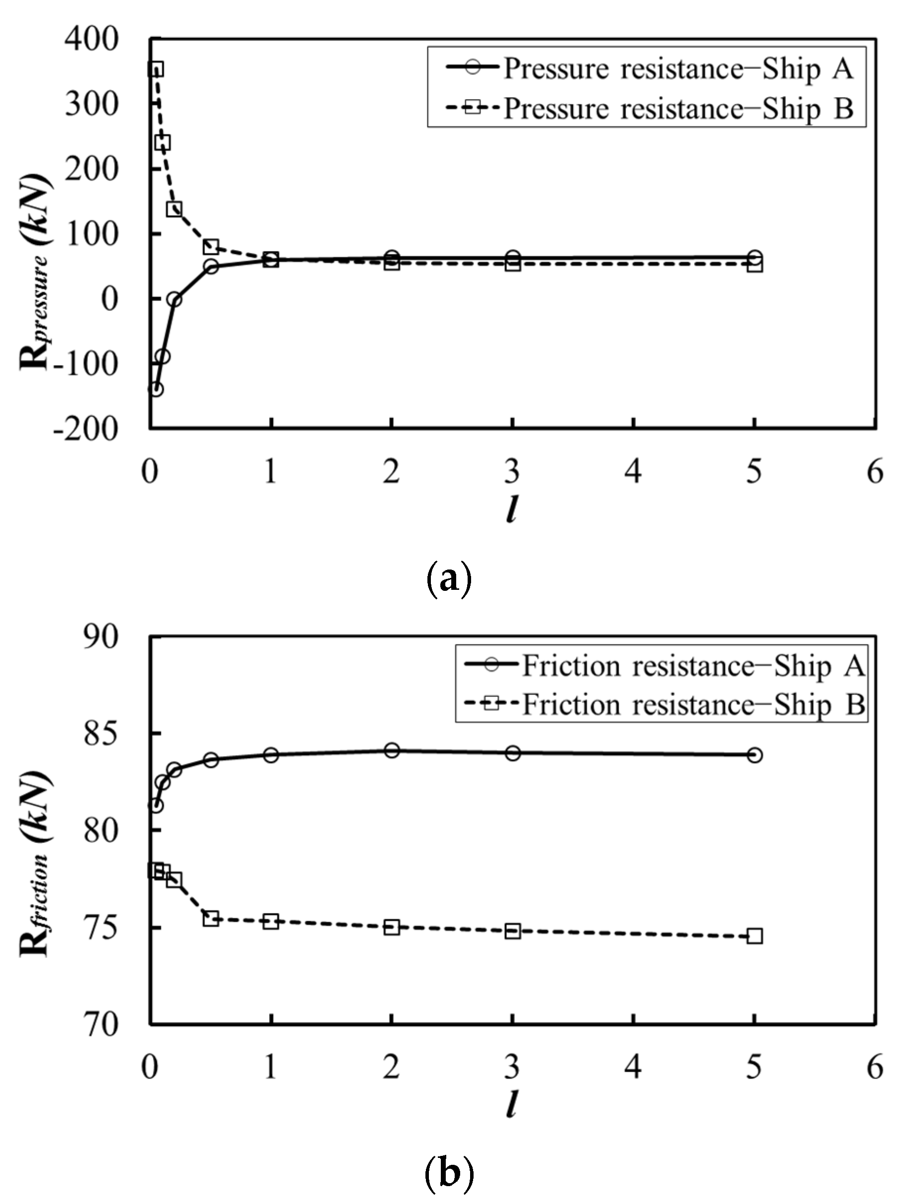
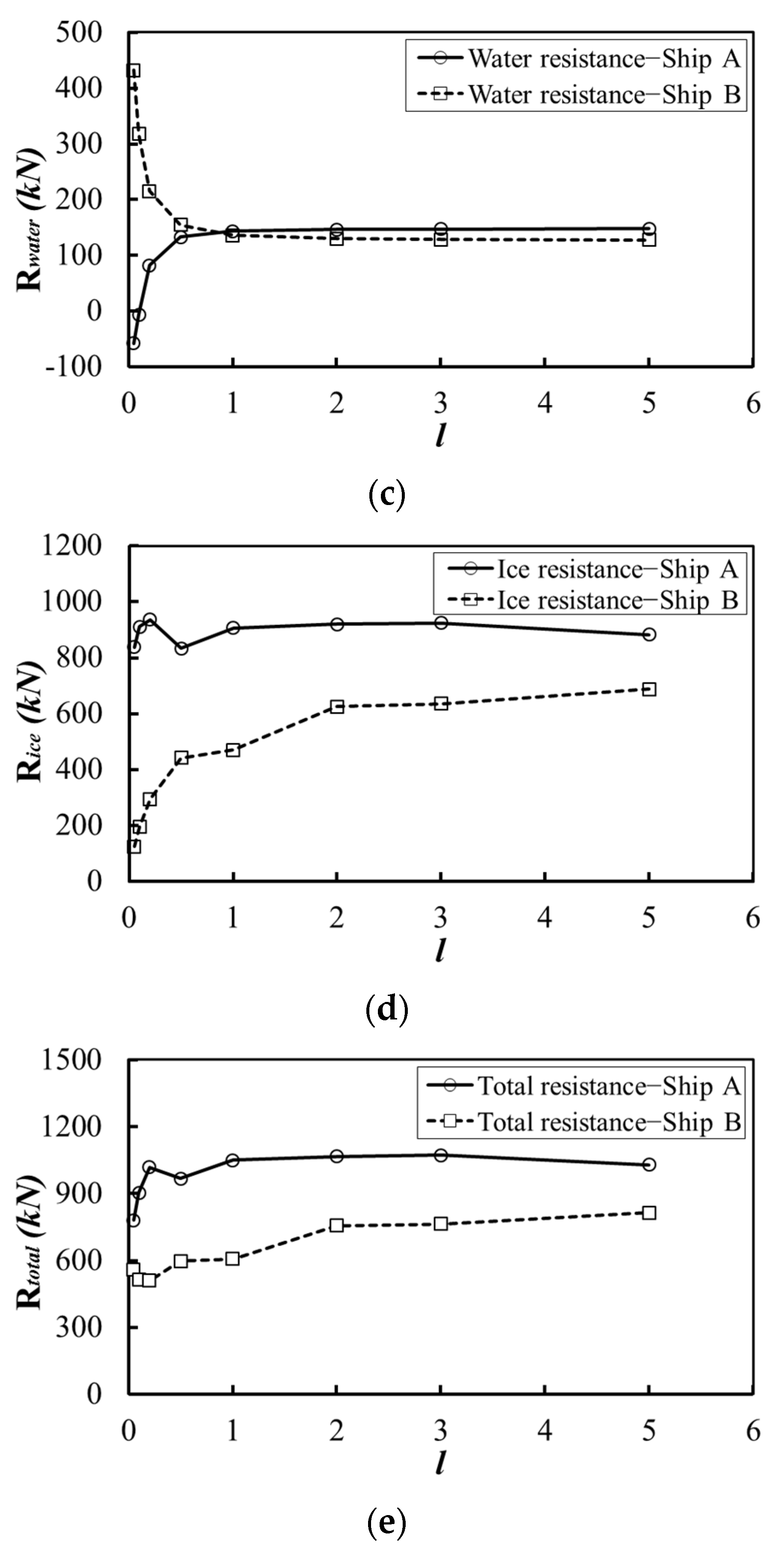
- The distance between ships during formation navigation has a significant impact on their resistance performance. When , as the distance decreases, the water resistance of Ship A increases, while that of Ship B decreases. When , the ice resistance of Ship A remains largely unaffected, whereas the ice resistance of Ship B decreases as the distance decreases. When , the total resistance of Ship B can be reduced by more than 25%.
- (3)
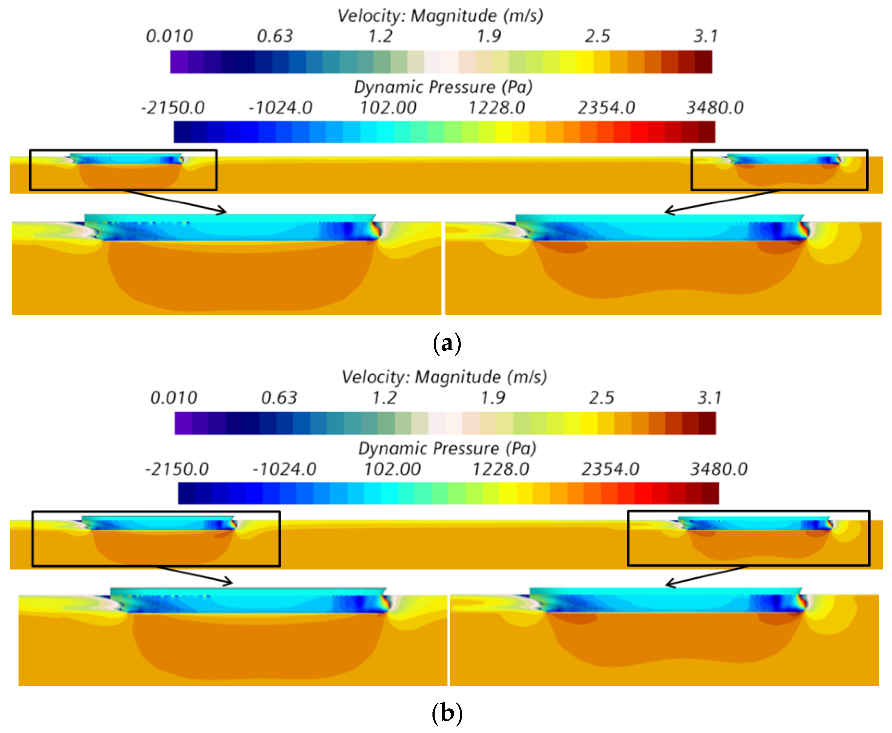
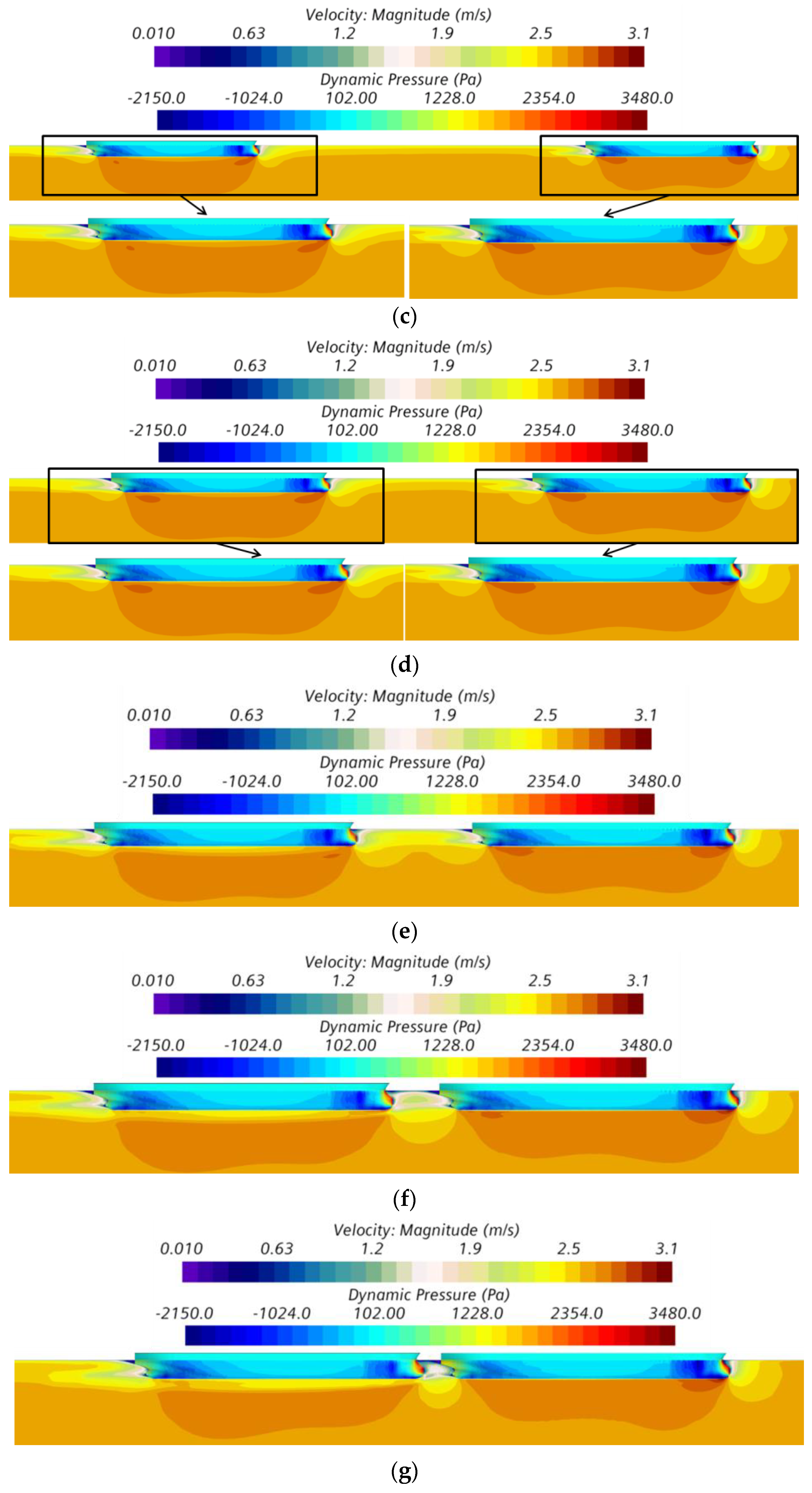
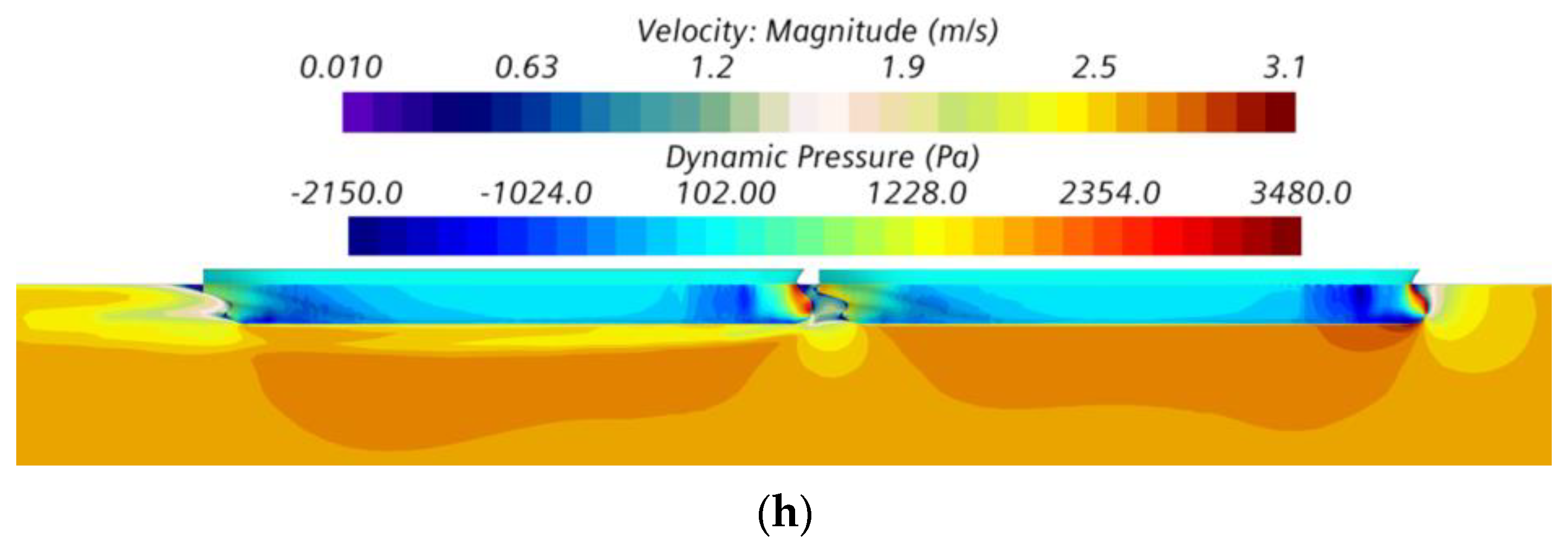
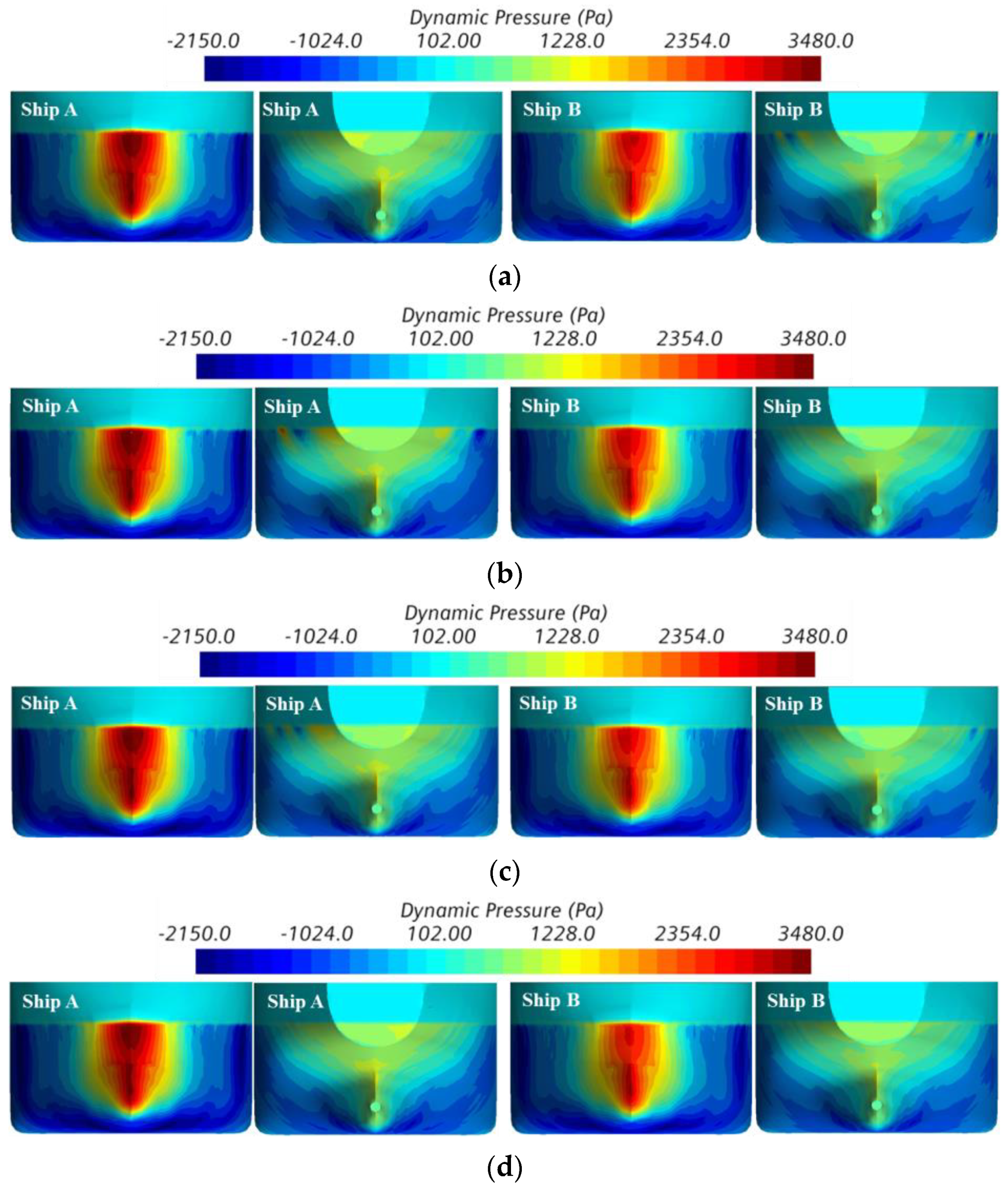
- The influence of distance on the velocity field between the two ships and the dynamic pressure distribution on the hull differs. When , the velocity field and dynamic pressure distribution on the hull are not significantly affected by distance. When , the effects become more pronounced.
- (4)
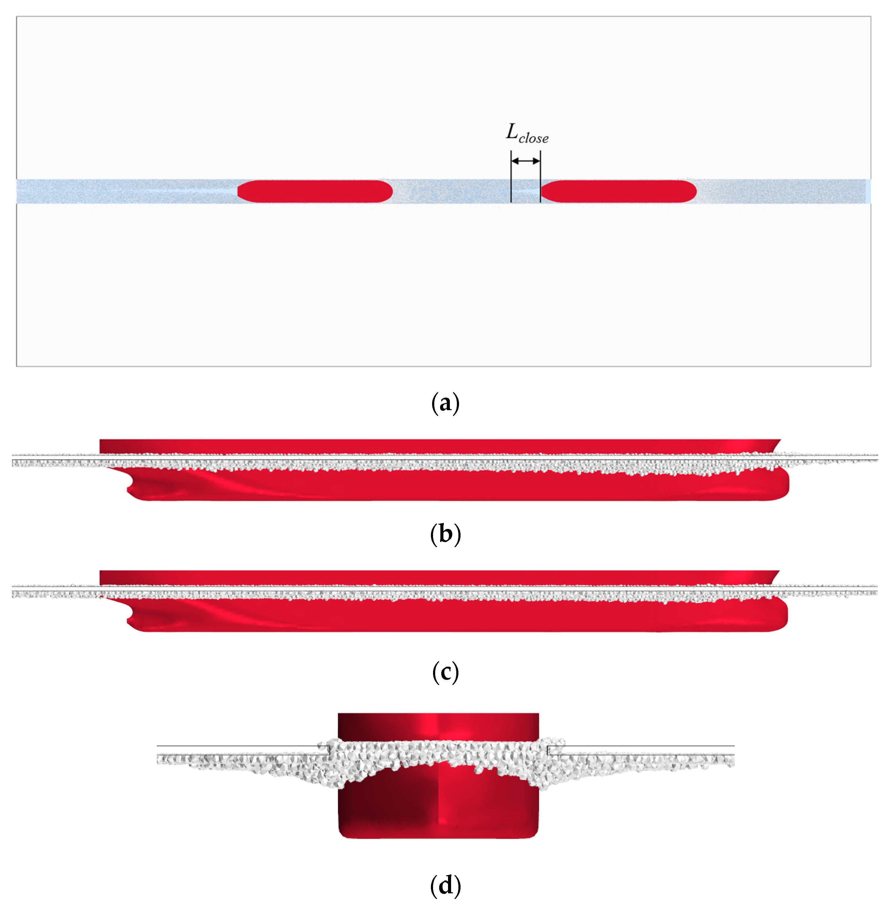
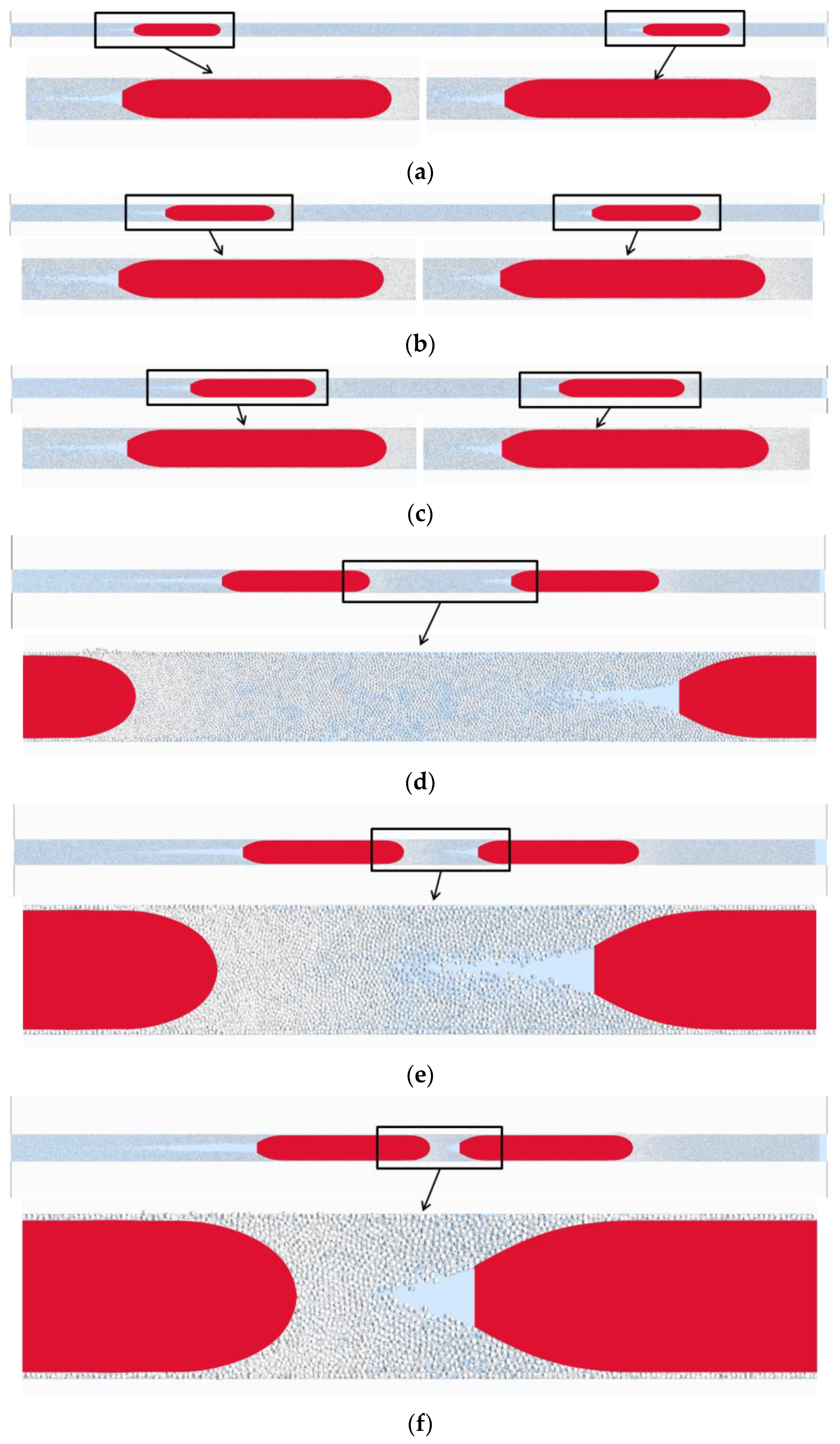
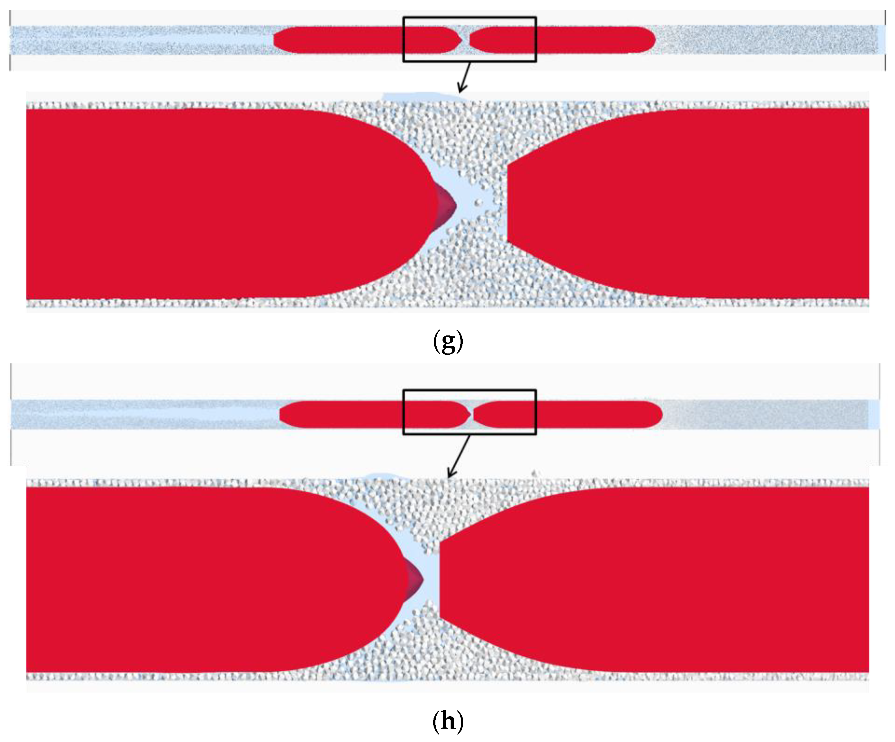
- Ship–ice interaction and ship–ship interference are greatly influenced by the distance between the ships. The length of the ice wake behind Ship B is longer than that behind Ship A, approximately equal to about 20% of Lpp. Notably, when , Ship A exhibits favorable interference with the ice accumulation of Ship B.
Author Contributions
Funding
Institutional Review Board Statement
Informed Consent Statement
Data Availability Statement
Conflicts of Interest
References
- Matala, R.; Suominen, M. Scaling principles for model testing in old brash ice channel. Cold Reg. Sci. Technol. 2023, 210, 103857. [Google Scholar] [CrossRef]
- Xie, C.; Zhou, L.; Ding, S.F.; Liu, R.W.; Zheng, S.J. Experimental and numerical investigation on self-propulsion performance of polar merchant ship in brash ice channel. Ocean Eng. 2023, 261, 113424. [Google Scholar] [CrossRef]
- Luo, W.Z.; Jiang, D.P.; Wu, T.C.; Guo, C.Y.; Wang, C.; Deng, R.; Dai, S.S. Numerical simulation of an ice-strengthened bulk carrier in brash ice channel. Ocean Eng. 2020, 196, 106830. [Google Scholar] [CrossRef]
- Guo, W.; Zhao, Q.S.; Tian, Y.K.; Zhang, C.W. Research on total resistance of ice-going ship for different floe ice distributions based on virtual mass method. Int. J. Nav. Arch. Ocean Eng. 2020, 12, 957–966. [Google Scholar] [CrossRef]
- Huang, L.F.; Tuhkuri, J.; Igrec, B.; Li, M.H.; Stagonas, D.; Toffoli, A.; Cardiff, P.; Thomas, G. Ship resistance when operating in floating ice floes: A combined CFD&DEM approach. Mar. Struct. 2020, 74, 102817. [Google Scholar]
- Xie, C.; Zhou, L.; Wu, T.C.; Liu, R.W.; Zheng, S.J.; Tsuprik, V.G.; Bekker, A. Resistance Performance of a Ship in Model-Scaled Brash Ice Fields Using CFD and DEM Coupling Model. Front. Energy Res. 2022, 10, 895948. [Google Scholar] [CrossRef]
- Matala, R.; Suominen, M. Investigation of vessel resistance in model scale brash ice channels and comparison to full scale tests. Cold Reg. Sci. Technol. 2022, 201, 103617. [Google Scholar] [CrossRef]
- Mucha, P. Fully-Coupled CFD-DEM for Simulations of Ships Advancing Through Brash Ice. In Proceedings of the SNAME Maritime Convention, Tacoma, DC, USA, 30 October–1 November 2019; Volume 1. [Google Scholar]
- Zhang, J.; Zhang, Y.; Shang, Y.; Jin, Q.; Zhang, L. CFD-DEM based full-scale ship-ice interaction research under FSICR ice condition in restricted brash ice channel. Cold Reg. Sci. Technol. 2022, 194, 103454. [Google Scholar] [CrossRef]
- Polojärvi, A.; Gong, H.Y.; Tuhkuri, J. Comparison of Full-Scale and DEM Simulation Data on Ice Loads Due to Floe Fields on a Ship Hull. In Proceedings of the 26th International Conference on Port and Ocean Engineering under Arctic Conditions, Moscow, Russia, 14–18 June 2021. [Google Scholar]
- Ferziger, J.; Peric, M.L. Computational Methods for Fluid Dynamics; Springer: Cham, Switzerland, 2001. [Google Scholar]
- Norouzi, H.R.; Zarghami, R.; Sotudeh-Gharebagh, R.; Mostoufi, N. Coupled CFD-DEM Modeling: Formulation, Implementation and Application to Multiphase Flows; John Wiley & Sons: Minneapolis, MN, USA, 2016. [Google Scholar]
- Siemens PLM Software, Simcenter STAR-CCMþ® Documentation; Siemens Digital Industries Software: Plano, TX, USA, 2019; Volume 1, 7482–7486.
- Cundall, P.A.; Strack, O.D. A Discrete Numerical Model for Granular Assemblies. Géotechnique 1979, 29, 47–65. [Google Scholar] [CrossRef]
- IO 509/12; Brash Ice Tests for a Panmax Bulker with Ice Class 1B. HSVA: Hamburg, Germany, 2013.
- ITTC. General Guidance and Introduction to Ice Model Test; ITTC Report: Hamburg, Germany, 2017. [Google Scholar]


| Principal Hull Data | Abbreviation | Full Scale | Model Scale |
|---|---|---|---|
| Scale | λ | 1 | 30.682 |
| Length between perpendiculars | Lpp (m) | 217.00 | 7.073 |
| Length at scantling draft | Lwl_Scantl. (m) | 221.07 | 7.205 |
| Length at ballast draft | Lwl_Ballast. (m) | 214.35 | 6.986 |
| Breadth molded at DWL | B (m) | 32.25 | 1.051 |
| Scantling draft | TFScantl. (m) | 14.73 | 0.480 |
| TAScantl. (m) | 14.73 | 0.480 | |
| Ballast draft | TFBallast (m) | 7.15 | 0.233 |
| TABallast (m) | 5.05 | 0.165 |
| Ice Class | Loading Condition | Ship Speed (Full Scale) (kn) | Ship Speed (Model Scale)(m/s) | Target Ice Thickness (Full Scale) (m) | Target Ice Thickness (Model Scale) (mm) |
|---|---|---|---|---|---|
| FSICR IA | Loaded draft | 5.0 | 0.464 | 1.42 | 46.3 |
| FSICR IA | Ballast draft | 5.0 | 0.464 | 1.42 | 46.3 |
| Parameter | Value |
|---|---|
| Elastic Modulus E (GPa) | 2.7 |
| Poisson’s ratio γ | 0.35 |
| Ice–ship friction coefficient f | 0.1 |
| Density ρi (kg/m3) | 920 |
| Brash ice diameter (m) | approx. 0.71 |
| Ice thickness (m) | 1.42 |
| /m | Resistance Value/kN | Percentage (%) | Error (%) | ||
|---|---|---|---|---|---|
| 1.42 | Experimental results (N) | Total resistance | 1075.2 | ---- | ---- |
| Simulation results (N) | Water resistance | 144.4 | 14.0 | ---- | |
| Brash ice resistance | 887.6 | 86.0 | ---- | ||
| Total resistance | 1032.1 | 100 | −4.01 |
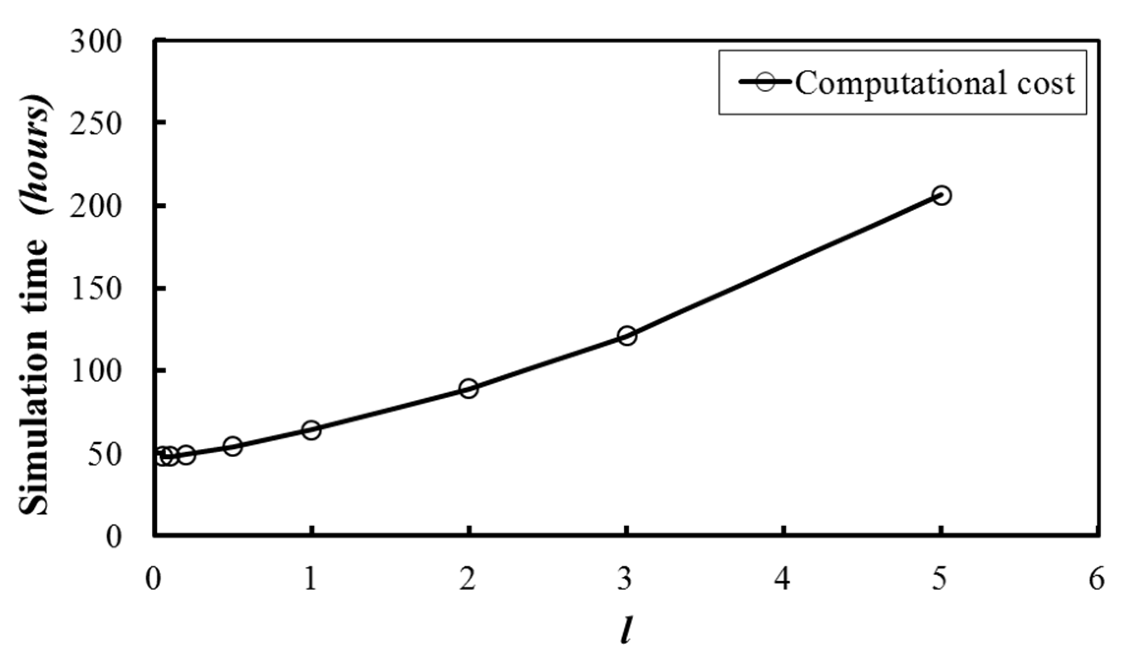
| Case 1 | Case 2 | Case 3 | Case 4 | Case 5 | Case 6 | Case 7 | Case 8 | |
|---|---|---|---|---|---|---|---|---|
| l | 0.05 | 0.1 | 0.2 | 0.5 | 1.0 | 2.0 | 3.0 | 5.0 |
| Case 1 | Case 2 | Case 3 | Case 4 | Case 5 | Case 6 | Case 7 | Case 8 | |
|---|---|---|---|---|---|---|---|---|
| l | 0.05 | 0.1 | 0.2 | 0.5 | 1.0 | 2.0 | 3.0 | 5.0 |
| Grid cell count (millions) | 235.6 | 235.6 | 236.6 | 238.6 | 241.7 | 246.2 | 251.0 | 257.6 |
| Simulation time (hours) | 48 | 48 | 49 | 54 | 64 | 89 | 121 | 206 |
Disclaimer/Publisher’s Note: The statements, opinions and data contained in all publications are solely those of the individual author(s) and contributor(s) and not of MDPI and/or the editor(s). MDPI and/or the editor(s) disclaim responsibility for any injury to people or property resulting from any ideas, methods, instructions or products referred to in the content. |
© 2023 by the authors. Licensee MDPI, Basel, Switzerland. This article is an open access article distributed under the terms and conditions of the Creative Commons Attribution (CC BY) license (https://creativecommons.org/licenses/by/4.0/).
Share and Cite
Xie, C.; Zhou, L.; Lu, M.; Ding, S.; Zhou, X. Numerical Simulation Study on Ship–Ship Interference in Formation Navigation in Full-Scale Brash Ice Channels. J. Mar. Sci. Eng. 2023, 11, 1376. https://doi.org/10.3390/jmse11071376
Xie C, Zhou L, Lu M, Ding S, Zhou X. Numerical Simulation Study on Ship–Ship Interference in Formation Navigation in Full-Scale Brash Ice Channels. Journal of Marine Science and Engineering. 2023; 11(7):1376. https://doi.org/10.3390/jmse11071376
Chicago/Turabian StyleXie, Chang, Li Zhou, Mingfeng Lu, Shifeng Ding, and Xu Zhou. 2023. "Numerical Simulation Study on Ship–Ship Interference in Formation Navigation in Full-Scale Brash Ice Channels" Journal of Marine Science and Engineering 11, no. 7: 1376. https://doi.org/10.3390/jmse11071376
APA StyleXie, C., Zhou, L., Lu, M., Ding, S., & Zhou, X. (2023). Numerical Simulation Study on Ship–Ship Interference in Formation Navigation in Full-Scale Brash Ice Channels. Journal of Marine Science and Engineering, 11(7), 1376. https://doi.org/10.3390/jmse11071376