1. Introduction
The melting of ice shelves is one of the most significant contributors to global sea level rise, with recent studies suggesting that the collapse of the West Antarctic ice sheet alone could lead to a global sea level rise of up to 3 m [
1]. Understanding the mechanisms of ice shelf break-up is essential for predicting future sea level rise and developing effective mitigation strategies. There is strong evidence that ocean waves play a role in ice shelf calving [
2,
3,
4,
5]. Expanding our knowledge of the complex interactions between ice shelves and the ocean will be crucial for accurately predicting the impacts of climate change on our planet’s coastlines and developing strategies to mitigate these impacts.
It was shown by [
6,
7,
8] that ice shelves are considerably flexed, elongated, and compressed by ocean waves. The theory and observations were used by [
9] to demonstrate that an ice shelf’s response to a changing environment can be better predicted by a further understanding of ice shelf/wave interactions. Interest in modelling the coupled ice shelf cavity system has been spurred on by observations and measurements, particularly by [
7,
10,
11]. From measurements of the vibration of the Ross Ice Shelf in Antarctica, using seismometers, the vibrations of the ice shelf caused by ocean waves were measured. It was found that ocean waves generated vibrations in the Ross Ice Shelf that propagated across the shelf and caused it to vibrate at its resonant frequency. These vibrations were small, with amplitudes of just a few millimetres, but they were measurable using sensitive instruments. It was also found that the vibrations were strongest in the mid-frequency range, which is consistent with the resonance frequency of the ice shelf. These measurements strongly link ice shelf vibrations and the associated ocean waves.
The most straightforward approach is to assume that the ice shelf can be modelled as floating on the sea surface and oscillating with the amplitude and period of the incoming waves [
12]. However, this only applies to very-long-period waves. A detailed analysis of the ice shelf response was developed and presented by [
8,
13] to include the effects of rigidity and buoyancy. Detailed calculations of the frequencies of the normal modes of the ice shelf were presented in [
13,
14].
Most authors model the ice shelf as a thin elastic plate floating on an ideal fluid [
8,
15,
16], assuming long wavelengths and small amplitudes of the waves to allow the motion of the shelf to be considered linear. When the shelf thickness and water depth are uniform, analytic solutions can be derived [
17]. More complex models have been applied, allowing more complex scenarios to be investigated [
18,
19,
20,
21,
22,
23,
24]. In much of this work, the assumption of fixed boundary conditions at the end of an ice shelf was made. This assumption leads to strong resonances due to constructive and destructive interference, much like Bragg scattering. These resonances would manifest as sharp peaks in the frequency spectrum of ice shelf vibrations if they were present. While such peaks have been observed in numerical models, there is no evidence that they occur from the measurements. Observations of ice shelf vibrations do not show this effect, suggesting that it may not be a physical phenomenon. We note that the measurements were made for vast ice shelves where such effects will weaken. This highlights the importance of considering different and more realistic boundary conditions when studying the dynamics of ice shelves.
Changes in the bottom topography can also affect the distribution of wave energy and the resulting ice melt [
25]. To better understand the processes of ice shelf break-up, we present a simple model based on shallow water equations. Our model considers the effect of changes in the bottom topography, which can significantly affect the distribution of wave energy. One of the key advantages of our model is its simplicity. While more complex models may provide a more detailed representation of the processes involved, they often require extensive computational resources and can be challenging to interpret. In contrast, our simple model provides a clear and intuitive understanding of ice shelf break-up mechanisms.
2. Modelling a Semi-Infinite Ice Shelf
We modelled the vibration of an ice shelf using thin plate approximation. Thin plate approximation is a simplified model used to describe the behaviour of a thin, flat plate under external forces. In the case of an ice shelf, thin plate approximation can be used to model the response of the ice to external loads such as ocean currents or atmospheric pressure. We note that the time scale needs to be short for this assumption to apply. We considered here wave periods of approximately 20 s (measurements have shown vibrational responses as low as a minute for infra-gravity waves [
10]). The basic assumption of thin plate approximation is that the plate is thin enough to be considered two-dimensional, with negligible thickness in the third dimension. This assumption means that the plate’s deformation can be described using a two-dimensional elasticity theory. The model assumes that the ice shelf is unbreakable, and extending this model to ice shelf break-up is an important next step.
For an ice shelf, this means that the shelf is treated as a thin, flat plate floating on the ocean surface. The external loads acting on the ice shelf can be described as forces that cause the ice to deform. These stresses can be caused by several factors, including the weight of the ice itself, ocean currents, and atmospheric pressure. Using thin plate approximation, we can model the behaviour of an ice shelf under these external loads, predicting how the shelf will deform and respond to changes in the external environment. This can help us to understand ice shelves’ dynamics better and can be used to inform predictions about how they will react to climate change.
The vibration of a thin beam can be described using the Euler–Bernoulli beam theory, which assumes that the beam is slender and has small deformations. This theory is based on the following assumptions: The beam is straight and has a constant cross-section along its length. The deflections are small compared to the beam length. The material of the beam is homogeneous and isotropic. The cross-sectional dimensions of the beam are much smaller than its length. The beam is subjected to axial and transverse loads only. Based on these assumptions, the equations of vibration of a thin beam can be derived using the principles of mechanics and calculus. This leads to the following equation for displacement
and velocity potential
, where
x is distance and
t time:
Ref. [
14]. Here,
D is the flexural rigidity of the shelf,
and
are the densities of water and ice, respectively, and
h is the shelf’s thickness. We assume that
kg m
−3 and
kg m
−3.
is the flexural rigidity of shelf,
GPa is its Young’s modulus, and
is its Poisson’s ratio.
m s
−2 is the constant of gravitational acceleration. Note that, in the region of open water, the equation is obtained by simply setting
D and
h to zero. It is worth noting that the Young’s modulus is the least well characterised of all these parameters. The terms in this partial differential equation come from the bending, inertia, hydrostatic pressure, and Bernoulli equation, respectively ([
16]). The same equation is used outside the ice shelf but with no bending or inertia terms.
We assume that the shallow water approximation applies to the fluid motion. The shallow water equations are a set of partial differential equations that describe the motion of fluids in a shallow layer, such as the ocean or a river. These equations are based on the assumption that the depth of the fluid is small compared to the wavelength and that the velocity of the fluid is small compared to the speed of sound. This is a strong approximation independent of the thin plate assumption, but one which is commonly made [
14,
26]. We can therefore write that the velocity potential,
, and water displacement,
u, are related by the shallow water equation
Ref. [
14], where
H is the water depth (assumed locally constant). The displacement and velocity potential equations are inherently coupled and should be considered as a single system rather than two separate equations. To simplify the problem, we reduced the system to a single frequency by assuming that the fluid motion is sinusoidal with a single frequency. By achieving this, we can eliminate the time dependence of the equations and solve for the potential only, which simplifies the mathematical analysis considerably. This approach is commonly used in the study of fluid mechanics, especially in the context of wave propagation and scattering.
Figure 1 is a schematic diagram of the coupled system of equations in the time domain for both the open water and ice shelf regions.
We now impose the single-frequency approximation by assuming that
and
. In the context of ocean waves, the single-frequency assumption is the simplifying assumption that ocean waves can be represented by a single frequency component rather than complex waves with multiple frequency components. Ocean waves are typically created by a combination of wind, tides, and other oceanic forces, resulting in a complex waveform with multiple frequency components. However, it is essential to note that the single-frequency assumption may not always be accurate, especially for large and complex waves. In such cases, a more detailed analysis that considers the wave’s multiple frequency components is necessary to accurately model and predict the behaviour. This will be carried out in a later section. This assumption leads to
and
The two partial differential equations can be expressed entirely in terms of
as a sixth-order ordinary differential equation. The equation under the plate is
and the equation for open water is
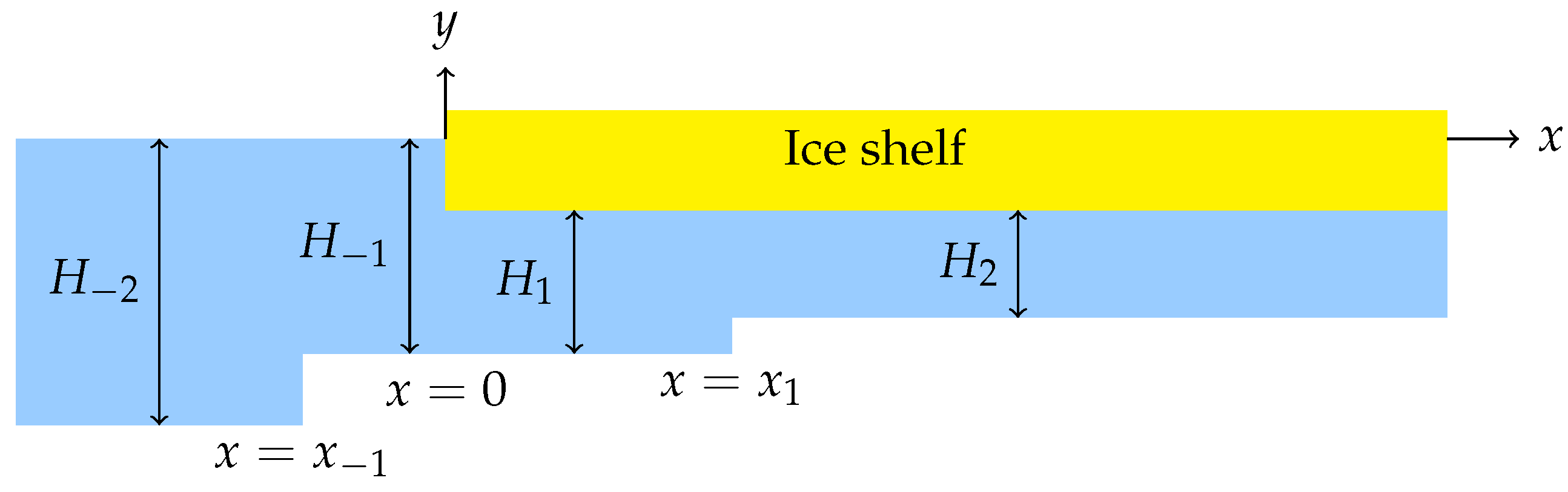
We considered here the case where there are three changes in depth. The first is outside the ice shelf, the second is at the ice shelf edge, and the third is under the ice shelf. We note that a change in depth under the ice shelf will occur due to the submergence of the ice shelf, even if the ocean depth remains constant. The ice shelf edge is assumed at
, and the changes in depths occur at
(in the open water) and
(under the ice shelf). This situation is shown in
Figure 2. The depths are
for
,
for
,
for
, and
for
. We are interested primarily in one change in depth, which we want to allow to be either before or under the ice shelf. The current situation covers both cases in one formulation and computer code.
When solving the differential equation for the system, we divided it into four different regions. Each region has different properties, such as thickness, Young’s modulus, etc. Since these properties are constant in each region, the equation written separately in each region is to be solved. Once each region has been solved, we are left with unknown coefficients, which can be determined by applying the boundary conditions. By applying the appropriate boundary conditions, we can solve for the coefficients and obtain a complete solution to the system.
The entire system can be described by the following equations for the four regions.
Note that we assumed that the ice shelf has a constant thickness and other properties. The current formulation could be extended straightforwardly to more complicated problems. The solution can be written as
The wavenumbers are given as follows. In the open water,
and
and
are three of the roots of the equations
and
The roots come in plus and minus pairs. We chose only one of each pair as follows. The pure imaginary root was chosen to have a positive imaginary part and was labelled or whereas the roots with a nonzero real part were chosen to have a negative real part and were labelled or . Note that these will be complex conjugates. Therefore, there are only three real variables to describe the three roots, as would be expected since the equations have only three real parameters.
The statement “we are imposing conditions at infinity” refers to the idea that, when we solve certain mathematical problems, we often need to consider what happens to the solution as we move further away from the origin or from some other point interest. In other words, we are interested in the behaviour of the solution "at infinity." In our specific problem, we are solving a wave-type equation, and we want to impose certain conditions on the solution to uniquely determine it.
The first condition is that “the solution cannot grow”. This condition means that the solution must not become arbitrarily large as we move further away from the origin. This eliminates two possible solutions to the equation because they would grow without bounds as we move away from the origin. The second condition is that “the wave is outgoing”. This condition means that the wave travels away from the origin rather than towards it. This condition is related to the Sommerfeld radiation condition, a set of conditions often used in solving wave equations to ensure that the solution represents a physically realistic wave. The Sommerfeld radiation condition, named after the German physicist Arnold Sommerfeld, is a mathematical criterion that describes how waves propagate in unbounded media, such as infinite space. Specifically, it sets a requirement on the field’s behaviour at infinity for it to represent a radiating source. In this case, the outgoing condition allows us to uniquely choose one of the solutions associated with the imaginary root of the equation.
We can see that we have twelve unknowns, and we, therefore, require twelve equations. We obtain these as follows. We require that, at each boundary, the potential is equal, i.e.,
,
, and
. This condition leads to the following three equations:
We also have continuity of flux so that
,
, and
. This condition leads to the following three equations:
The remaining six equations come from the plate conditions. In particular, the bending moment and shear force must vanish at the ice shelf edge and be continuous at
. Moreover, the displacement and first derivative must also be continuous at
. Therefore,
The equation for the displacement is
The six remaining equations are therefore (following from Equation (15))
The system of equations is linear, reflecting our assumption of linear differential equations. There are twelve linear equations in the twelve unknowns, which are solved straightforwardly. The solution can be thought of as a kind of finite element in which the elements are simply the underlying solutions, which generalise the beam finite elements. The solution is exact, up to the assumptions of the model.
4. Time-Domain Solutions
Time and frequency-domain simulations are essential tools in engineering and scientific analysis. However, time-domain simulation provides more information than frequency-domain simulation for several reasons. Time-domain simulation provides information about the behaviour of a system over time. It allows us to observe how a system responds to a given input signal or evolves over time under certain conditions. This information is critical in understanding the transient response of a system, which a frequency-domain simulation cannot fully capture. Frequency-domain simulation, on the other hand, provides information about the behaviour of a system at different frequencies. It allows us to observe how a system responds to sinusoidal inputs of different frequencies and how it attenuates or amplifies those frequencies. However, it cannot provide information about the system’s transient behaviour, which is vital in many applications. Moreover, the time-domain simulation can capture a wide range of behaviours that the frequency-domain simulation cannot. For example, time-domain simulation can simulate complex systems with varying inputs, whereas frequency-domain simulation is limited to linear systems with sinusoidal inputs. The time-domain simulation can also capture time-varying characteristics, such as frequency modulation or amplitude modulation, which cannot be accurately represented in the frequency domain.
We are particularly interested in simulating the motion in the time domain. The formula is given by
Note that is the wave number in the left-hand incident region. The integral is with respect to k so that, at , if the reflection were zero, the integral would be a straightforward Fourier transform of f.
In what follows, we will consider
f to be of the form
for which we know the Fourier transform explicitly. While the solution that we calculate is much more complicated than a simple Fourier transform, we have an analytic expression for the solution that we can use to validate our results in the zero reflection limit. Our choice of a Gaussian function (a bell-shaped curve that describes the distribution of many natural phenomena) has several advantages for Fourier transforms. A Gaussian function is infinitely differentiable, meaning it has no abrupt changes or discontinuities in its derivatives. This property is beneficial for Fourier transforms because it reduces the presence of high-frequency artefacts in the transformed signal, resulting in a smoother spectrum. The Fourier transform of a Gaussian function is also a Gaussian function, meaning it is highly localised in both time and frequency domains. This property allows for precise localisation of signals in both domains and can be helpful in applications where signal localisation is critical. The Gaussian function has the minimum possible product of the standard deviations of its Fourier transform and itself, which satisfies the uncertainty principle in Fourier analysis. This principle states that the more localised a signal is in time, the more spread out it will be in frequency and vice versa. The Gaussian function strikes a balance between time and frequency localisation and can extract features of a signal without losing too much information.
5. Results
When presenting scattering results for the wave–ice shelf system, choosing an appropriate parameter to express the results is essential. In this case, we decided to show the results in terms of energy rather than displacement. This choice was made because energy is a more fundamental quantity conserved in the system. At the same time, displacement is a secondary quantity dependent on factors such as ice shelf thickness and ocean depth. By presenting the results in terms of energy, we can provide a more accurate and meaningful representation of the system’s behaviour. Additionally, energy is a more physically relevant parameter when considering the effects of wave–ice shelf interactions. It reflects the amount of energy transmitted, absorbed, or scattered by the ice shelf. For this reason, rather than plotting the reflection and transmission coefficients, which, for changes in depth and ice shelves, can be misleading, we instead plot the transmitted and reflected energies (normalised by incident energy), which are given by
Note that they represent the normalised amount of energy reflected and transmitted and must sum to unity.
We considered four different depth changes: the first is constant depth, the second is a depth change before the ice shelf, the third is a depth change at the ice shelf, and the last case is a depth change both before and after. The reflected and transmitted energies are shown in
Figure 3. This figure illustrates the behaviour of energy transmission in the ice shelf water cavity system as a function of wave frequency. The graphs show that the energy is almost entirely transmitted and coupled with vibrational waves in the cavity for long-period waves. However, as the frequency of the waves increases, the ice shelf begins to reflect energy, with a clear transition occurring at a frequency of approximately 0.02 (corresponding to a period of 50 s). This trend continues as the frequency increases, but even at a frequency of 0.1, a significant amount of energy remains in the ice shelf. Overall, these figures demonstrate the complex and frequency-dependent nature of energy transmission in the ice shelf water cavity system, highlighting the importance of understanding these dynamics for accurately predicting the behaviour of the ice shelf under changing environmental conditions.
It can be observed that there is a clear correlation between changes in depth and the amount of energy transmitted. Specifically, it can be seen that the depth changes lead to a reduction in the amount of energy transmitted. Additionally, the figures also demonstrate that the change in depth before or after the shelf causes resonances, which are waves that bounce between the changes in depths. Finally, the step located before the shelf appears to have the most significant blocking effect, which could have implications for shielding ice shelves from ocean waves.
One interesting characteristic of ocean waves is that they often move in wave packets. A wave packet is a group of waves that travel together and have a similar wavelength and frequency. This grouping of waves can occur naturally as a result of interactions between different waves or as a result of other environmental factors. It therefore makes sense to simulate the response to such wave packets.
Figure 4,
Figure 5,
Figure 6 and
Figure 7 give the corresponding time-dependent motion of the ice shelf for an incident wave pulse, given by Equation (
20), with
(which corresponds to a peak period of
s), frequency
s
(for a water depth of 300 m), and
. The red dashed line is for illustration only and gives an idea of the depth in each case. These animations show the strong coupling between the open water waves and the ice shelf.
Figure 8 shows the time history of the ice shelf displacement for
Figure 4,
Figure 5,
Figure 6 and
Figure 7 at the ice shelf edge and 2000 m from the ice shelf edge.
The time-domain solutions of a wave propagation phenomenon are often best visualised through animations provided as
Supplementary Material. In this particular scenario, an energy packet strikes an ice shelf, causing it to vibrate significantly. As the energy packet travels through the ice shelf, some waves are reflected, while some are transmitted through the medium. The reflection and transmission of the wave alter its wavelength and shape, further influencing the ice shelf’s vibrations. Moreover, the group velocity of the wave in the ice shelf is much greater than that in the surrounding fluid, which adds to the phenomenon’s complexity. These observations highlight the importance of visual aids in understanding and interpreting wave propagation and its effects on the medium that it travels through.


