Abstract
This study investigates the ability of a new hybrid neuro-fuzzy model by combining the neuro-fuzzy (ANFIS) approach with the marine predators’ algorithm (MPA) in predicting short-term (from 1 h ahead to 1 day ahead) significant wave heights. Data from two stations, Cairns and Palm Beach buoy, were used in assessing the considered methods. The ANFIS-MPA was compared with two other hybrid methods, ANFIS with genetic algorithm (ANFIS-GA) and ANFIS with particle swarm optimization (ANFIS-PSO), in predicting significant wave height for multiple lead times ranging from 1 h to 1 day. The multivariate adaptive regression spline was investigated in deciding the best input for prediction models. The ANFIS-MPA model generally offered better accuracy than the other hybrid models in predicting significant wave height in both stations. It improved the accuracy of ANFIS-PSO and ANFIS-GA by 8.3% and 11.2% in root mean square errors in predicting a 1 h lead time in the test period.
1. Introduction
Significant wind wave height (SWH) is important for predicting seaquakes, tsunamis, and tropical cyclones; wave period and wave length is also needed for ships, maritime structures, and other business [1]. Accurate short-term SWH measurements are essential for planning protective measures against tsunamis, hydraulic structures, and wave energy facilities [2,3]. Hourly estimation of SWH is essential for short-term management, such as power generation [4]. Prediction of ship movements, construction of maritime structures, dredging operations, and disaster warnings are all examples of marine engineering that benefit from accurate real-time predictions of SWH characteristics. However, due to natural waves’ unpredictable and irregular nature, predicting wave power and building wave power plants is difficult [2]. The height of the waves is affected by environmental factors and climatic variations [5]. Wind causes waves and is the most important meteorological factor in determining wave height. The accuracy of weather forecasts is affected by the non-stationarity and non-linearity of wind and wave properties [6]. In early wave models, nonlinear interactions and energy dissipation were not adequately accounted for, resulting in unpredictable wind fields that made predictions difficult [4]. Many wave height prediction methods rely on semi-analytical approaches such as the Pierson–Neumann–James and Sverdrup–Munk–Bretschneider methods. However, these cannot provide sufficient information about the surface waves [3]. Numerical models are widely used for wave prediction. However, due to the large amount of data and the complexity of the calculations, they require high-performance computers and a considerable amount of time [7,8]. Although numerical models are useful for simulating the interaction between flow and structure, they may not be practical in critical situations where fast solutions are required [9].
Rahimian et al., 2022 [10] performed atmospheric simulations using weather and research forecasts (WRF) and compared the results with meteorological observations. Their results show that using the Mellor–Yamada–Nakanishi–Niino (MYNN) scheme for the planetary boundary and surface layers had the best performance for stations over water, while using the Mellor–Yamada–Janjic scheme for the planetary boundary and Eta-like surface layers had the best performance for stations over land. Lira-Loarca et al. [11] studied the wave hazard in the Mediterranean Sea using long-term hourly data and an unstructured grid wave model. Their results show that an SPI of 3 and 5 at the beginning and at the peak of the storm, respectively, leads to an SPI of 3–5, depending on the characteristics and socioeconomic importance of the coastal sections. Myslenkov et al. [12] studied the wind wave height in the Black Sea using different models. They concluded that for an SWH range of 0 to 3 m, the error does not exceed 0.5 m. However, for a SWH range of 3–4 m, the error increased significantly to −2 or −3 m. The quality of wave prediction was evaluated for several storm cases. Raj et al. [13] performed wind wave simulations in the Indian Ocean. Their results show that all wave simulations have significant errors at low wind speeds compared to medium and strong winds, regardless of the error in the wind forecast.
Advances in AI have enabled the widespread use of soft computing techniques to predict SWH. These methods are more efficient and versatile than their linear counterparts because they can represent nonlinear waves without requiring knowledge of input–output connections. Soft computing models have developed rapidly and are widely used as computation time decreases. Several soft computing techniques such as the RBM-DBN hybrid model, the BMA-MARS/RF/GBRT ensemble approach, the DBN-IF model, the En- RLMD-RF ensemble method, LSTM and GRU networks, and the CLTS-Net deep neural network model have been studied and found to be good at predicting significant wave height. Several methods were used to predict the SWH. The Restricted Boltzmann Machine (RBM) and the conventional Deep Belief Network (DBN) model were used in a hybrid form by Zhang and Dai [14] to predict the SWH on an hourly basis. According to their results, the hybrid model could predict the short-term maximum wave height with a relative error of less than 26%. Adnan et al. [15] used a Bayesian Model Averaging (BMA) ensemble strategy that included multivariate adaptive regression splines (MARS), random forests (RF), and gradient-boosted regression trees (GBRT). Specifically, they discovered that the BMA model predicted SWH up to six days in advance with slightly higher accuracy than previous techniques. The short-term wave height prediction was the focus of Li and Liu’s model [16] DBN-IF, a mixture of the dynamic Bayesian network and information flow. Their results showed the superior performance of the proposed DBN-IF model in predicting SWH. Ali et al. [15] proposed an ensemble local mean decomposition combined with random forest (En- RLMD-RF) to predict the short-term SWH. The results showed that the En- RLMD-RF model outperformed its benchmarks in prediction accuracy. Long short-term memory (LSTM) networks and recurrent gating networks (GRU) were two of the recurrent neural networks (RNN) that Feng et al. [17] investigated to predict SWH. Their results showed that gating-based LSTM and GRU networks performed better than conventional RNNs. Recently, a deep neural network model called CLTS-Net was developed by Li et al. [18] to predict SWH. Their results show that the CLTS-Net can simultaneously capture the temporal relationships in the data, which enables accurate prediction of future large wave heights.
The generalization capability and gradient-based parameter learning of soft computing algorithms still have limitations despite their superior accuracy in predicting significant wave height [5,19,20]. Therefore, reliance on a single machine learning approach can increase statistical variance and uncertainty due to limited input data for wave parameter prediction. To address this problem, the results of several different models can be combined using a multi-model approach. In this study, the performance of a refined neuro-fuzzy method was evaluated in conjunction with the algorithm used by marine predators. Adaptive Neuro-Fuzzy Inference System (ANFIS), ANFIS with genetic algorithm (ANFIS-GA), and ANFIS with particle swarm optimization were compared with this novel hybrid machine learning approach (ANFIS-MPA) (ANFIS-PSO). Half-hour time series data and a prediction method that looks several steps into the future were used for the analysis. This study is innovative in using the ANFIS-MPA approach to make multi-step predictions for SWH. Section 2 discusses the use of soft computing models and details the study area and data collection. Section 3 provides the main results and examines their implications for extending the newly tested model to additional climatic conditions. Section 4 summarizes the main results of this paper.
2. Case Study
For this study, two buoy sites were selected for wave monitoring in Queensland, namely the Cairns buoy and the Palm Beach buoy (Figure 1). The Cairns buoy is located in southeast Queensland near Cairns with a 12 m monitoring depth at coordinates 16°43.830′ south latitude and 145°42.910′ east longitude. In contrast, the Palm Beach buoy is located in far north Queensland near Sydney with 23 m monitoring depth at coordinates 28°05.956′ south latitude and 153°29.073′ east longitude. The Queensland Government Meteorological Department collects significant wave height data at 30 min intervals. For this study, significant wave height data were downloaded from the Queensland Government website (https://www.data.qld.gov.au/dataset, accessed on 7 March 2023) at 30 min intervals for both buoy locations from 1 January 2022 to 31 December 2022. A brief statistical summary of the data used is provided in Table 1. This study uses the average hourly data with a split ratio of 75% training and 25% test to apply models to predict single-level and multi-level significant wave height (SWH). To predict SWH, only historical data of the SWH variable of both stations were used as inputs; it is worth noting that both stations were not connected as one was on the northern side, whereas the other station was on the southeast side of Queensland, as mentioned above. Data from 1 January 2022 to 30 September 2022 was adopted as the training dataset, whereas data from 1 October 2022 to 31 December 2022 was adopted as the testing dataset.
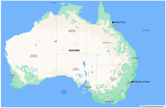
Figure 1.
Case study area for significant wave height modeling representing Station 1 (Cairns) and Station 2 (Palms Beach).

Table 1.
The statistical parameters of the applied data.
3. Methods
3.1. Multivariate Adaptive Regression Splines (MARS)
The Multivariate Adaptive Regression Splines model (MARS) allows for revealing a hidden nonlinear pattern in a dataset with many variables [21,22,23]. In this way, obtaining the estimator defined using a single method is possible, and combining several statistical methods is unnecessary. The basis of this method is based on functions called basis functions, which can be expressed for each explanatory variable as follows (Equation (1)):
where t is called a node, and in practice, one of its observations is an explanatory variable. These functions are spline functions found in the reciprocal pair node t.
The general shape of the MARS model is described by Equation (2):
In this equation, Y is the estimated value of the response variable (here, it is estimated significant wave height), X is the vector ck of the basis function, and Bk is the explanatory variables or the equal elements of the Parajets coefficient determined by minimizing the sum of the squares of the residuals. Each basis function can be a form of a linear spline function or the product of two or more of them, indicating mutual effects. In the model MARS, the space of explanatory variables is divided into several separate regions by certain knots, which gives the greatest reduction of the sum of squared errors [24,25,26].
MARS model fitting is performed in two stages. Many basis functions with different nodes are gradually added to the model in the advanced stage. This process results in a more complicated model that is more fitting. In the second stage, the regression removal stage, the basis functions that are less important and influential for the estimation are removed. Finally, the most accurate model is selected based on the minimum Generalized Cross Validation (GCV) criterion. GCVk is assumed as the value of GCV for k of the model in the elimination phase. This quantity is defined by Equation (3):
where is the estimated model in the step of the elimination step; C(k) is the number of model sentences in the step + λm, where m represents the number of spline function nodes in the model; and λ is called the smoothing parameter and is usually chosen between 2 and 4 in practice [27,28].
3.2. Adaptive Neuro-Fuzzy Inference System (ANFIS)
Networks based on an adaptive neuro-fuzzy inference system [29,30,31] provide a practical approach to approximate functions. Fuzzy set theory is tailored to automated systems that efficiently manage complex operations [32,33]. Individual membership values should be used to map the elements of a fuzzy set to function theory. The components of the fuzzy theory can have real values anywhere in the range [0, 1]. Fuzzy inference systems (FIS) and ANFIS models rely heavily on partitioning the available data into training and test sets. The general structure of ANFIS is shown in Figure 2. In this present study, previous significant wave heights (SWH) were used as inputs, while the output f is the SWH value at t + 1 (one hour ahead) to t + 24 (one day ahead). In Figure 2, the p, q, and r refer to the consequent parameters, while the parameters of the membership functions (e.g., A and B, as seen from the figure) are called premise parameters. All these parameters were optimized using GA, PSO, and MPA algorithms, which are briefly explained in the following sections. In Figure 2, W refers to the membership degree corresponding to each value set of x and y inputs. In this study, x and y can be assumed as SWHt and SWHt−1.
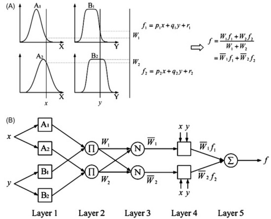
Figure 2.
Description of the ANFIS method: (A) fuzzy inference and (B) corresponding ANFIS structure.
3.3. Optimization Algorithms
3.3.1. Genetic Algorithm (GA)
Genetic algorithms (GAs) are machine learning and optimization methods like neural networks. In genetic programming, the existing blocks are first defined, which include the input and target variables and their connection function. Then, the appropriate structure of the model and its coefficients are determined [34,35,36]. This method includes a correlation equation between the input and output variables. Therefore, it can automatically select the appropriate variables of the model and delete unrelated variables that cause input dimension reduction [37,38,39]. The selection of appropriate model inputs is one of the most important issues that should be considered in this method. This issue is even more important when secondary input data are also used. This is because the presentation of unrelated input data leads to a decrease in the model’s accuracy and to the creation of more complicated models, the interpretation of which is associated with more difficulties. In engineering applications, genetic programming is often used for modeling problems related to determining the structure of phenomena. The step-by-step process of genetic programming is as follows:
- 1.
- An initial set of composite functions indicating predictive models is considered randomly.
- 2.
- Each person in the above population is evaluated with appropriate functions.
- 3.
- For each production, the following steps are followed to select a new population:
- (a)
- One of the transitions, mutation, and copy operators is selected.
- (b)
- An appropriate number of individuals from the current community are selected.
- (c)
- The selection operator is used to generate the descendants.
- (d)
- The named descendant enters a new society.
- (e)
- The considered model is evaluated using various adjustments.
- 4.
- The third step is repeated until the maximum production is reached.
In this method, no dependent relation is considered at the beginning of the process. Therefore, it can optimize the structure of the model and its components [40,41].
3.3.2. Particle Swarm Optimization (PSO)
The PSO algorithm was developed by Kennedy and Eberhart [42] and is based on the activity of swarms of bees searching for flowers to pollinate. A swarm consists of particles, and each particle represents an answer to an optimization problem. This method starts with a collection of solutions initially in random locations and moving at random speeds. Particle swarm optimization (PSO) uses particles moving in hyperspace to find optimal solutions. Over time, these solutions gain knowledge through their own experiences and those of their peers. Each atom remembers its highest fitness level in the cloud, which it calls its pbest. The gbest or global best is the best value ever achieved by a particle in the population. Each particle in the system rapidly moves to its pbest and gbest positions when the PSO algorithm is run. For this purpose, the new velocity of each particle is determined by its distance from the pbest and gbest positions. Then, a new velocity value for that particle is calculated by randomly weighing the two best velocities, pbest and gbest, to determine its next place in the following iteration [43,44,45].
The relative simplicity of the process with only two equations is one of the main advantages of PSO over many other optimization techniques (i.e., the equation of motion and the equation for updating the velocity). The actual motion of the particles is determined via their unique velocity vector, which is used in the first equation. Conversely, the second determines how the velocity vector must shift to account for the presence of opposing forces [46,47]. The convergence rate of the PSO algorithm is further improved by introducing the inertia weight (w) (Figure 3).
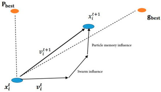
Figure 3.
Optimization procedure of particle swarm optimization.
3.3.3. Marine Predators Algorithm (MPA)
The MPA is a meta-heuristic (MH) algorithm based on the hunting techniques of marine predators. Like the other algorithms of MH, the MPA first explores the search space and obtains random intervals of initial solutions using a prey search technique. The primary structure of the algorithm is that the current position determines the future position of the solution [48,49]. Marine predators use Lévy and Brownian search techniques when searching for food, switching between the two depending on the availability of potential meals. In locations with lower prey concentration, predators use the Lévy movement. Instead, Brownian motion is used [50,51] when numerous potential victims are available. This study randomly chose initial solutions, updating the positions using Equation (4) as follows:
where ymax and ymin are the upper and lower bounds of the design variables, respectively, and rand is also a random vector in the range [1 0]. In the MPA, there are two main matrices, the best-fit predator matrix (Best/Elite) and the prey matrix (Prey), given in Equations (5) and (6).
where y is a vector of the most appropriate hunters repeated n-times to organize the elite matrix. n and d refer to the number and dimensions of search factors. Elite is updated after each iteration of the prey by replacing the better hunters. The matrix is the basis on which the hunters update their position, and its dimensions are the same as those of the elite matrix. The prey matrix is expressed as follows:
In y-ij., j-th. is next for i-th. by prey. MPA: During the search, it repeatedly uses random variables and operators to prevent the algorithm from getting stuck in local minimal points [52]. To better understand the MPA method, the structure of the proposed algorithm is shown in the flowchart in Figure 4.
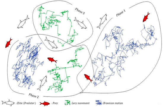
Figure 4.
MPA optimization flowchart.
3.4. Development of Hybrid ANFIS Methods
To improve the accuracy of ANFIS method in predicting SWH for multiple horizons, three metaheuristic algorithms, PSO, GA, and MPA, were used to optimize the consequent (p, q, and r) and premise parameters (membership functions). In this present study, inputs are SWHt, SWHt−1, and SWHt−2, referring to the SWH at time t, t − 1, and t − 2, where t is hour and output is SWH at time t + 1 (one hour ahead) to t + 24 (one day ahead). Each input has Gaussian membership functions, and each membership function has two parameters: mean and standard deviation. Three metaheuristic algorithms, i.e., PSO, GA, and MPA, were used for optimizing linear (consequent) and nonlinear (premise) parameters of ANFIS. The procedure for developing hybrid ANFIS models, including ANFIS-PSO, ANFIS-GA, and ANFIS-MPA, is depicted in Figure 5.
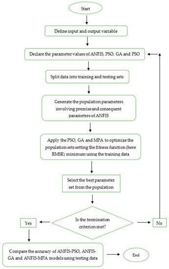
Figure 5.
The development of hybrid ANFIS models.
3.5. Accuracy Assessment
To achieve better prediction of SWH using historical SWH values as input, the primary goal of this work was to use a novel hybrid neuro-fuzzy approach: ANFIS-MPA. The root means square error, mean absolute error, and coefficient of determination (R2) were compared with two other hybrid ANFIS techniques, ANFIS-GA and ANFIS-PSO, to evaluate the results. Data from two sites were used for the applications to ensure that the techniques worked as intended. There are many ways to display the RMSE, MAE, and R2 statistics, which are demonstrated as follows [53,54,55,56]:
where are calculated, observed, mean significant wave height, and the number of data, respectively.
4. Development of Hybrid ANFIS-PSO, ANFIS-GA, and ANFIS-MPA Models
In the final model developed, MARS was used to determine the best input combination, i.e., the best scenario for predicting SWH is evaluated. Each scenario considers different lagged SWH values. Then, all input combinations are analyzed for three hybrid ANFIS models, including ANFIS-PSO, ANFIS-GA, and ANFIS-MPA. Three statistical indices, including RMSE, MAE, and R2, are used for comparison suggestions.
5. Results and Discussion
This section compares the results of the MPA-based neuro-fuzzy approach in predicting significant wave heights for multiple horizons from t + 1 (one hour ahead) to t + 24 (one day ahead) with other hybrid neuro-fuzzy methods.
5.1. Results
In this study, we first apply the MARS method to determine the best input combination. The goal was to investigate whether this method can be applied to determine the best scenario for predicting SWH. This was then evaluated via hybrid ANFIS methods for all input combinations. The training and test results of the method MARS are shown in Table 2 for the first station. As seen from the input combinations, three lagged inputs were used because inputs beyond this lag did not improve the prediction accuracy, and our goal was to predict SWH for multiple horizons from t + 1 to t + 24. Table 3 shows that adding earlier lags slightly improves the accuracy of MARS. Therefore, three delayed inputs were selected as the best input combination. Then, this combination was used to predict SWH for other periods. As expected, the model’s accuracy deteriorates as the prediction horizon increases. The RMSE and MAE decreased from 0.0325 and 0.0232 to 0.1410 and 0.1076, and R2 increased from 0.9748 to 0.5201 over the test period.

Table 2.
Training and test statistics of the models for multiple steps ahead SWH predictions—MARS for Station 1.

Table 3.
Training and test statistics of the models for multiple steps ahead SWH predictions—ANFIS-PSO for Station 1.
Table 3, Table 4 and Table 5 summarize the training and testing results of the hybrid models ANFIS-PSO, ANFIS-GA, and ANFIS-MPA in predicting the SWH of the first station. The accuracy of the implemented methods is consistent, and all three methods provide the best performance for the third input combination. The model ANFIS-MPA showed the lowest RMSE (0.0277) and MAE (0.0192) and the highest R2 (0.9831) during the test period; followed by ANFIS-GA with an RMSE, MAE, and R2 of 0.0302, 0.0216, and 0.9787; and ANFIS-PSO with an RMSE, MAE, and R2 of 0.0312, 0.0226, and 0.9753. From t + 1 (1 h ahead) to t + 24 (1 day ahead), the accuracy of ANFIS-MPA decreases significantly; the RMSE, MAE, and R2 range from 0.0277, 0.0192, and 0.9831 to 0.1344, 0.1019, and 0.5833, respectively. At all forecast horizons, ANFIS-MPA is superior to the other hybrid methods. The improvement in RMSE of ANFIS-GA and ANFIS-PSO at the 1 h lead time test period is 11.2% and 8.3%, respectively. In contrast, the corresponding improvement at one day lead time (t + 24) is 3.38% and 0.59%.

Table 4.
Training and test statistics of the models for multiple steps ahead SWH predictions—ANFIS-GA for Station 1.

Table 5.
Training and test statistics of the models for multiple steps ahead SWH predictions—ANFIS-MPA for Station 1.
Table 6 shows the training and test results of the method MARS for the first station. Again, accuracy for this station decreased slightly when delayed inputs were added. Accuracy decreased significantly when the prediction horizon was increased from 1 h to 1 day (t + 24). The RMSE, MAE, and R2 range from 0.1067, 0.0824, and 0.9635 to 0.2928, 0.2029, and 0.7303 in the test period. The best accuracy is obtained by the model with inputs Hst, Hst-1, and Hst-2 with the lowest RMSE (0.1067) and MAE (0.0824) and the highest R2 (0.9635) in the test period.

Table 6.
Training and test statistics of the models for multiple steps ahead SWH predictions—MARS for Station 2.
The training and test results of the hybrid ANFIS methods in predicting SWH at the second station are shown in Table 7, Table 8 and Table 9. This station also shows consistent accuracy of the implemented methods with MARS. The best performance is obtained at the third input combination. Again, ANFIS-MPA outperforms ANFIS-PSO and ANFIS-GA in the 1 h SWH prediction with the lowest RMSE (0.0689) and MAE (0.0475) and the highest R2 (0.9847) in the test period. The use of ANFIS-MPA improves the RMSE accuracy of ANFIS-PSO by about 7% in predicting SWH 1 h ahead. Similar to the first station, the accuracy of the hybrid methods decreases significantly. For example, the RMSE, MAE, and R2 of ANFIS-MPA range from 0.0689, 0.0475, and 0.9847 to 0.2640, 0.1962, and 0.7735, respectively, for forecast horizons t + 1 to t + 24. The ANFIS-MPA outperforms the other hybrid methods at all forecast horizons.

Table 7.
Training and test statistics of the models for multiple steps ahead SWH predictions—ANFIS-PSO for Station 2.

Table 8.
Training and test statistics of the models for multiple steps ahead SWH predictions—ANFIS-GA for Station 2.

Table 9.
Training and test statistics of the models for multiple steps ahead SWH predictions—ANFIS-MPA for Station 2.
The hybrid neuro-fuzzy and MARS models for predicting SWH are compared in Figure 6 and Figure 7 using scatter plots. The MPS-based ANFIS has the least scattered predictions, with the fitting equation closer to the exact line (y = x) and the highest R2 in both stations. The models with three inputs (best models) are compared using Taylor diagrams in Figure 8 and Figure 9. This type of graph is very useful for observing the accuracy of the models based on RMSE, standard deviation, and correlation. The plots show that the MPA-based ANFIS has the highest correlation and the lowest squared error in predicting the SWH of both stations. The violin charts in Figure 10 and Figure 11 compare the SWH predictions and observations distributions. The figures show that the mean, median, and distribution of the MPA-based ANFIS are more like the observed values. Figure 12 illustrates the average RMSE and MAE errors of all implemented models in predicting the SWH of both stations. It is clearly seen from the bar charts that the ANFIS-MPA has fewer RMSE and MAE errors in the short-term prediction of SWH in both sites.
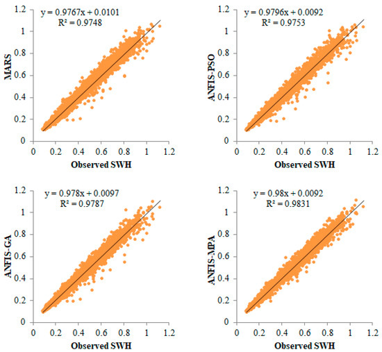
Figure 6.
Scatterplots of the observed and predicted SWH by different models in the test period using the best input combination at Station 1.
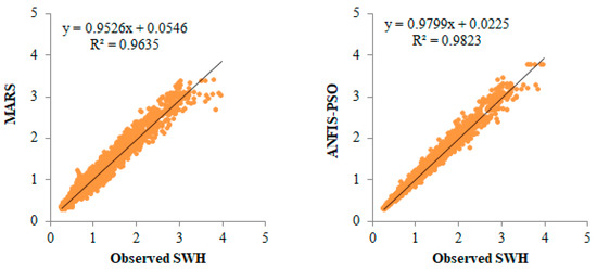
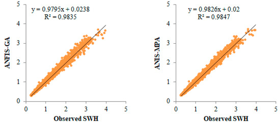
Figure 7.
Scatterplots of the observed and predicted SWH by different models in the test period using the best input combination at Station 2.
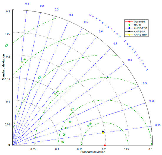
Figure 8.
Taylor diagrams of the predicted SWH by different models using the best input combination at Station 1.
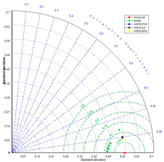
Figure 9.
Taylor diagrams of the predicted SWH by different models using the best input combination at Station 2.
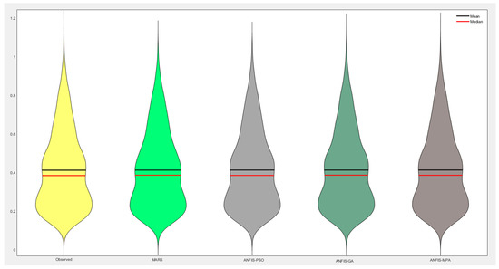
Figure 10.
Violin charts of the predicted SWH by different models using the best input combination at Station 1.
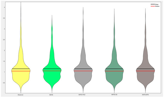
Figure 11.
Violin charts of the predicted SWH by different models using the best input combination at Station 2.
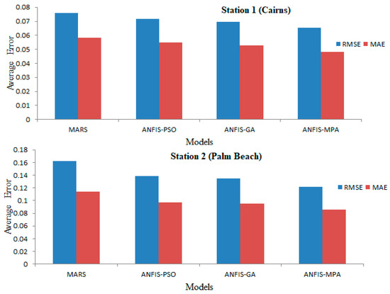
Figure 12.
Average RMSE and MAE of the applied models in predicting SWH using all models for all input combinations during test period of both stations.
5.2. Discussion
This study uses a new hybrid neuro-fuzzy method (ANFIS-MPA) to predict SWH using previous values as input. The results are compared with other hybrid neuro-fuzzy models. The MPA-based model is observed to outperform the other models in predicting SWH for multiple horizons from 1 h to 1 day.
The best input combination is investigated using the MARS method. Next, hybrid ANFIS methods are applied to the same scenarios to see if MARS is suitable for determining the best input combination in predicting SWH. A similar trend is observed between the MARS and hybrid ANFIS methods, indicating that the MARS can successfully determine the best input combination in SWH prediction. The comparison of the two stations shows that the methods are more successful in predicting SWH at the second station. The main reason could be the higher autocorrelation of SWG at the second station. These results are consistent with the previous literature [48,50].
It is observed that with the increasing horizon from 1 h to 24 h, the models’ accuracy highly deteriorates. However, the ANFIS-MPA generally provides superiority in such cases, which can be useful in monitoring SWH.
Machine learning allows us to find connections between physical parameters that we do not see or do not know. The formation of waves has a nonlinear and complex physical mechanism, and SWH is affected by different parameters, including wind speed, sea surface temperature, water depth, air humidity, and some other weather parameters. In this present study, only SWH data were used as inputs because of the unavailability of other influencing parameters.
6. Conclusions
This study examined the performance of a new hybrid neuro-fuzzy model, ANFIS-MPA, in predicting significant wave height in multiple horizons from 1 h to 1 day. Hourly data were obtained from two stations, Cairns and Palm Beach buoys, Australia. MARS as a simple tool was used to determine the best input of significant wave height for the much more complex hybrid ANFIS methods. This was also justified by employing hybrid methods for the same input combinations. It was observed that the MARS can be successfully used for selecting the best input combination in predicting significant wave height. The results of ANFIS-MPA were compared with those of the hybrid models ANFIS-PSO and ANFIS-GA. The results showed that the ANFIS-MPA model performed better than the other hybrid models in predicting significant wave height at both stations. At the second station, ANFIS-GA and ANFIS-PSO provided better accuracy than ANFIS-MPA for predicting the significant wave height 1 h ahead, while the latter model outperformed the ANFIS-GA and ANFIS-PSO for other forecasting horizons involving wave heights 2, 4, 8, 12, and 24 h ahead. Assessment criteria involving average RMSE and MAE and graphical inspections such as Taylor and Violin charts revealed that the ANFIS-MPA is superior to the other models in predicting SWH for multiple horizons. Overall results recommend the use of ANFIS-MPA in monitoring significant wave height for multiple time horizons, using only earlier values as inputs.
In this study, we used hourly data from two sites. The results can be generalized if data from other sites and other data intervals (daily or monthly) are used. The developed methods can also be compared with other hybrid machine learning methods to evaluate the accuracy of the implemented methods in predicting significant wave height. In this study, only previous SVH data were used as inputs, and in future studies, more effective parameters such as wind speed, sea surface temperature, water depth, and air humidity can be involved to develop more robust and accurate models in predicting SWH for multiple horizons.
Author Contributions
Conceptualization: R.M.A.I. and O.K.; formal analysis: R.M.A.I.; validation: O.K., X.C., T.S., A.K., S.S. and R.M.A.I.; supervision: O.K. and X.C.; writing—original draft: O.K., T.S., A.K., S.S. and R.M.A.I.; visualization: R.M.A.I. and T.S.; investigation: O.K., A.K. and T.S. All authors have read and agreed to the published version of the manuscript.
Funding
This research received no external funding.
Institutional Review Board Statement
Not applicable.
Informed Consent Statement
Not applicable.
Data Availability Statement
The data presented in this study will be available upon an interested request from the corresponding author.
Conflicts of Interest
There are no conflict of interest in this study.
References
- Gómez-Orellana, A.M.; Guijo-Rubio, D.; Gutiérrez, P.A.; Hervás-Martínez, C. Simultaneous short-term significant wave height and energy flux prediction using zonal multi-task evolutionary artificial neural networks. Renew. Energy 2022, 184, 975–989. [Google Scholar] [CrossRef]
- Huang, W.; Dong, S. Improved short-term prediction of significant wave height by decomposing deterministic and stochastic components. Renew. Energy 2021, 177, 743–758. [Google Scholar] [CrossRef]
- Fan, S.; Xiao, N.; Dong, S. A novel model to predict significant wave height based on long short-term memory network. Ocean Eng. 2020, 205, 107298. [Google Scholar] [CrossRef]
- Duan, W.Y.; Han, Y.; Huang, L.M.; Zhao, B.B.; Wang, M.H. A hybrid EMD-SVR model for the short-term prediction of significant wave height. Ocean Eng. 2016, 124, 54–73. [Google Scholar] [CrossRef]
- Kaloop, M.R.; Kumar, D.; Zarzoura, F.; Roy, B.; Hu, J.W. A wavelet—Particle swarm optimization—Extreme learning machine hybrid modeling for significant wave height prediction. Ocean Eng. 2020, 213, 107777. [Google Scholar] [CrossRef]
- Zhao, L.; Li, Z.; Qu, L.; Zhang, J.; Teng, B. A hybrid VMD-LSTM/GRU model to predict non-stationary and irregular waves on the east coast of China. Ocean Eng. 2023, 276, 114136. [Google Scholar] [CrossRef]
- Gicquel, L.Y.M.; Gourdain, N.; Boussuge, J.-F.; Deniau, H.; Staffelbach, G.; Wolf, P.; Poinsot, T. High performance parallel computing of flows in complex geometries. Comptes Rendus Mécanique 2011, 339, 104–124. [Google Scholar] [CrossRef]
- Bauer, P.; Dueben, P.D.; Hoefler, T.; Quintino, T.; Schulthess, T.C.; Wedi, N.P. The digital revolution of Earth-system science. Nat. Comput. Sci. 2021, 1, 104–113. [Google Scholar] [CrossRef]
- Di Sabatino, S.; Buccolieri, R.; Salizzoni, P. Recent advancements in numerical modelling of flow and dispersion in urban areas: A short review. Int. J. Environ. Pollut. 2013, 52, 172–191. [Google Scholar] [CrossRef]
- Rahimian, M.; Beyramzadeh, M.; Siadatmousavi, S.M. The Skill Assessment of Weather and Research Forecasting and WAVEWATCH-III Models During Recent Meteotsunami Event in the Persian Gulf. Front. Mar. Sci. 2022, 9, 834151. [Google Scholar] [CrossRef]
- Lira-Loarca, A.; Cáceres-Euse, A.; De-Leo, F.; Besio, G. Wave modeling with unstructured mesh for hindcast, forecast and wave hazard applications in the Mediterranean Sea. Appl. Ocean Res. 2022, 122, 103118. [Google Scholar] [CrossRef]
- Myslenkov, S.; Zelenko, A.; Resnyanskii, Y.; Arkhipkin, V.; Silvestrova, K. Quality of the Wind Wave Forecast in the Black Sea Including Storm Wave Analysis. Sustainability 2021, 13, 13099. [Google Scholar] [CrossRef]
- Raj, A.; Kumar, B.P.; Remya, P.G.; Sreejith, M.; Nair, T.M.B. Assessment of the forecasting potential of WAVEWATCH III model under different Indian Ocean wave conditions. J. Earth Syst. Sci. 2023, 132, 32. [Google Scholar] [CrossRef]
- Zhang, X.; Dai, H. Significant Wave Height Prediction with the CRBM-DBN Model. J. Atmos. Ocean. Technol. 2019, 36, 333–351. [Google Scholar] [CrossRef]
- Adnan, R.M.; Sadeghifar, T.; Alizamir, M.; Azad, M.T.; Makarynskyy, O.; Kisi, O.; Barati, R.; Ahmed, K.O. Short-term probabilistic prediction of significant wave height using bayesian model averaging: Case study of chabahar port, Iran. Ocean Eng. 2023, 272, 113887. [Google Scholar] [CrossRef]
- Li, M.; Liu, K. Probabilistic Prediction of Significant Wave Height Using Dynamic Bayesian Network and Information Flow. Water 2020, 12, 2075. [Google Scholar] [CrossRef]
- Feng, Z.; Hu, P.; Li, S.; Mo, D. Prediction of Significant Wave Height in Offshore China Based on the Machine Learning Method. J. Mar. Sci. Eng. 2022, 10, 836. [Google Scholar] [CrossRef]
- Ali, M.; Prasad, R.; Xiang, Y.; Jamei, M.; Yaseen, Z.M. Ensemble robust local mean decomposition integrated with random forest for short-term significant wave height forecasting. Renew. Energy 2023, 205, 731–746. [Google Scholar] [CrossRef]
- Li, S.; Hao, P.; Yu, C.; Wu, G. CLTS-Net: A More Accurate and Universal Method for the Long-Term Prediction of Significant Wave Height. J. Mar. Sci. Eng. 2021, 9, 1464. [Google Scholar] [CrossRef]
- Fernández, J.C.; Salcedo-Sanz, S.; Gutiérrez, P.A.; Alexandre, E.; Hervás-Martínez, C. Significant wave height and energy flux range forecast with machine learning classifiers. Eng. Appl. Artif. Intell. 2015, 43, 44–53. [Google Scholar] [CrossRef]
- Friedman, J.H.; Roosen, C.B. An introduction to multivariate adaptive regression splines. Stat. Methods Med. Res. 1995, 4, 197–217. [Google Scholar] [CrossRef]
- Zhang, W.; Goh, A.T. Multivariate adaptive regression splines and neural network models for prediction of pile drivability. Geosci. Front. 2016, 7, 45–52. [Google Scholar] [CrossRef]
- Dodangeh, E.; Choubin, B.; Eigdir, A.N.; Nabipour, N.; Panahi, M.; Shamshirband, S.; Mosavi, A. Integrated machine learning methods with resampling algorithms for flood susceptibility prediction. Sci. Total. Environ. 2020, 705, 135983. [Google Scholar] [CrossRef] [PubMed]
- Raja, M.N.A.; Shukla, S.K. Multivariate adaptive regression splines model for reinforced soil foundations. Geosynth. Int. 2021, 28, 368–390. [Google Scholar] [CrossRef]
- Kao, L.-J.; Chiu, C.C. Application of integrated recurrent neural network with multivariate adaptive regression splines on SPC-EPC process. J. Manuf. Syst. 2020, 57, 109–118. [Google Scholar] [CrossRef]
- Chen, W.-H.; Lo, H.-J.; Aniza, R.; Lin, B.-J.; Park, Y.-K.; Kwon, E.E.; Sheen, H.-K.; Grafilo, L.A.D.R. Forecast of glucose production from biomass wet torrefaction using statistical approach along with multivariate adaptive regression splines, neural network and decision tree. Appl. Energy 2022, 324, 119775. [Google Scholar] [CrossRef]
- Wang, L.; Wu, C.; Gu, X.; Liu, H.; Mei, G.; Zhang, W. Probabilistic stability analysis of earth dam slope under transient seepage using multivariate adaptive regression splines. Bull. Eng. Geol. Environ. 2020, 79, 2763–2775. [Google Scholar] [CrossRef]
- Sirimontree, S.; Jearsiripongkul, T.; Lai, V.Q.; Eskandarinejad, A.; Lawongkerd, J.; Seehavong, S.; Thongchom, C.; Nuaklong, P.; Keawsawasvong, S. Prediction of penetration resistance of a spherical penetrometer in clay using multivariate adaptive regression splines model. Sustainability 2022, 14, 3222. [Google Scholar] [CrossRef]
- Jang, J.-S.R.; Sun, C.-T.; Mizutani, E. Neuro-Fuzzy and Soft Computing: A Computational Approach to Learning and Machine Intelligence; Prentice-Hall: Upper Saddle River, NJ, USA, 1997. [Google Scholar]
- Karaboga, D.; Kaya, E. Adaptive network based fuzzy inference system (ANFIS) training approaches: A comprehensive survey. Artif. Intell. Rev. 2019, 52, 2263–2293. [Google Scholar] [CrossRef]
- Harandizadeh, H.; Jahed Armaghani, D.; Khari, M. A new development of ANFIS–GMDH optimized by PSO to predict pile bearing capacity based on experimental datasets. Eng. Comput. 2021, 37, 685–700. [Google Scholar] [CrossRef]
- Beiki, H. Developing convective mass transfer of nanofluids in fully developed flow regimes in a circular tube: Modeling using fuzzy inference system and ANFIS. Int. J. Heat Mass Transf. 2021, 173, 121285. [Google Scholar] [CrossRef]
- Ghenai, C.; Al-Mufti, O.A.A.; Al-Isawi, O.A.M.; Amirah, L.H.L.; Merabet, A. Short-term building electrical load forecasting using adaptive neuro-fuzzy inference system (ANFIS). J. Build. Eng. 2022, 52, 104323. [Google Scholar] [CrossRef]
- Holland, J.H. Genetic algorithms. Sci. Am. 1992, 267, 66–73. [Google Scholar] [CrossRef]
- Mirjalili, S. Genetic algorithm. In Evolutionary Algorithms and Neural Networks: Theory and Applications; Springer: Cham, Switzerland, 2019; pp. 43–55. [Google Scholar]
- Katoch, S.; Chauhan, S.S.; Kumar, V. A review on genetic algorithm: Past, present, and future. Multimed. Tools Appl. 2021, 80, 8091–8126. [Google Scholar] [CrossRef] [PubMed]
- Reddy, G.T.; Reddy, M.P.K.; Lakshmanna, K.; Rajput, D.S.; Kaluri, R.; Srivastava, G. Hybrid genetic algorithm and a fuzzy logic classifier for heart disease diagnosis. Evol. Intell. 2020, 13, 185–196. [Google Scholar] [CrossRef]
- Ilbeigi, M.; Ghomeishi, M.; Dehghanbanadaki, A. Prediction and optimization of energy consumption in an office building using artificial neural network and a genetic algorithm. Sustain. Cities Soc. 2020, 61, 102325. [Google Scholar] [CrossRef]
- Chen, R.; Yang, B.; Li, S.; Wang, S. A self-learning genetic algorithm based on reinforcement learning for flexible job-shop scheduling problem. Comput. Ind. Eng. 2020, 149, 106778. [Google Scholar] [CrossRef]
- Garud, K.S.; Jayaraj, S.; Lee, M.-Y. A review on modeling of solar photovoltaic systems using artificial neural networks, fuzzy logic, genetic algorithm and hybrid models. Int. J. Energy Res. 2021, 45, 6–35. [Google Scholar] [CrossRef]
- Sang, B. Application of genetic algorithm and BP neural network in supply chain finance under information sharing. J. Comput. Appl. Math. 2021, 384, 113170. [Google Scholar] [CrossRef]
- Eberhart, R.; Kennedy, J. Particle swarm optimization. In Proceedings of the IEEE International Conference on Neural Networks, Perth, WA, Australia, 27 November–1 December 1995; Volume 4, pp. 1942–1948. [Google Scholar]
- Poli, R.; Kennedy, J.; Blackwell, T. Particle swarm optimization: An overview. Swarm Intell. 2007, 1, 33–57. [Google Scholar] [CrossRef]
- Jain, M.; Saihjpal, V.; Singh, N.; Singh, S.B. An Overview of Variants and Advancements of PSO Algorithm. Appl. Sci. 2022, 12, 8392. [Google Scholar] [CrossRef]
- Pareek, C.M.; Tewari, V.K.; Machavaram, R.; Nare, B. Optimizing the seed-cell filling performance of an inclined plate seed metering device using integrated ANN-PSO approach. Artif. Intell. Agric. 2021, 5, 1–12. [Google Scholar] [CrossRef]
- Pradhan, A.; Bisoy, S.K.; Das, A. A survey on PSO based meta-heuristic scheduling mechanism in cloud computing environment. J. King Saud Univ.-Comput. Inf. Sci. 2022, 34, 4888–4901. [Google Scholar] [CrossRef]
- Kaur, M.; Dutta, M.K. Restoration and quality improvement of distorted tribal artworks using Particle Swarm Optimization (PSO) technique along with nonlinear filtering. Optik 2021, 245, 167709. [Google Scholar] [CrossRef]
- Faramarzi, A.; Heidarinejad, M.; Mirjalili, S.; Gandomi, A.H. Marine Predators Algorithm: A nature-inspired metaheuristic. Expert Syst. Appl. 2020, 152, 113377. [Google Scholar] [CrossRef]
- Soliman, M.A.; Hasanien, H.M.; Alkuhayli, A. Marine predators algorithm for parameters identification of triple-diode photovoltaic models. IEEE Access 2020, 8, 155832–155842. [Google Scholar] [CrossRef]
- Ramezani, M.; Bahmanyar, D.; Razmjooy, N. A new improved model of marine predator algorithm for optimization problems. Arab. J. Sci. Eng. 2021, 46, 8803–8826. [Google Scholar] [CrossRef]
- Ikram, R.M.A.; Ewees, A.A.; Parmar, K.S.; Yaseen, Z.M.; Shahid, S.; Kisi, O. The viability of extended marine predators algorithm-based artificial neural networks for streamflow prediction. Appl. Soft Comput. 2022, 131, 109739. [Google Scholar] [CrossRef]
- Houssein, E.H.; Hassaballah, M.; Ibrahim, I.E.; AbdElminaam, D.S.; Wazery, Y.M. An automatic arrhythmia classification model based on improved marine predators algorithm and convolutions neural networks. Expert Syst. Appl. 2022, 187, 115936. [Google Scholar] [CrossRef]
- Mostafa, R.R.; Kisi, O.; Adnan, R.M.; Sadeghifar, T.; Kuriqi, A. Modeling Potential Evapotranspiration by Improved Machine Learning Methods Using Limited Climatic Data. Water 2023, 15, 486. [Google Scholar] [CrossRef]
- Adnan, R.M.; Meshram, S.G.; Mostafa, R.R.; Islam, A.R.M.T.; Abba, S.I.; Andorful, F.; Chen, Z. Application of Advanced Optimized Soft Computing Models for Atmospheric Variable Forecasting. Mathematics 2023, 11, 1213. [Google Scholar] [CrossRef]
- Keshtegar, B.; Piri, J.; Hussan, W.U.; Ikram, K.; Yaseen, M.; Kisi, O.; Adnan, R.M.; Adnan, M.; Waseem, M. Prediction of Sediment Yields Using a Data-Driven Radial M5 Tree Model. Water 2023, 15, 1437. [Google Scholar] [CrossRef]
- Ikram, R.M.A.; Mostafa, R.R.; Chen, Z.; Parmar, K.S.; Kisi, O.; Zounemat-Kermani, M. Water Temperature Prediction Using Improved Deep Learning Methods through Reptile Search Algorithm and Weighted Mean of Vectors Optimizer. J. Mar. Sci. Eng. 2023, 11, 259. [Google Scholar] [CrossRef]
Disclaimer/Publisher’s Note: The statements, opinions and data contained in all publications are solely those of the individual author(s) and contributor(s) and not of MDPI and/or the editor(s). MDPI and/or the editor(s) disclaim responsibility for any injury to people or property resulting from any ideas, methods, instructions or products referred to in the content. |
© 2023 by the authors. Licensee MDPI, Basel, Switzerland. This article is an open access article distributed under the terms and conditions of the Creative Commons Attribution (CC BY) license (https://creativecommons.org/licenses/by/4.0/).