Article

Adaptive Backstepping Integral Sliding Mode Control for 5DOF Barge-Type OFWT under Output Constraint

1
School of Electrical Engineering, Southeast University, Sipailou 2, Nanjing 210096, China
2
Department of Automatic Control and Systems Engineering, University of the Basque Country–UPV/EHU, Rafael Moreno 3, 48013 Bilbao, Spain
3
Department of Electrical Engineering and Information Technology, University of Naples Federico II–UNINA, 80125 Naples, Italy
4
Faculty of Electrical Engineering and Computing, University of Zagreb, Unska 3, 10000 Zagreb, Croatia
5
Department of Electrical Engineering, CEME, National University of Sciences and Technology, Islamabad 46000, Pakistan
*
Author to whom correspondence should be addressed.
J. Mar. Sci. Eng. 2023, 11(3), 492; https://doi.org/10.3390/jmse11030492
Submission received: 31 January 2023 / Revised: 20 February 2023 / Accepted: 22 February 2023 / Published: 24 February 2023
(This article belongs to the Special Issue Offshore Wind Energy)

Abstract

:
This article presents a new control solution for a dynamical model of a translational oscillator with a rotational actuator (TORA) based on multi-body dynamics for a barge-type offshore floating wind turbine (OFWT). TORA has been employed as an active structural control strategy. The solution of bounding the output movements of platform pitch and tower bending angle to a certain limit, along with mitigating the OFWT vibrations due to environmental disturbances and uncertainties, is presented in this novel control framework. This new control algorithm consists of a high-gain observer (HGO)-based adaptive backstepping integral sliding mode control (ISMC) and a barrier Lyapunov function (BLF). This guarantees satisfying the constraints on the states and effectively resolves the problem of the unavailability of the system states. The proposed control law based on the BLF has been compared with an adaptive backstepping ISMC to show the efficiency of the output-constraint control scheme. Through MATLAB/SIMULINK numerical simulations and their numeric error table, the effectiveness of the proposed control scheme has been examined. The results confirm the validity and efficiency of the proposed control approaches.

1. Introduction

Wind power is considered to be among the most promising renewable energy sources and has attracted widespread world interest in recent years, due to the sustainability, cost-effectiveness, and low environmental impact of wind generators [1]. Production of offshore wind energy is becoming more appealing as the need for renewable energy grows, with benefits such as higher wind speeds, fewer noise constraints, and fewer visual impacts in marine environments [2]. The two most common forms of offshore wind turbines are bottom-fixed and floating wind turbines. Monopile, gravity-based, and suction bucket structures are the most popular nearshore bottom-fixed wind-based turbines, whereas the best-known floating offshore wind turbine platforms are the spar, tension leg, and barge types [3,4]. Offshore floating wind turbine systems are still in the early stages of development, and they are being tested in the laboratory or real-world scenarios utilizing proof-of-concept tests.
Environmental stress leads to severe vibration effects on offshore platforms, causing deck platform failure, structural failure, operational failure, and even injury to workers. Currently, two methodologies are generally used to reduce structural loads and extend the life of offshore wind turbines [5,6,7,8]. The first method uses blade pitch control to minimize the thrust force of the rotor, while the second technique involves vibration suppression devices which have three modes: passive, semi-active, and active. Passive control methods are characterized by using constant parameters and the absence of the need for external energy. A tuned mass damper (TMD) is an example of a passive technique, which is used to absorb vibrational energy by setting one of the natural frequencies of a vibrated system. The passive TMD control technique is the main foundation of the research on OFWT stabilization [9,10]. In comparison with passive strategies, the semi-active control method offers higher performance since it can be adapted over time owing to the additional sensors and control algorithms. Prior authors [11,12] have proved that the semi-active varying-damper-and-spring system is determined to be the most successful overall, managing vibrations just as efficiently with half the mass of a passive TMD. The combination of mass and an actuator is called an active mass damping (AMD) system. A few studies have applied the AMD control strategy to OFWTs [13,14].
The underactuated mechanical system (UMS), with its improved system adaptability, efficiency improvements, and cost-saving, has long been a fascinating topic for researchers [15,16,17,18,19]. The underactuated TORA is an AMD control approach, in which the oscillating cart as a transnational un-actuated part is connected with the actuator known as the rotational eccentric proof mass [20]. For TORA stabilization, numerous control techniques have been devised [21,22]. Furthermore, when dealing with any practicable stabilizing issues, such as OFWTs, there is often a discrepancy between the dynamical model and the real plant used for controller design. Parasitic/unmodeled dynamics, plant uncertainties, and external unknown disturbances result from these inconsistencies. Designing a closed-loop control law is a difficult task, especially in the presence of disturbances and perturbations [23,24]. To deal with these problems, robust control algorithms are considered the best solutions [25]. Sliding mode control (SMC) is a renowned robust nonlinear control strategy in academia and industry for dealing with large and abrupt changes in system dynamics [26,27,28]. Chattering that appears on the input of control law is one of SMC’s drawbacks. The integral sliding mode control (ISMC) ensures a free-reaching phase surface so that the total system behavior accomplishes the desired invariance. It has high robustness properties against external disturbances, and it can overcome system uncertainty, particularly in nonlinear systems [29]. Backstepping is another nonlinear control strategy that is used to split a high-order nonlinear system into subsystems lower than the original system order. It provides virtual control input and “steps back” all the system until the entire control law design is accomplished [30]. For perturbed nonlinear systems, integrating the backstepping design and ISMC is an alternate robust control strategy. Other authors [31,32] have provided adequate knowledge of adaptive control laws in their research works. The inaccessibility of the actual OFWT system states is also an issue. Researchers [33,34,35] have proposed control strategies by using HGO for estimating the system’s states and stable zero dynamics minimum-phase nonlinear systems respectively. Therefore, inspired by all the above-mentioned robust control techniques, this article aims to design a hybrid control algorithm that can provide all system state estimations and can mitigate disturbances/uncertainties at the same time.
The barge-type TORA-based multiple dynamics of the OFWT model, which we recently published [14], is used as an active structure control strategy in this article, where control input is provided to the proof-mass actuator for controlling the rotor’s position. This successfully stabilized the OFWT’s vibration movement. Limiting the platform pitch and the tower bending angle of the outputs of the OFWT is also a significant problem, which will be solved in this article. A barrier Lyapunov function (BLF) is a possible solution, which can handle the output constraints of platform pitch and tower bending angle. Therefore, this article presents a novel control framework for OFWT stabilization under output constraint by applying a high-gain observer (HGO)-based adaptive backstepping integral sliding mode control based on the barrier Lyapunov function. Furthermore, the proposed control law based on the BLF has been compared with adaptive backstepping ISMC to show the efficiency of the new output constraint control scheme. Through MATLAB/SIMULINK simulations, the effectiveness of the proposed control scheme has been examined. The results confirm the validity and efficiency of the proposed control approaches.
The following sections are included in the rest of the paper: Section 2 presents the dynamical model of a barge-type TORA-based OFWT. The methodology of the new adaptive robust control law is presented in Section 3. The high-gain observer with stability analysis is formulated in Section 4 for the TORA-based proposed OFWT. The MATLAB/SIMULINK results, as well as the research work conclusions, are presented sequentially in Section 5 and Section 6.

2. Dynamical Model of Barge-Type TORA-Based OFWT

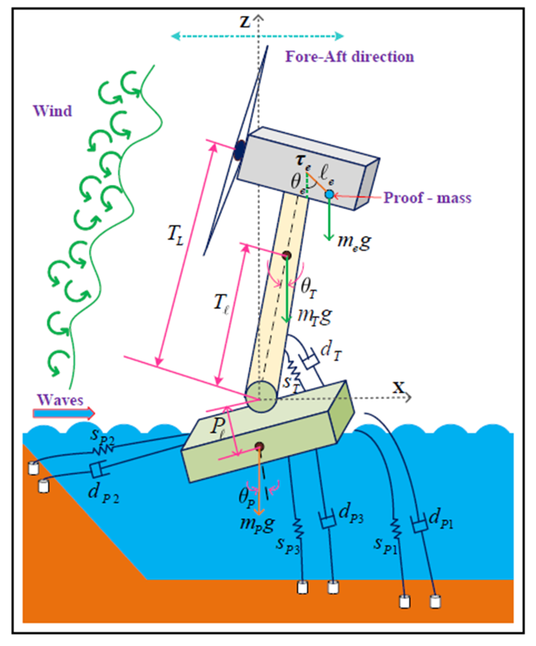
The barge-type TORA-based five degrees of freedom (5DOF) OFWT model has been taken from our recent research article [14], as shown in Figure 1. It is capable of generating five megawatts. Towards the direction of the negative z-axis, the rotating proof mass (18 m × 6 m × 6 m) has been attached outside of the nacelle. The hub height of the tower is 90 m. The dimension of the barge-type platform attached with mooring lines is (40 m × 40 m × 10 m). The overall OFWT vibratory motion has been considered a linear movement component of the TORA, whereas the proof mass circular motion represents the TORA controllable actuated component. In this way, the five degrees of freedom OFWT model has become an underactuated mechanical system. The designed dynamic system consists of proof-mass rotational movement, tower fore–aft bending, platform pitch motion, and two linear surge and heave displacements. In this research work, the generator’s dynamic behavior, degrees of freedom, rotor, and gearbox will not be used according to the designed model [13]. For the fore–aft and pitch motion of the tower and the platform, respectively, the approximated small-angle is used despite the most severe wave and wind cases, so that the equilibrium position not does exceed 10 degrees [5]. It is considered that the proof-mass actuator in the proposed OFWT is unable to cross 90 degrees out of its state of equilibrium due to the small-angle approximation.
Figure 1 presents a pivoting linear rigid beam with the same point of origin XYZ reference frame, where the pivot point connects the platform with the tower. The size from the middle of the platform to the middle of the mutual pivot point is denoted by P , and, respectively, the mass of the barge-type platform and its moment of inertia are denoted by m P and I P . The platform and tower’s attached dampers coefficient, d P 1 , d P 2 , d P 3 , d T , and the tightness of springs, S P 1 , S P 2 , S P 3 , S T , have constant values. Likewise, m T and I T , respectively, represent the mass of the tower and its moment of inertia. T L stands for the distance between the nacelle’s mid-point and the mutual pivot point, and T stands for the distance between the center of mass of the tower and the mutual pivot point. Gravity is denoted with g , and m e is the mass composed of the rotary proof mass m e 1 with the attached rod mass m e 2 . The rotating proof mass has a moment of inertia I e , where e stands for the rod size from the applicable control input τ e to the rotary proof mass. The angles θ e , θ T , θ P stand for angular positions and θ ˙ e , θ ˙ T , θ ˙ P stand for the angular velocities of the rotary proof mass, tower, and platform. The translational positions X P , Z P , and respective velocities are represented by X ˙ P , Z ˙ P .
After thoroughly examining and grasping the working theory of the TORA active mass damper control approach and using the OFWT system, the mathematical model of the TORA floating wind turbine has been obtained using the Euler–Lagrange equation of motion [14]. The following are some necessary equations taken from the derived model [14]. The overall kinetic energy of the considered model is determined by finding the platform kinetic energy K m P , tower kinetic energy K m T , and rotary proof-mass kinetic energy K m e , as follows:
K T = K m P + K m T + K m e = 1 2 I P θ ˙ P 2 + 1 2 I T θ ˙ T 2 + 1 2 I e θ ˙ e 2 + 1 2 m P ( X ˙ P 2 + Z ˙ P 2 ) + 1 2 m T X ˙ P + d d t T sin θ T 2 + Z ˙ P + d d t T cos θ T 2 + 1 2 m T X ˙ P + d d t T L sin θ T + d d t e sin θ e 2 + Z ˙ P + d d t T L cos θ T + d d t e cos θ e 2
In the same way, the overall potential energy of the considered model is determined by finding the platform potential energy U m P , tower potential energy U m T , and rotary proof-mass potential energy U m e , as follows:
U T = U m P + U m T + U m e = 1 2 s P 1 θ P 2 + 1 2 s P 2 X P 2 + 1 2 s P 3 Z P 2 m P g P cos θ P + 1 2 s T θ T θ P 2 + m T g T cos θ T + 1 2 s T θ T θ P 2 + m T g T cos θ T + m e g T L cos θ T e cos θ e
The Lagrangian of the system is determined by the difference between K T and U T   as follows:
L = K T U T = 1 2 ( I P θ ˙ P 2 + I T θ ˙ T 2 + I e θ ˙ e 2 ) + 1 2 m P ( X ˙ P 2 + Z ˙ P 2 ) + 1 2 m T X ˙ P 2 + 2 X ˙ P T cos θ T θ ˙ T + T 2 θ ˙ T 2 + Z ˙ P 2 2 Z ˙ P T sin θ T θ ˙ T 1 2 s P 1 θ P 2 + m P g P cos θ P 1 2 s T ( θ P 2 + θ T 2 2 θ P θ T ) m T g T cos θ T + 1 2 m e X ˙ P 2 + Z ˙ P 2 + T L 2 θ ˙ T 2 + e 2 θ ˙ e 2 + 2 T L θ ˙ T X ˙ P cos θ T Z ˙ e sin θ T + 2 e θ ˙ e X ˙ P cos θ e Z ˙ P sin θ e + 2 T L e θ ˙ T θ ˙ e cos θ T θ e m e g T L cos θ T e cos θ e 1 2 ( s P 2 X P 2 + s P 3 Z P 2 )
By using the Euler–Lagrange equations of motion, the respective dynamics of the barge-type TORA-based five degrees of freedom OFWT model are as follows:
m P + m T + m e X ¨ P + m e e cos θ e θ ¨ e + d P 2 X ˙ P + m T T cos θ T + m e T L cos θ T θ ¨ T m e e sin θ e θ ˙ e 2 m T T sin θ T + m e T L sin θ T θ ˙ T 2 + s P 2 X P = 0 m P + m T + m e Z ¨ P m e e sin θ e θ ¨ e + d P 3 Z ˙ P m T T sin θ T + m e T L sin θ T θ ¨ T m e e cos θ e θ ˙ e 2 m T T cos θ T + m e T L cos θ T θ ˙ T 2 + s P 3 Z P = 0 I P θ ¨ P + d T + d P 1 θ ˙ P d T θ ˙ T + s T + s P 1 θ P + m P g P sin θ P s T θ T = 0 I T + m T T 2 + m e T L 2 θ ¨ T + m e T L e cos θ T θ e θ ¨ e d T θ ˙ P + m T T cos θ T + m e T L cos θ T X ¨ P + d T θ ˙ T m T T sin θ T + m e T L sin θ T Z ¨ P s T θ P + s T θ T + m e T L e sin θ T θ e θ ˙ e 2 sin θ T m T g T + m e g T L = 0 I e + m e e 2 θ ¨ e + m e e cos θ e X ¨ P m e e sin θ e Z ¨ P + m e T L e cos θ T θ e θ ¨ T + m e g e sin θ e m e T L e sin θ T θ e θ ˙ T 2 = τ e
where the platform mass is m P   = 6,150,000 kg, the tower mass is m T = 347,460 kg, the nacelle mass is m n c   = 350,000 kg, the proof mass is m e 1   = 84,000 kg and the proof-mass rod mass is m e 2   = 42,000 kg. The tower and proof-mass rod length are respectively taken as T L = 90 m and e   = 6 m. In general, P   = −0.28 m, 0, T   = 64 m is the center of the mass. Consequently I e = 3,528,000 kg × m 2 ,   I T = 182,170,000 kg × m 2 , and I P = 169,450,000 kg × m 2 are the inertia of the rotary proof mass, tower, and platform, where g   = 9.81 m / s 2 is the gravity constant. The stiffness value of the springs is s P 1 = 14,171,000,000 N/m, s P 2 = s P 3   = 1,417,100,000 N/m and s T = 97,990,000,000 N/m, and d T = 2,103,200,000 N × s / m ,   d P 1 = 3,637,400,000 N × s / m , and d P 2 = d P 3 = 363,740,000 N × s / m are the values of the dampers coefficient. Due to the small angles of the tower and platform, we have considered the following approximation: s i n θ T = θ T ,   s i n θ P = θ P ,   c o s θ T = 1 , and c o s θ P = 1 . For simplicity, let the system’s states be x = X P   X ˙ P   Z P   Z ˙ P   θ P   θ ˙ P   θ T   θ ˙ T   θ e   θ ˙ e T = x j   x k   x l   x m   x n   x o   x p   x q   x r   x s T   hence, the barge-type 5DOF TORA-based OFWT model into a generalized affine form will be as follows:
x ˙ = n x + o x u e
Equation (5) contains the following data:
n x = x k n j ( x ) x m n l ( x ) x o n n ( x ) x q n p ( x ) x s n r ( x ) T o x = 0 o j ( x ) 0 o l ( x ) 0 o n ( x ) 0 o p ( x ) 0 o r ( x ) T u e = τ e
where
det ( M ) = c 5 c 0 2 c 6 c 9 c 0 2 c 7 2 c 0 c 1 2 c 9 + 2 c 0 c 1 c 3 c 7 c 0 c 2 2 c 9 c 0 c 3 2 c 6 + 2 c 0 c 2 c 4 c 7 c 0 c 4 2 c 6 + c 1 2 c 4 2 2 c 1 c 2 c 3 c 4 + c 2 2 c 3 2 > 0
n j ( x ) = n j det ( M ) , n l ( x ) = n l det ( M ) , n n ( x ) = n n det ( M ) , n p ( x ) = n p det ( M ) , n r ( x ) = n r det ( M ) , o j ( x ) = o j det ( M ) , o l ( x ) = o l det ( M ) , o n ( x ) = o n det ( M ) , o p ( x ) = o p det ( M ) , o r ( x ) = o r det ( M )
d 1 = s P 2 x j d P 2 x k + c 2 x q 2 + c 4 x s 2 d 2 = s P 3 x l d P 3 x m + c 1 x q 2 + c 3 x s 2 d 3 = s T + s P 1 + c 12 x n d T + d P 1 x o + s T x p + d T x q d 4 = s T x n + d T x o + c 13 s T x p d T x q c 8 x s 2 d 5 = c 8 x q 2 c 14 sin x r
n j = c 5 d 1 c 0 c 7 2 d 4 c 1 c 4 2 d 5 c 3 c 2 2 + d 1 c 6 c 4 2 + d 1 c 9 c 2 2 + d 5 c 1 c 2 c 4 + d 4 c 2 c 3 c 4 d 5 c 0 c 1 c 7 2 d 1 c 2 c 4 c 7 + d 2 c 1 c 2 c 9 d 2 c 1 c 4 c 7 d 2 c 2 c 3 c 7 + d 4 c 0 c 1 c 9 d 4 c 0 c 3 c 7 + d 5 c 0 c 3 c 6 + d 2 c 3 c 4 c 6 d 1 c 0 c 6 c 9 o j = c 5 c 2 2 c 3 + c 1 c 2 c 4 c 0 c 1 c 7 + c 0 c 3 c 6
n l = c 5 d 2 c 0 c 7 2 + d 4 c 2 c 3 2 + d 5 c 4 c 1 2 + d 2 c 6 c 3 2 + d 2 c 9 c 1 2 d 5 c 1 c 2 c 3 d 4 c 1 c 3 c 4 + d 1 c 1 c 2 c 9 d 1 c 1 c 4 c 7 d 1 c 2 c 3 c 7 2 d 2 c 1 c 3 c 7 + d 1 c 3 c 4 c 6 + d 5 c 0 c 2 c 7 d 4 c 0 c 2 c 9 + d 4 c 0 c 4 c 7 d 5 c 0 c 4 c 6 d 2 c 0 c 6 c 9 o l = c 5 c 1 2 c 4 c 1 c 2 c 3 + c 0 c 2 c 7 c 0 c 4 c 6
n n = d 3 c 0 2 c 7 2 c 6 c 9 c 0 2 + c 0 c 9 c 1 2 2 c 0 c 1 c 3 c 7 + c 0 c 9 c 2 2 2 c 0 c 2 c 4 c 7 + c 0 c 6 c 3 2 + c 0 c 6 c 4 2 c 1 2 c 4 2 + 2 c 1 c 2 c 3 c 4 c 2 2 c 3 2
n p = c 5 d 1 c 1 c 4 2 d 2 c 2 c 3 2 d 4 c 0 c 3 2 d 4 c 0 c 4 2 d 5 c 7 c 0 2 + d 4 c 9 c 0 2 + d 5 c 0 c 1 c 3 d 1 c 2 c 3 c 4 + d 2 c 1 c 3 c 4 d 1 c 0 c 1 c 9 + d 1 c 0 c 3 c 7 + d 5 c 0 c 2 c 4 + d 2 c 0 c 2 c 9 d 2 c 0 c 4 c 7 o p = d 5 c 7 c 0 2 + c 0 c 1 c 3 + c 0 c 2 c 4
n r = c 5 d 1 c 3 c 2 2 + d 5 c 0 c 1 2 + d 2 c 4 c 1 2 + d 5 c 0 c 2 2 + d 4 c 7 c 0 2 d 5 c 6 c 0 2 + d 1 c 1 c 2 c 4 d 2 c 1 c 2 c 3 d 4 c 0 c 1 c 3 d 1 c 0 c 1 c 7 + d 1 c 0 c 3 c 6 d 4 c 0 c 2 c 4 + d 2 c 0 c 2 c 7 d 2 c 0 c 4 c 6   o r = c 5 c 0 c 1 2 + c 0 c 2 2 c 6 c 0 2
where the equilibrium points of the 5DOF barge-type OFWT model are as follows:
x e q = 0 , 0 , 0 , 0 , 0 , 0 , 0 , 0 , θ e q , 0 T , θ e q = i π , i = 0 , ± 1 , ± 2 ,
We supposed that the nacelle’s rotary proof mass could not reach 90° from the equilibrium position due to the small-angle approximation. Therefore, the equilibrium position is θ e q = 0 in Equation (15). The robust adaptive control laws for the output constraints of the 5DOF barge-type TORA-based OFWT are developed in the following parts.

3. Design of Robust Adaptive ISMC Algorithm

The design of a robust control algorithm for the TORA actuator in a nacelle is required to reduce the overall system’s vibrations effectively. The dynamics of 5DOF barge-type TORA-based OFWT have nonlinearities that are subjected to a variety of perturbations caused by unknown disturbances and parametric uncertainties. We can take the following matched perturbation in a suggested generalized form of Equation (5), as follows:
x ˙ = n x + o x u e + Υ i t
where Υ i t is the matched perturbation and i = 1 , 2 , 3 , 4 , 5 . To implement the robust control technique [22], the general affine form of Equation (16) must be divided into second-order nonlinear systems. In this way, we will be able to achieve the following subsystems:
{ x ˙ j = x k x ˙ k = n j ( x ) + o j ( x ) u e + Υ 1 ( t ) x ˙ l = x m x ˙ m = n l ( x ) + o l ( x ) u e + Υ 2 ( t ) x ˙ n = x o x ˙ o = n n ( x ) + Υ 3 ( t ) x ˙ p = x q x ˙ q = n p ( x ) + o p ( x ) u e + Υ 4 ( t ) x ˙ r = x s x ˙ s = n r ( x ) + o r ( x ) u e + Υ 5 ( t )
where x j , x k , x l , x m , x n , x o , x p , x q , x r , x s are the state variables. A three-step method will be used to implement a robust adaptive control scheme for a rotary actuator of the proof mass. Firstly, by using the backstepping methodology, a backstepped OFWT subsystem model will be achieved. After this, we will design an adaptive chattering suppression gain for robust backstepping integral sliding mode control laws. Finally, we will design a high-gain observer with stability analysis for the suggested model. The backstepping procedure [30] has been adapted to convert the proposed model (17) to another pattern. For this, a new state variable is selected for the first subsystem of Equation (17) as follows:
μ 1 = x j
Next, we choose the Lyapunov function and take its derivative, as follows:
V ( μ 1 ) = 0.5 μ 1 2
V ˙ ( μ 1 ) = μ 1 μ ˙ 1 = μ 1 x k
Select a fictitious control input value x k to maintain the stability of μ 1 , as in:
x k = λ 1 μ 1
where λ 1 > 0 . Equation (20) is modified by substituting the value of x k , giving:
V ˙ ( μ 1 ) = λ 1 μ 1 2
By selecting μ 1 , stable λ 1 dynamics can be achieved. Equation (21) will be backstepped and the variable changed, such as:
μ 2 = x k + λ 1 μ 1
Following the aforementioned method, the chosen state variables of backstepping in a subsystem form of Equation (17) will be:
μ 1 = x j μ 2 = x k + λ 1 μ 1 μ 3 = x l μ 4 = x m + λ 2 μ 3 μ 5 = x n μ 6 = x o + λ 3 μ 5 μ 7 = x p μ 8 = x q + λ 4 μ 7 μ 9 = x k μ 10 = x s + λ 5 μ 9
where λ 2 , λ 3 , λ 4 , λ 5 represent the positive constants. The remaining Lyapunov functions are defined as V μ 3 = 0.5 μ 3 2 , V μ 5 = 0.5 μ 5 2 , V μ 7 = 0.5 μ 7 2 , V μ 9 = 0.5 μ 9 2 . The rest of the fictitious control inputs have been taken as: x m = λ 2 μ 3 ,   x o = λ 3 μ 5 ,     x q = λ 4 μ 7 ,   x s = λ 5 μ 9 . Taking the Equation (24) derivative and further evaluating it, the following results will be achieved:
μ ˙ 1 = μ 2 λ 1 μ 1 μ ˙ 2 = n j ( x ) + o j ( x ) u e + λ 1 ( μ 2 λ 1 μ 1 ) + Υ 1 ( t ) μ ˙ 3 = μ 4 λ 2 μ 3 μ ˙ 4 = n l ( x ) + o l ( x ) u e + λ 2 ( μ 4 λ 2 μ 3 ) + Υ 2 ( t ) μ ˙ 5 = μ 6 λ 3 μ 5 μ ˙ 6 = n n ( x ) + λ 3 ( μ 6 λ 3 μ 5 ) + Υ 3 ( t ) μ ˙ 7 = μ 8 λ 4 μ 7 μ ˙ 8 = n p ( x ) + o p ( x ) u e + λ 4 ( μ 8 λ 4 μ 7 ) + Υ 4 ( t ) μ ˙ 9 = μ 10 λ 5 μ 9 μ ˙ 10 = n r ( x ) + o r ( x ) u e + λ 5 ( μ 10 λ 5 μ 9 ) + Υ 5 ( t )
The second-order backstepping-based subsystems of the presented OFWT system are represented by Equation (25). Furthermore, two different control algorithms are presented for the stabilization of the OFWT model. The first one is called an adaptive integral sliding mode control and the second is the adaptive integral sliding mode control using BLF. The sliding manifold for each subsystem of Equation (25) is used for designing proposed control laws, as follows:
σ 1 = σ a + σ a d t
σ 2 = σ b + σ b d t
σ 3 = σ c + σ c d t
σ 4 = σ d + σ d d t
σ 5 = σ e + σ e d t
where σ a = α 1 μ 1 + μ 2 ,     σ b = α 2 μ 3 + μ 4 ,   σ c = α 3 μ 5 + μ 6 ,   σ d = α 4 μ 7 + μ 8 ,   σ e = α 5 μ 9 + μ 10 , and α 1 , α 2 , α 3 , α 4 , α 5 are the positive constants. The surfaces (26)–(30) sum and respective derivatives sum are as follows:
σ T = σ 1 + σ 2 + σ 3 + σ 4 + σ 5
where
σ ˙ 1 = α 1 μ 1 ( 1 λ 1 ) + μ 2 ( α 1 + 1 ) + λ 1 ( μ 2 λ 1 μ 1 ) + n j ( x ) + o j ( x ) u e + ϒ 1 ( t )
σ ˙ 2 = α 2 μ 3 ( 1 λ 2 ) + μ 4 ( α 2 + 1 ) + λ 2 ( μ 4 λ 2 μ 3 ) + n l ( x ) + o l ( x ) u e + ϒ 2 ( t )
σ ˙ 3 = α 3 μ 5 ( 1 λ 3 ) + μ 6 ( α 3 + 1 ) + λ 3 ( μ 6 λ 3 μ 5 ) + n n ( x ) + ϒ 3 ( t )
σ ˙ 4 = α 4 μ 7 ( 1 λ 4 ) + μ 8 ( α 4 + 1 ) + λ 4 ( μ 8 λ 4 μ 7 ) + n p ( x ) + o p ( x ) u e + ϒ 4 ( t )
σ ˙ 5 = α 5 μ 9 ( 1 λ 5 ) + μ 10 ( α 5 + 1 ) + λ 5 ( μ 10 λ 5 μ 9 ) + n r ( x ) + o r ( x ) u e + ϒ 5 ( t )
Theorem 1.
Consider the backstepping-based proposed model (25) and select the sliding manifold as in Equation (31) for the adaptive ISMC algorithm, as follows:
u e = ( o j ( x ) + o l ( x ) + o p ( x ) + o r ( x ) ) 1 [ α 1 μ 1 ( 1 λ 1 ) + μ 2 ( α 1 + 1 ) + λ 1 ( μ 2 λ 1 μ 1 ) + n j ( x ) + α 2 μ 3 ( 1 λ 2 ) + μ 4 ( α 2 + 1 ) + λ 2 ( μ 4 λ 2 μ 3 ) + n l ( x ) + α 3 μ 5 ( 1 λ 3 ) + μ 6 ( α 3 + 1 ) + λ 3 ( μ 6 λ 3 μ 5 ) + n n ( x ) + α 4 μ 7 ( 1 λ 4 ) + μ 8 ( α 4 + 1 ) + n p ( x ) + λ 4 ( μ 8 λ 4 μ 7 ) + α 5 μ 9 ( 1 λ 5 ) + μ 10 ( α 5 + 1 ) + λ 5 ( μ 10 λ 5 μ 9 ) + n r ( x ) + κ ^ ( t ) σ T + Ω T s i g n ( σ T ) ]
where the adaptive gain is represented by κ ^ T t and switching gain is represented by Ω T > 0 . The proposed control algorithm will effectively stabilize the OFWT, against all the matched unknown bounded perturbations.
Proof of Theorem 1.
Stability analysis using the Lyapunov function is a very precise method of control design. We took a Lyapunov candidate function, such as:
V T = 0.5 ( σ T 2 + η 1 κ ˜ T 2 ( t ) )
where κ ˜ T t = κ T κ ^ T t ,   κ ˜ ˙ T t = κ ^ ˙ T t , and κ T ,   η are the bounded positive constants. Now, substituting the respective values after taking the derivative of the Lyapunov function (38) to time yields:
V ˙ T = σ T σ ˙ T + η 1 κ ˜ T ( t ) κ ˜ ˙ T ( t ) = σ T [ α 1 μ 1 ( 1 λ 1 ) + μ 2 ( α 1 + 1 ) + λ 1 ( μ 2 λ 1 μ 1 ) + n j ( x ) + Υ 1 ( x , t ) + α 2 μ 3 ( 1 λ 2 ) + μ 4 ( α 2 + 1 ) + λ 2 ( μ 4 λ 2 μ 3 ) + n l ( x ) + Υ 2 ( x , t ) + α 3 μ 5 ( 1 λ 3 ) + μ 6 ( α 3 + 1 ) + λ 3 ( μ 6 λ 3 μ 5 ) + n n ( x ) + Υ 3 ( x , t ) + α 4 μ 7 ( 1 λ 4 ) + μ 8 ( α 4 + 1 ) + n p ( x ) + Υ 4 ( x , t ) + λ 4 ( μ 8 λ 4 μ 7 ) + α 5 μ 9 ( 1 λ 5 ) + μ 10 ( α 5 + 1 ) + λ 5 ( μ 10 λ 5 μ 9 ) + n r ( x ) + Υ 5 ( x , t ) + ( o j ( x ) + o l ( x ) + o p ( x ) + o r ( x ) ) u e ] η 1 κ ˜ T ( t ) κ ^ ˙ T ( t )
Now, substituting the control input u e into Equation (39) yields:
V ˙ T = σ T Υ 1 ( t ) + Υ 2 ( t ) + Υ 3 ( t ) + Υ 4 ( t ) + Υ 5 ( t ) Ω T σ T κ ^ T ( t ) σ T 2 η 1 κ ˜ T ( t ) κ ^ ˙ T ( t ) + κ T σ T 2 κ T σ T 2 = σ T Υ 1 ( t ) + Υ 2 ( t ) + Υ 3 ( t ) + Υ 4 ( t ) + Υ 5 ( t ) Ω T σ T + κ ˜ T ( t ) σ T 2 η 1 κ ˜ T ( t ) κ ^ ˙ T ( t ) κ T σ T 2 = σ T Υ 1 ( t ) + Υ 2 ( t ) + Υ 3 ( t ) + Υ 4 ( t ) + Υ 5 ( t ) Ω T σ T κ T σ T 2 + κ ˜ T ( t ) ( σ T 2 η 1 κ ^ ˙ T ( t ) )
where the adaptive gain is designed from κ ^ ˙ T t = η σ T 2 . Let β > 0 and fulfils the bounded unknown perturbation constraint as Υ 1 t β 1 ,   Υ 2 t β 2 ,   Υ 3 t β 3 ,   Υ 4 t β 4 ,   Υ 5 t β 5 where β = β 1 + β 2 + β 3 + β 4 + β 5 . After applying these parameter values, Equation (40) will be as follows:
V ˙ T σ T [ Ω T β ] κ T σ T 2
where Ω T = β + ψ ,   ψ > 0 , and further simplifying yields:
V ˙ T ψ σ T κ T σ T 2
The derivative of the Lyapunov function is negative definite, as shown in Equation (42). As a result, the suggested control algorithm stabilizes the system effectively and robustly, completing the verification. □
Theorem 2.
Consider the backstepping-based proposed model (25) and select the sliding manifold as in Equation (31) for adaptive ISMC algorithm with output constraint ( μ 5 ω 0 and μ 7 ω 1 ), as follows:
u e = ( o j ( x ) + o l ( x ) + o p ( x ) + o r ( x ) ) 1 [ α 1 μ 1 ( 1 λ 1 ) + μ 2 ( α 1 + 1 ) + λ 1 ( μ 2 λ 1 μ 1 ) + n j ( x ) + α 2 μ 3 ( 1 λ 2 ) + μ 4 ( α 2 + 1 ) + λ 2 ( μ 4 λ 2 μ 3 ) + n l ( x ) + α 3 μ 5 ( 1 λ 3 ) + μ 6 ( α 3 + 1 ) + λ 3 ( μ 6 λ 3 μ 5 ) + n n ( x ) + α 4 μ 7 ( 1 λ 4 ) + μ 8 ( α 4 + 1 ) + n p ( x ) + λ 4 ( μ 8 λ 4 μ 7 ) + α 5 μ 9 ( 1 λ 5 ) + μ 10 ( α 5 + 1 ) + λ 5 ( μ 10 λ 5 μ 9 ) + n r ( x ) + κ ^ ( t ) σ T + ( ω 0 2 μ 5 2 ) 1 ( ν 0 μ 5 σ 3 ) + ( ω 1 2 μ 7 2 ) 1 ( ν 1 μ 7 σ 4 ) + Ω T ( ( ω 0 2 μ 5 2 ) 0.5 ( μ 5 ) + ( ω 1 2 μ 7 2 ) 0.5 ( μ 7 ) + ( | 2 σ T | ) 0.5 ) s i g n ( σ T ) ψ 1 s i g n ( σ T ) ψ 2 s i g n ( σ T ) ]
where   ν 0 ,   ν 1 ,   ω 0 ,   ω 1 are the positive gains, the adaptive and switching gains are respectively as:  κ ^ T t ,   Ω T > 0 . The proposed control algorithm will effectively stabilize the OFWT to the output constraint, against all the matched unknown bounded perturbations.
Proof of Theorem  2.
Select a Lyapunov candidate function, as follows:
V T = σ T + 0.5 ( ν 0 ln ( ( ω 0 2 μ 5 2 ) 1 ( ω 0 2 ) ) + ν 1 ln ( ( ω 1 2 μ 7 2 ) 1 ( ω 1 2 ) ) + η 1 κ ˜ T 2 ( t ) )
where κ ˜ T t = κ T κ ^ T t ,     κ ˜ ˙ T t = κ ^ ˙ T t ,   κ T > 0 , and η > 0 . Now, substituting the respective values after taking the derivative of the Lyapunov function (44) to time yields:
V ˙ T = σ ˙ T s i g n ( σ T ) + ( ( ω 0 2 μ 5 2 ) 1 ( ν 0 μ 5 μ ˙ 5 ) ) + ( ( ω 1 2 μ 7 2 ) 1 ( ν 1 μ 7 μ ˙ 7 ) ) η 1 κ ˜ T ( t ) κ ^ ˙ T ( t )
V ˙ T = s i g n ( σ T ) [ α 1 μ 1 ( 1 λ 1 ) + μ 2 ( α 1 + 1 ) + λ 1 ( μ 2 λ 1 μ 1 ) + n j ( x ) + Υ 1 ( t ) + α 2 μ 3 ( 1 λ 2 ) + μ 4 ( α 2 + 1 ) + λ 2 ( μ 4 λ 2 μ 3 ) + n l ( x ) + α 3 μ 5 ( 1 λ 3 ) + Υ 2 ( t ) + μ 6 ( α 3 + 1 ) + λ 3 ( μ 6 λ 3 μ 5 ) + n n ( x ) + Υ 3 ( t ) + α 4 μ 7 ( 1 λ 4 ) + μ 8 ( α 4 + 1 ) + n p ( x ) + Υ 4 ( t ) + λ 4 ( μ 8 λ 4 μ 7 ) + α 5 μ 9 ( 1 λ 5 ) + μ 10 ( α 5 + 1 ) + λ 5 ( μ 10 λ 5 μ 9 ) + n r ( x ) + Υ 5 ( t ) + ( ω 0 2 μ 5 2 ) 1 ( ν 0 μ 5 σ 3 ) + ( ω 1 2 μ 7 2 ) 1 ( ν 1 μ 7 σ 4 ) + ( o j ( x ) + o l ( x ) + o p ( x ) + o r ( x ) ) u e ] ψ 1 ψ 2 ψ 3 ψ 4 η 1 κ ˜ T ( t ) κ ^ ˙ T ( t )
where the following parameters are defined as ψ 1 = ω 0 2 μ 5 2 1 ν 0 μ 5 α 3 μ 5 + α 3 μ 5 d t + μ 6 d t   ,     ψ 3 =   ω 0 2 μ 5 2 1 ν 0 λ 3 μ 5 2   ,   ψ 2 = ω 1 2 μ 7 2 1   ν 1 μ 7   α 4 μ 7 + α 4 μ 7 d t + μ 8 d t ,   and   ψ 4 = ω 1 2 μ 7 2 1 ν 1 λ 4 μ 7 2 . Let β > 0 and fulfill the bounded unknown perturbation constraint as Υ 1 t β 1 ,   Υ 2 t β 2 ,   Υ 3 t β 3 ,   Υ 4 t β 4 ,   Υ 5 t β 5 , where β = β 1 + β 2 + β 3 + β 4 + β 5 . Now, substituting the control input u e in Equation (46) yields:
V ˙ T = Υ 1 ( t ) + Υ 2 ( t ) + Υ 3 ( t ) + Υ 4 ( t ) + Υ 5 ( t ) s i g n ( σ T ) Ω T ( ( ω 0 2 μ 5 2 ) 0.5 ( μ 5 2 ) 0.5 + ( ω 1 2 μ 7 2 ) 0.5 ( μ 7 2 ) 0.5 + ( | 2 σ T | ) 0.5 ) + κ T ( t ) σ T κ ^ T ( t ) σ T η 1 κ ˜ T ( t ) κ ^ ˙ T ( t ) κ T ( t ) σ T κ T ( t ) σ T + β s i g n ( σ T ) Ω T ( ln ( ω 0 2 μ 5 2 ) 0.5 ( ω 0 2 ) 0.5 + ln ( ω 1 2 μ 7 2 ) 0.5 ( ω 1 2 ) 0.5 + ( | 2 σ T | ) 0.5 ) + κ ˜ T ( t ) σ T η 1 κ ˜ T ( t ) κ ^ ˙ T ( t ) Ω T 2 V T
where the adaptive gain is designed from κ ^ ˙ T t = η σ T . The derivative of the Lyapunov function is negative definite, as shown in Equation (47). As a result, the suggested control algorithm stabilizes the system effectively and robustly, and will never become unbounded due to the conditions mentioned in Theorem 2. It completes the verification. □

4. Formulation of HGO

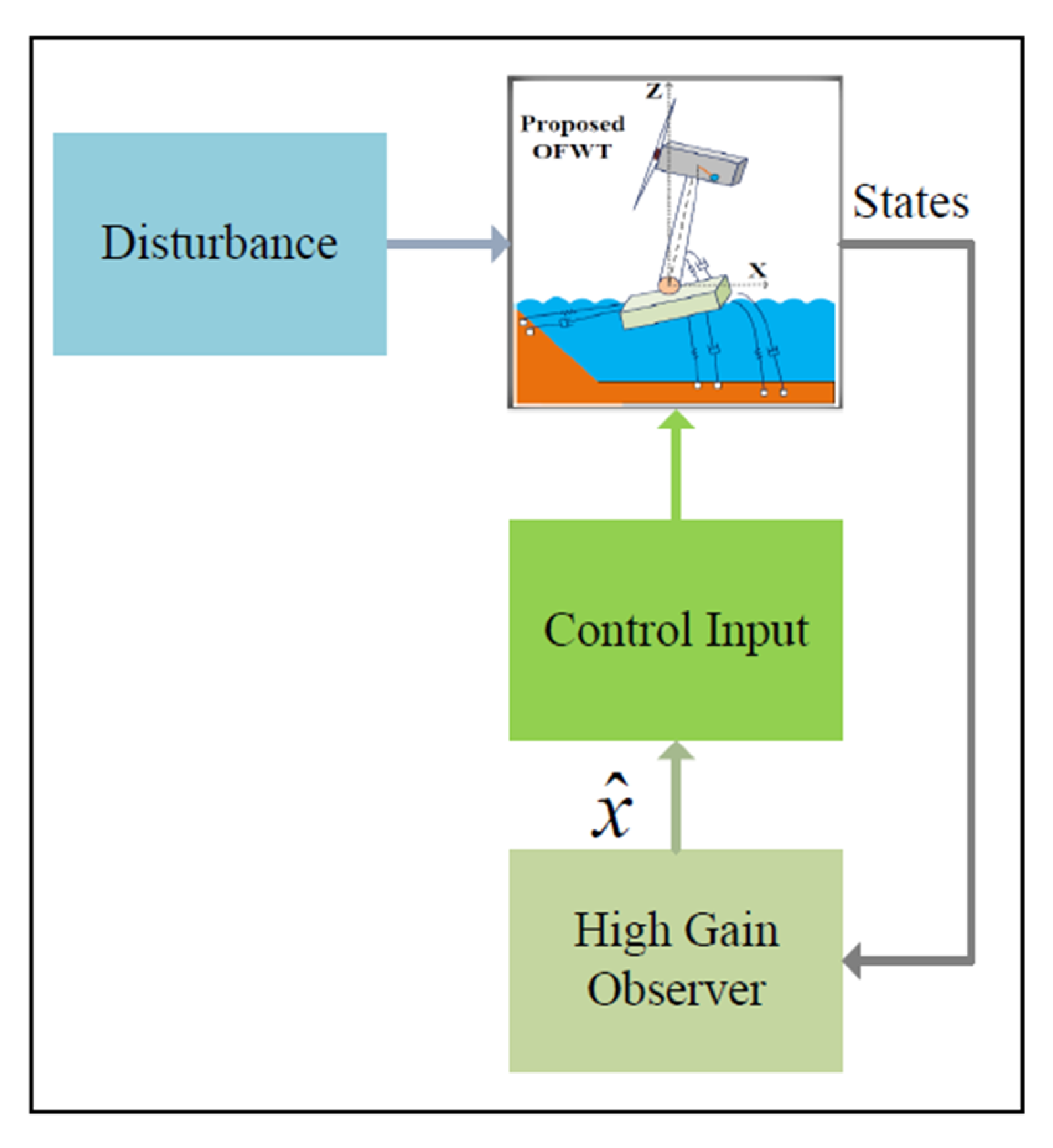
With information on desired output states, the high-gain observer can generate the estimation of the unknown states in the presence of system uncertainties and disturbances. The HGO’s state estimation property ensures that the controller has access to unknown states. Figure 2 represents the schematic diagram of the adaptive robust control scheme for the OFWT system. The HGO uses the actual system states information and provides all known and unknown estimated states to the control input of the closed-loop system, as shown in the schematic diagram.
In the form of a second order, we have presented five subsystems in this article, where each of them is defined in normal form. After that we developed HGOs for each subsystem for the nominal values of the system, as follows:
x ^ ˙ j = x ^ k + γ 1 ( x j x ^ j ) x ^ ˙ k = ϕ j ( x ^ , u ) + γ 2 ( x j x ^ j )
x ^ ˙ l = x ^ m + γ 3 ( x l x ^ l ) x ^ ˙ m = ϕ l ( x ^ , u ) + γ 4 ( x l x ^ l )
x ^ ˙ n = x ^ o + γ 5 ( x n x ^ n ) x ^ ˙ o = ϕ n ( x ^ , u ) + γ 6 ( x n x ^ n )
x ^ ˙ p = x ^ q + γ 7 ( x p x ^ p ) x ^ ˙ q = ϕ p ( x ^ , u ) + γ 8 ( x p x ^ p )
x ^ ˙ r = x ^ s + γ 9 ( x r x ^ r ) x ^ ˙ s = ϕ r ( x ^ , u ) + γ 10 ( x r x ^ r )
where ϕ j x ^ , u = n ^ j x + o ^ j x u e ,     ϕ l x ^ , u = n ^ l x + o ^ l x u e ,   ϕ n x ^ , u = n ^ n x ,   ϕ p x ^ , u = n ^ p x + o ^ p x u e , ϕ r x ^ , u = n ^ r x + o ^ r x u e ,   and γ 1 = a 1 1 / b ,   γ 2 = a 2 1 / b 2 ,   γ 3 = a 1 2 / b ,   γ 4 = a 2 2 / b 2 ,   γ 5 = a 1 3 / b ,   γ 6 = a 2 3 / b 2 ,   γ 7 = a 1 4 / b ,   γ 8 = a 2 4 / b 2 ,   γ 9 = a 1 5 / b ,   γ 10 = a 2 5 / b 2 ,   while b has a small positive constant value, such as b 1 . Constant parameters a 1 1 ,     a 2 1 ,     a 1 2 ,     a 2 2 ,     a 1 3 ,     a 2 3 ,   a 1 4 ,   a 2 4 , a 1 5 ,   a 2 5 are chosen from these polynomials s 2 + a 1 1 s + a 2 1 = 0 ,   s 2 + a 1 2 s + a 2 2 = 0 ,   s 2 + a 1 3 s + a 2 3 = 0 ,   s 2 + a 1 4 s + a 2 4 = 0 , and s 2 + a 1 5 s + a 2 5 = 0 in such a way that in the left half-plane, the polynomials’ roots will exist.
Stability Analysis: The stability analysis of the high-gain observer of the suggested barge-type OFWT model is determined by rewriting Equation (16) into a generalized form as follows:
x ˙ = A x + B ϕ ( x , u ) y = C x
where x R ρ ,   ρ = 10 ,   y R m ,   m = 5 ,   : R 5 × R R   is a real-valued map, and x , u   is the image of x , u . Overall, the proposed OFWT model Equation (16) has a 10-degree order ρ = 10 and each subsystem of the proposed OFWT model Equation (17) has a 2-degree order ρ = i = 1 5 ρ i . According to the HGO design [35], the derivative of estimated states can be expressed as follows:
x ^ ˙ = A x ^ + B ϕ ( x ^ , u ) + H C ( y x ^ )
where
x ˜ = x ˜ 1 x ˜ 2 x ˜ 3 x ˜ 4 x ˜ 5 x ˜ 6 x ˜ 7 x ˜ 8 x ˜ 9 x ˜ 10 = x 1 x ^ 1 x 2 x ^ 2 x 3 x ^ 3 x 4 x ^ 4 x 5 x ^ 5 x 6 x ^ 6 x 7 x ^ 7 x 8 x ^ 8 x 9 x ^ 9 x 10 x ^ 10
here, x ˜ is the estimation error of the observer. For simplicity, a notation can be defined as ξ x , x ^ = ϕ x , u ϕ x ^ , u . Now, taking the derivative of Equation (55) yields:
x ˜ ˙ = A 0 x ˜ + B 0 ξ ( x , x ^ )
where ξ x , x ^ = ξ 1 x , x ^   ξ 2 x , x ^   ξ 3 x , x ^   ξ 4 x , x ^   ξ 5 x , x ^ T . Now, the scale estimation is defined as ϖ i j = x i j x ^ i j / b ρ i j , where 1 i 5 and 1 j ρ j . After substituting the values, the scale estimation of each state is as follows: ϖ 11 = x ˜ 11 / b ,   ϖ 12 = x ˜ 12 . For simplicity, we assumed that ϖ 11 = x ˜ 11 / b = x ˜ 1 / b = ϖ 1 ,   ϖ 12 = x ˜ 12 = x ˜ 2 = ϖ 2 and similarly for the remaining parameters. From this, we can get b ϖ ˙ 1 = a 1 1 ϖ 1 + ϖ 2 ,   b ϖ ˙ 2 = a 2 1 ϖ 1 + b ξ 1 x , x ^ ,     ϖ 3 = x ˜ 3 / b ,     ϖ 4 = x ˜ 4 ,     ϖ 5 = x ˜ 5 / b ,   ϖ 6 = x ˜ 6 ,   ϖ 7 = x ˜ 7 / b ,   ϖ 8 = x ˜ 8 ,   ϖ 9 = x ˜ 9 / b ,   ϖ 10 = x ˜ 10 .   From the scale estimation of each state, a generalized form can be written as follows:
D ( b ) ϖ = x x ^
taking the derivative of Equation (57) and substituting the values yields:
ϖ ˙ = D 1 ( b ) ( A H C ) D ( b ) ϖ + D 1 ( b ) B ξ ( x , z , D ( b ) ϖ )
ϖ ˙ = b 1 ζ ϖ + B ξ ( x , z , D ( b ) ϖ )
hence, Equation (59) can be written as:
b ϖ ˙ = ζ ϖ + b B ξ ( x , z , D ( b ) ϖ )
since ζ is Hurwitz, thus it is concluded from Equation (60) that as the value b approaches zero, the uncertain term becomes zero, and the error converges to zero asymptotically. The derived matrices for the stability analysis are presented in Appendix A.

5. Simulation Results and Discussion

In this paper, MATLAB/SIMULINK software is utilized to simulate the mathematical model of the barge-type TORA-based 5DOF OFWT and as well as to verify the efficiency of the designed BLF-based adaptive backstepping ISMC compared with the adaptive backstepping ISMC law. As in the control design portion, we have selected a backstepping ISMC surface and designed two robust adaptive ISMC laws based on the high-gain observer. The objective of this study is to examine the OFWT model stability under the applied output constraints and to improve its performance in terms of stability by using the suggested control strategy. For this, the parametric values discussed in the suggested perturbed 5DOF OFWT model section have been used in simulation with the assumption that the system is in vibrating condition with these initial values:   x j 0 = 0.2 ,   x k 0 = 0 ,   x l 0 = 0.15 ,   x m 0 = 0 ,   x n 0 = π / 36 ,   x o 0 = 0 ,   x p 0 = π / 36 ,   x q 0 = 0 ,   x r 0 = 0 ,   x s 0 = 0 ,   where the following are the initial design conditions for the HGO: x ^ j 0 = 0 ,   x ^ k 0 = 0 ,   x ^ l 0 = 0 ,   x ^ m 0 = 0 ,   x ^ n 0 = 0 ,   x ^ o 0 = 0 ,   x ^ p 0 = 0 ,   x ^ q 0 = 0 ,   x ^ r 0 = 0 ,   and x ^ s 0 = 0 .
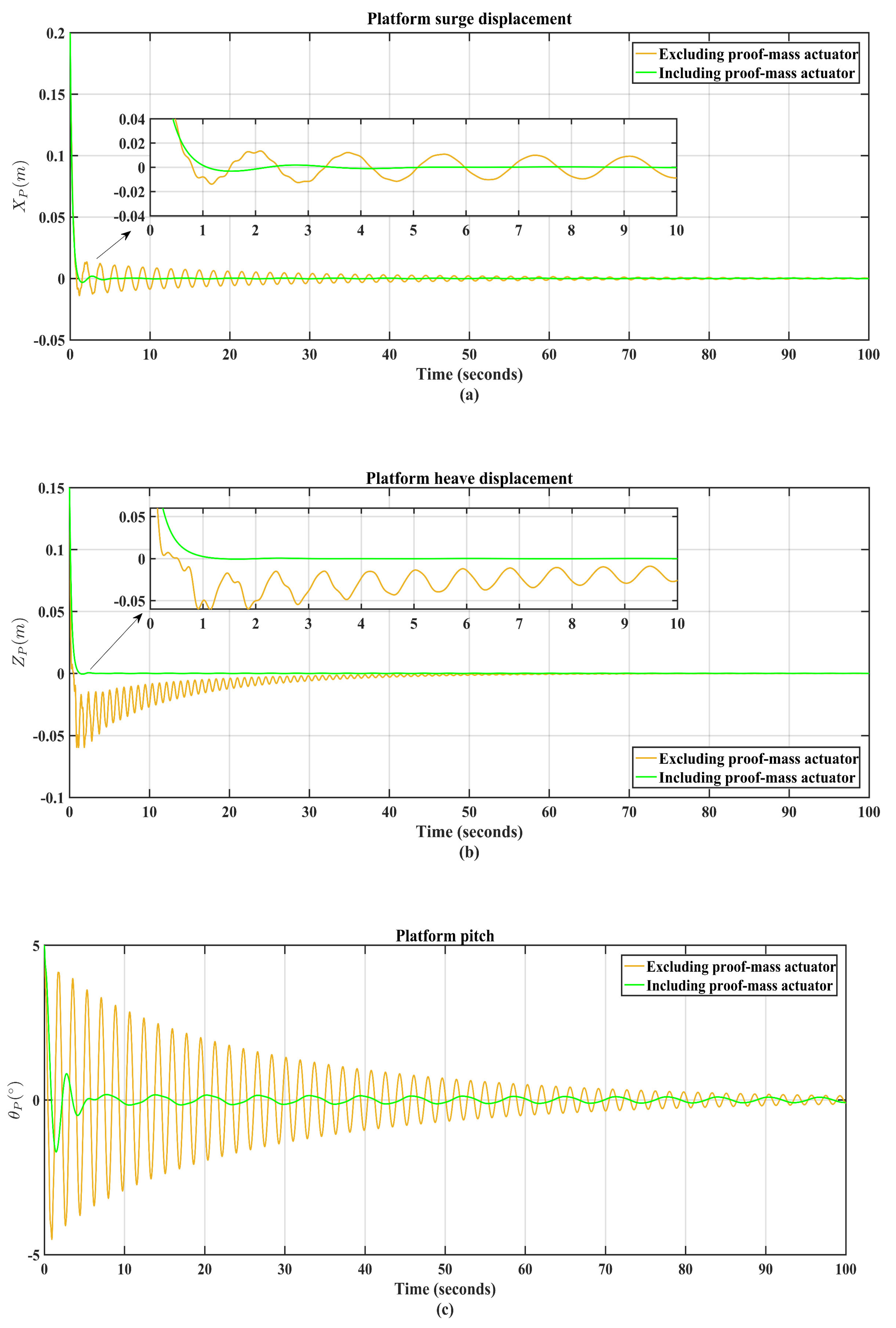
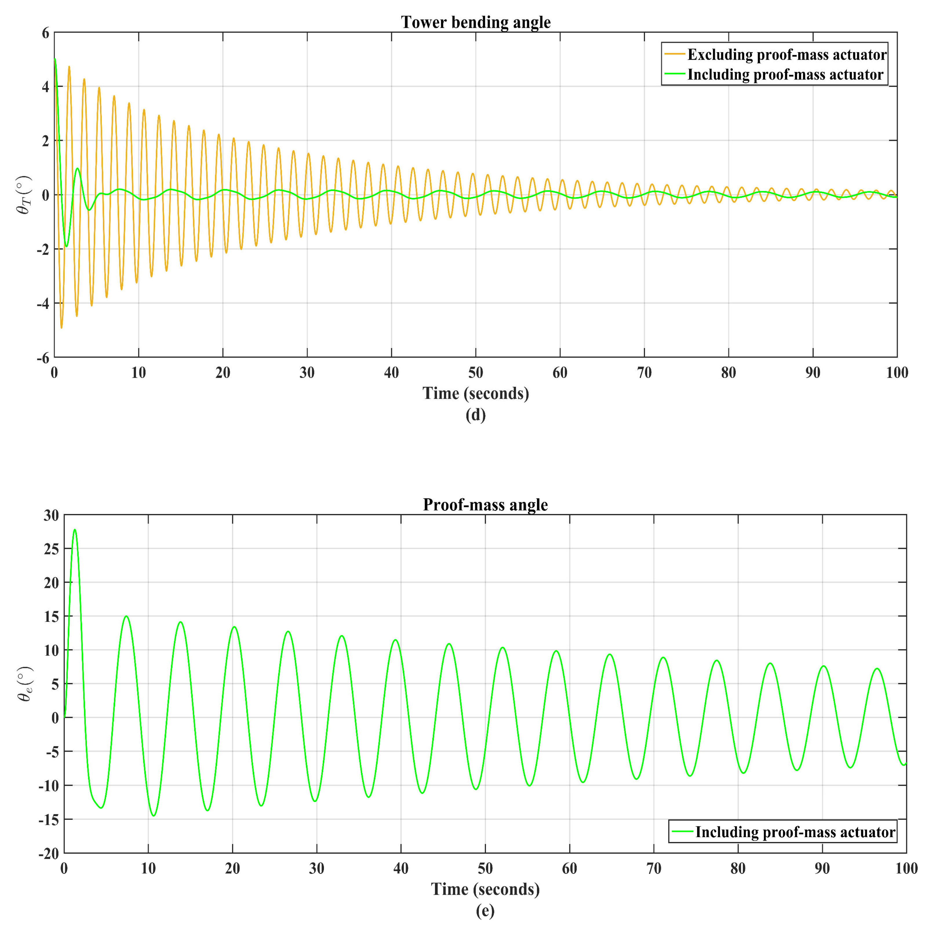
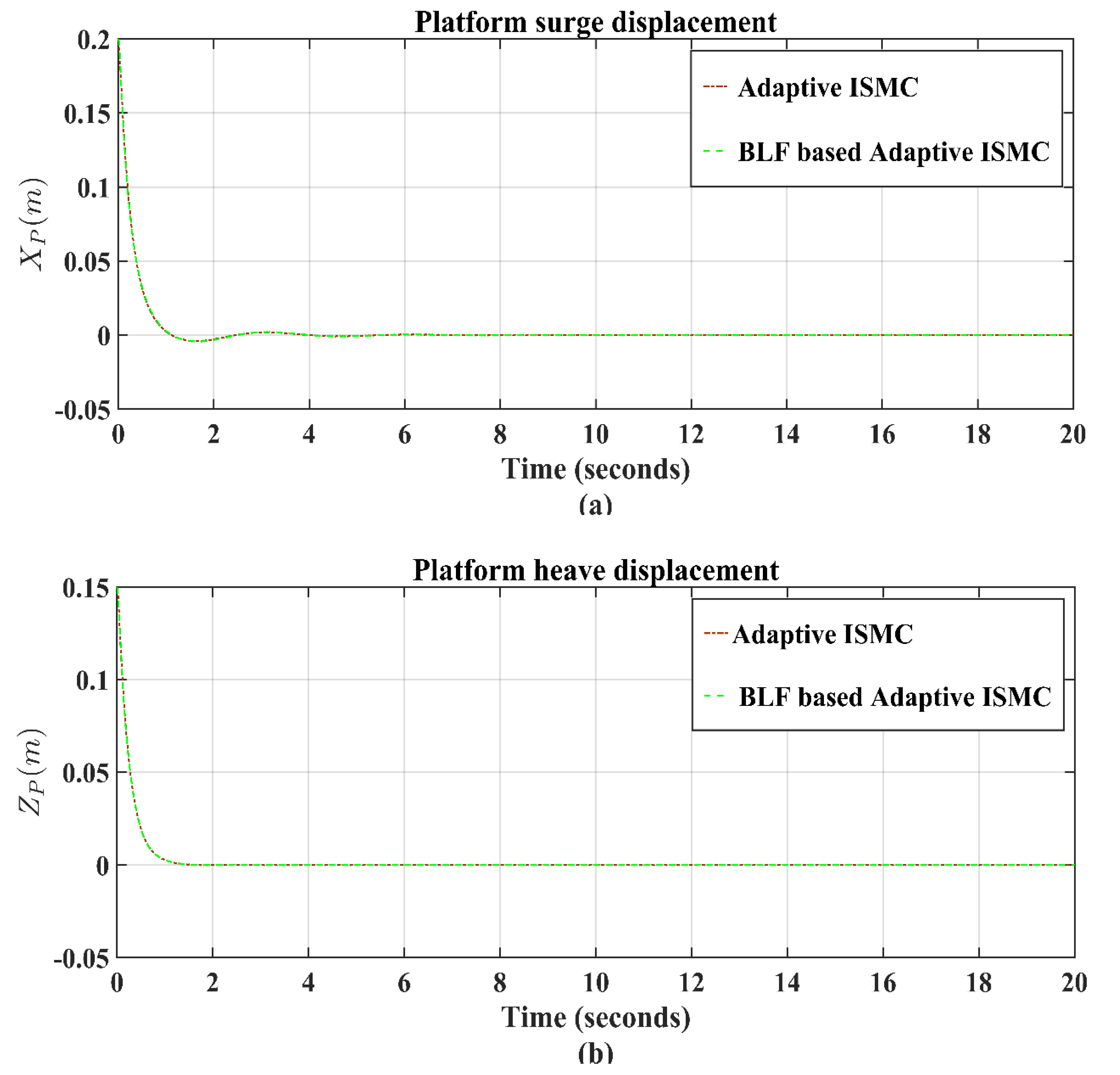
We have been able to achieve the simulation results displayed in Figure 3 by utilizing the initial values rather than incorporating control input. Throughout every simulation outcome,
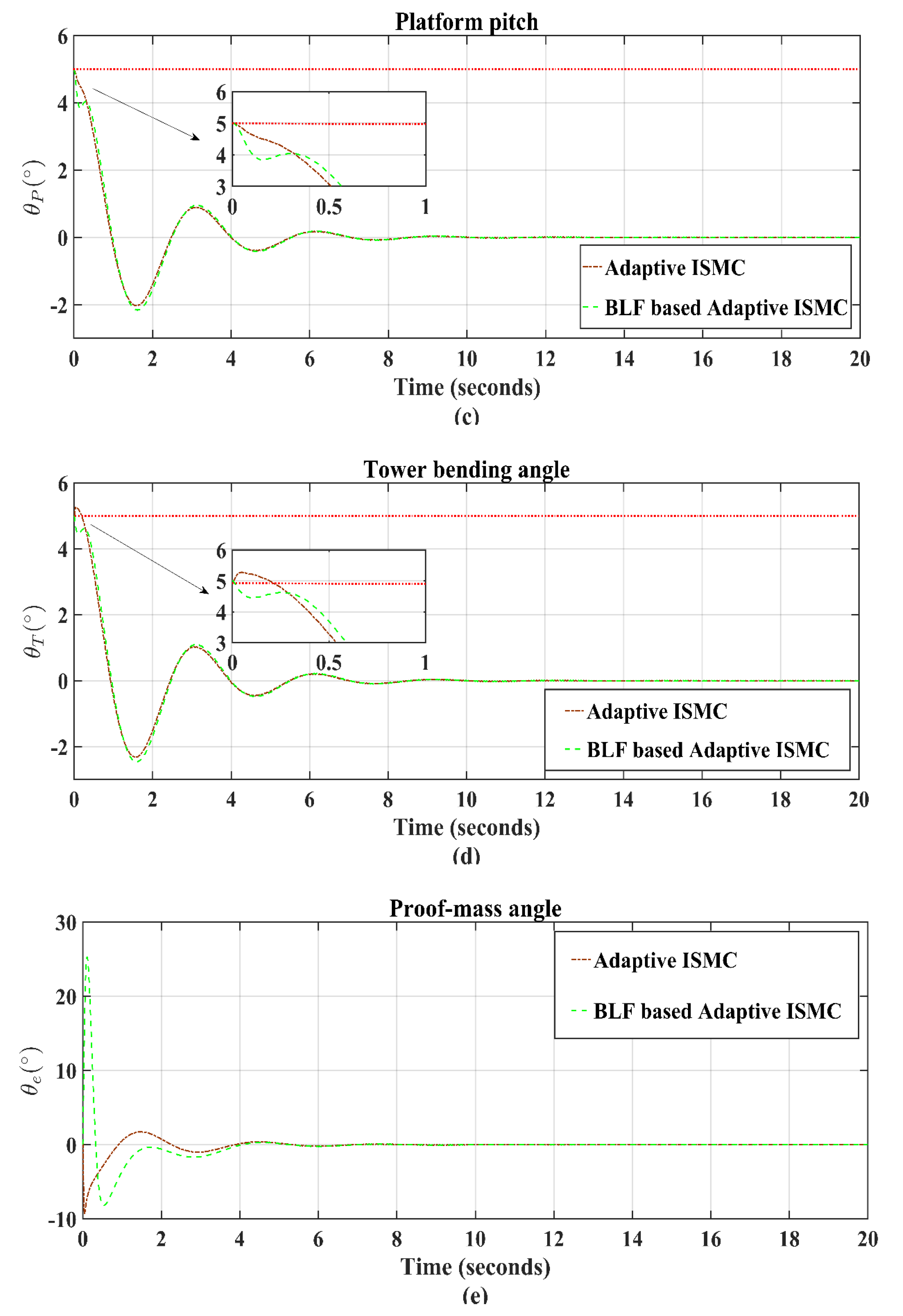
 X P of the part (a) and Z P of the part (b) represent the platform surge and heave linear displacement, while parts (c), (d), and (e) represent the platform pitch angle ( θ P ), bending tower angle ( θ T ), and rotary angle ( θ e ) of the TORA actuator, respectively. Without applying control laws, the suggested model’s natural response, including and excluding the actuated proof mass, has been studied using the system comparison analysis shown in Figure 3. Figure 3 shows that while achieving the equilibrium position, the effect of the vibration is smaller in the suggested proof-mass actuator model case, while Figure 3e shows the actuated proof-mass vibrating behavior. Similarly, without considering the actuated proof-mass case, Figure 3a,b go to their equilibrium position approximately in 60 s, while in the case of including the proof-mass actuator, and with no applying control input, the states go to the equilibrium position within 5 s. In the remaining subparts of Figure 3c–e, in both cases (excluding and including the proof-mass actuator model), the states go to their equilibrium position after 100 s, but the difference is in terms of vibrational amplitude. Furthermore, the barge-type OFWT is a fundamentally stable system, as has been demonstrated in the literature [6,9]. Our proposed model’s simulated results demonstrate a similar pattern to that shown in previous articles. As the standard matched sinusoidal disturbance, Υ i (t) is taken in our proposed model as a perturbation factor. The selection of disturbances Υ 1 (t) and Υ 2 (t) are used in such a way as to cause the drifting phenomena into the barge platform of the proposed model, where Υ 1 (t) = 5sin(2 π f t ) c o s φ s i n φ ,   Υ 2 (t) = 5sin(2 π f t ) s i n φ + c o s φ , and φ is the drifting angle. Moreover, Υ i (t) = 5sin(2 π f t ), i = 3 , 4 , 5 ,   f = 15   Hz , and φ = 30°.
The comparison study has been conducted by applying the proposed adaptive backstepping ISMC and BLF-based adaptive backstepping ISMC to the proof-mass actuator, as shown in Figure 4. Table 1 shows the positive constants parameters. For comparison purposes, we have chosen the same values for both tuning control laws. All the parts of Figure 4 show that the states go to their equilibrium position at the same time (within 10 s) by using the adaptive backstepping ISMC and the BLF-based adaptive backstepping ISMC. Parts (c) and (d) of Figure 4 show that the BLF-based control algorithm works accurately and bound the platform pitch angle and the tower bending angle within five degrees, while the adaptive backstepping ISMC violates the constraint. Furthermore, the proposed BLF-based adaptive backstepping ISMC better stabilizes the pitch and the bending movement of the barge-type OFWT tower within 10 s as compared with the active and passive control approaches mentioned in other articles [9,13]. Table 2 presents the root mean square error (RMSE) of Figure 4. For quantitative comparison purposes, Table 2 also presents the transient state and steady-state error response. From Table 2, it can be seen clearly that the error of controlled states (CS) using the adaptive backstepping ISMC and BLF-based adaptive backstepping ISMC shows a very small error. Overall, the RMSE of the controlled states using the adaptive backstepping ISMC has less error than the BLF-based adaptive backstepping ISMC.
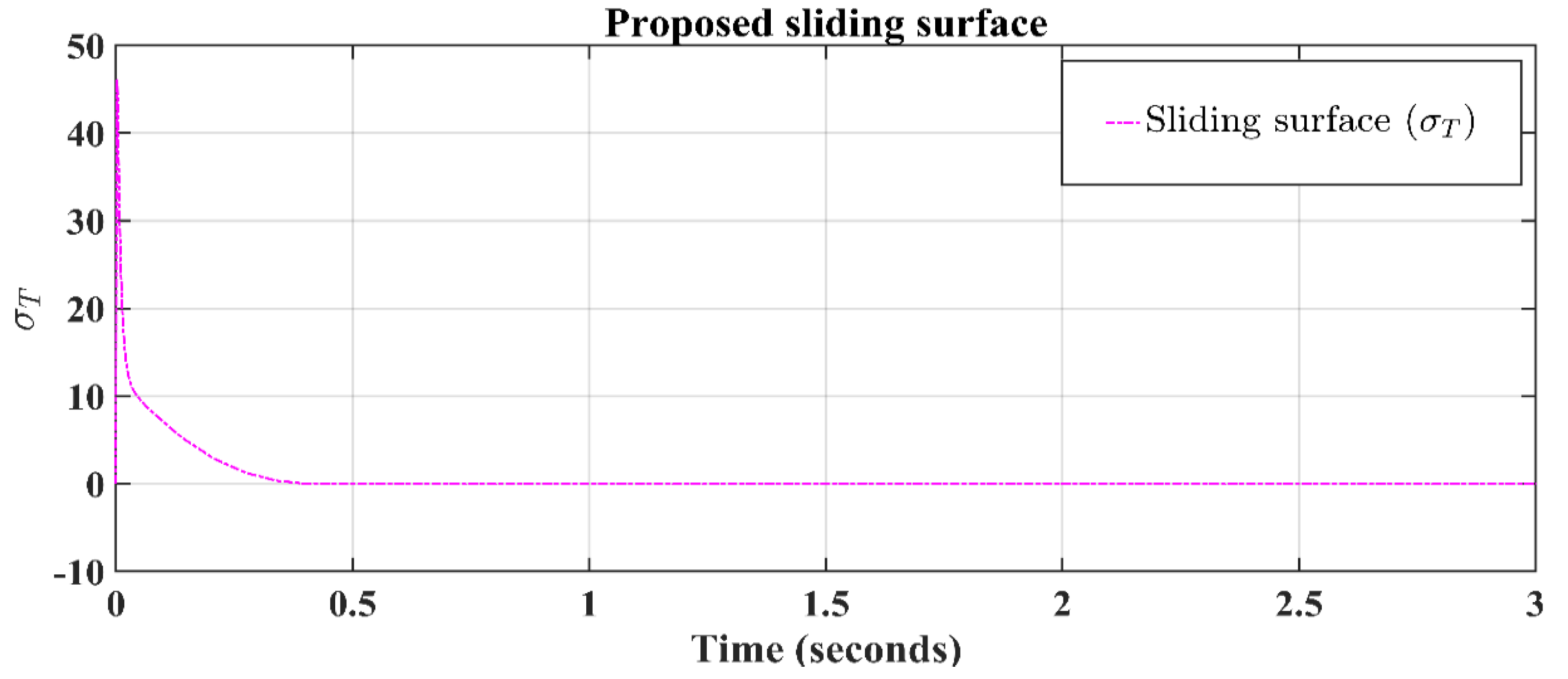
Figure 5 represents the total backstepping ISMC surface response for designing HGO-based proposed control algorithms. It can be observed that the system trajectories reach the sliding manifold in 0.5 s i.e., σ T = 0     t 0.5 
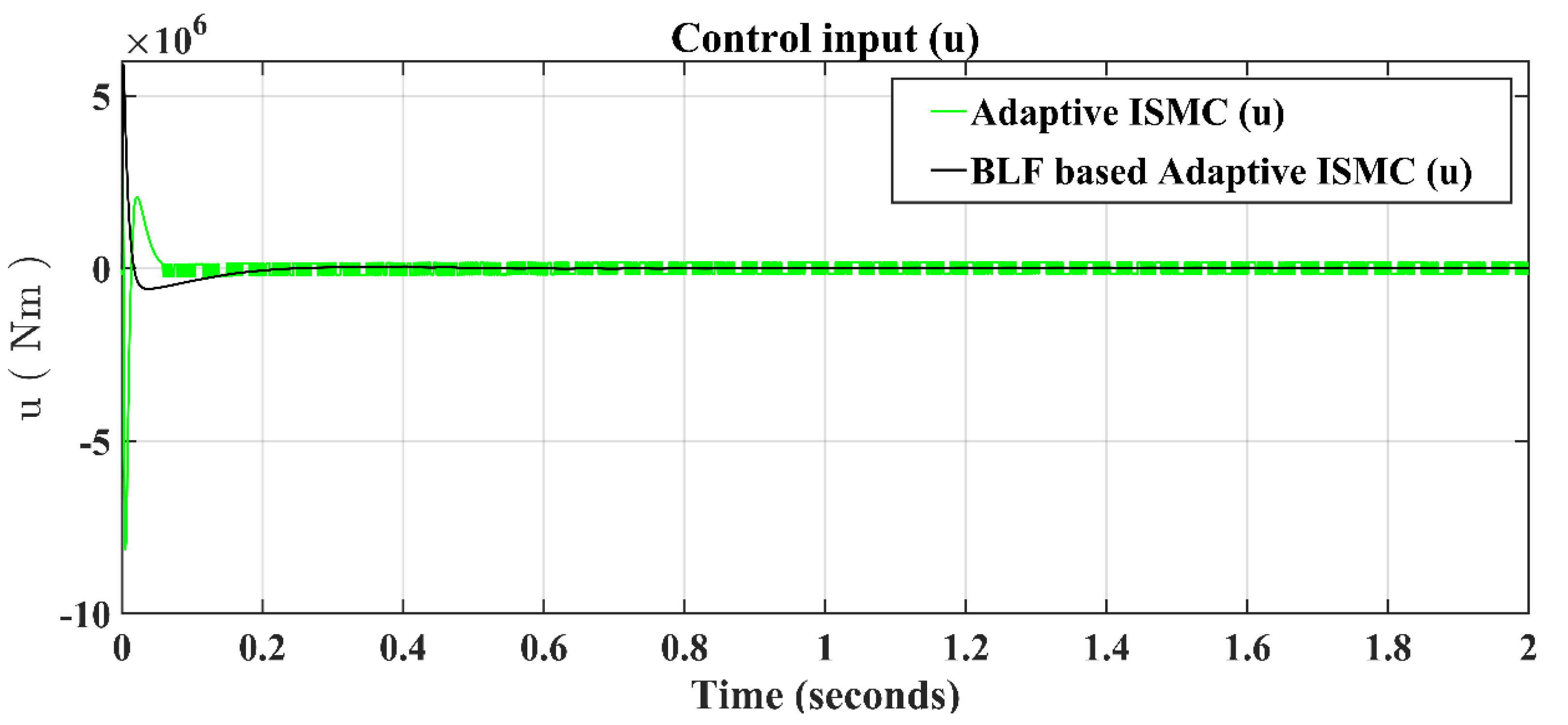
. The BLF-based adaptive backstepping ISMC input represents significantly less chattering than the adaptive backstepping ISMC input, as can be seen clearly in 
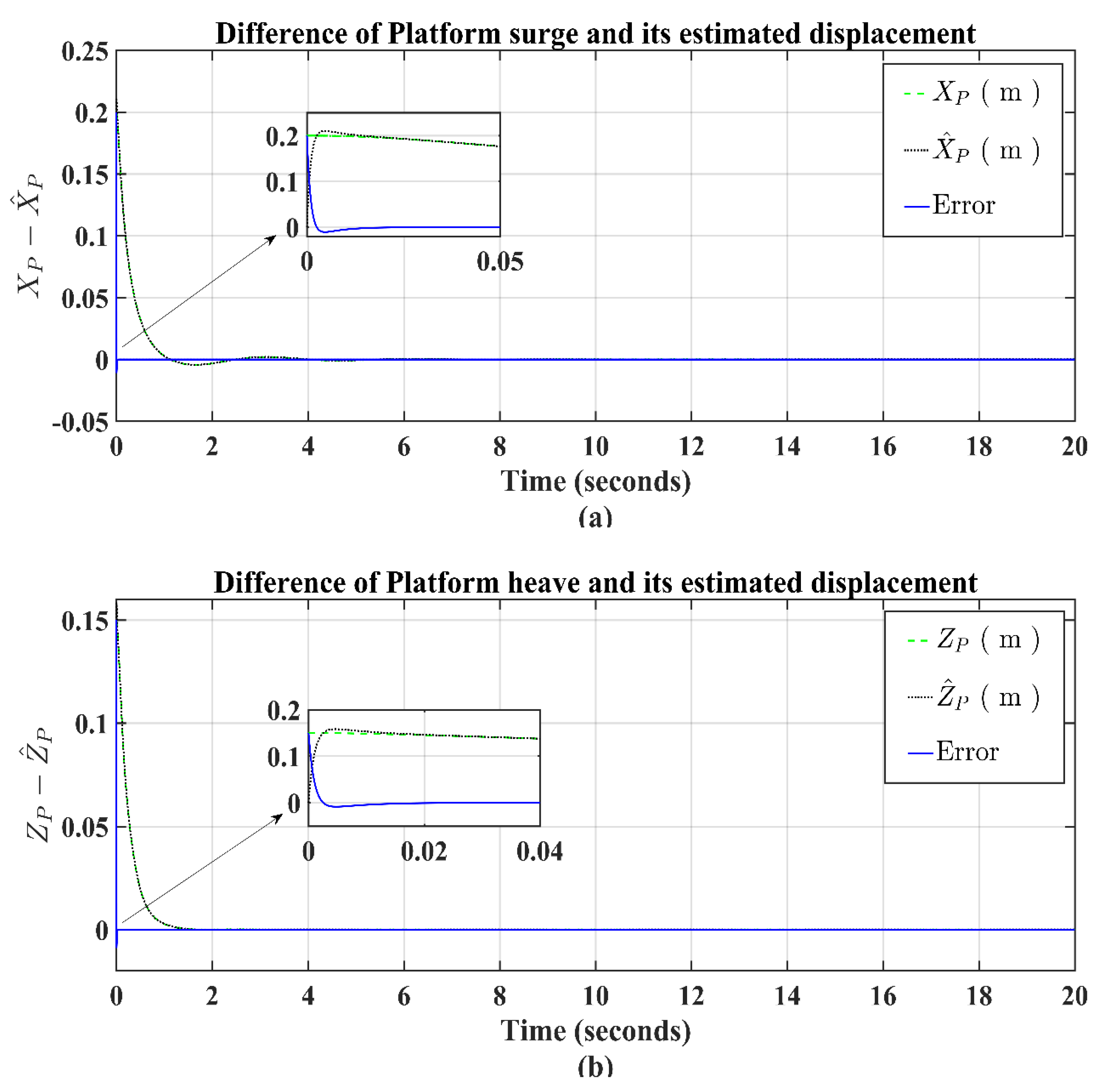
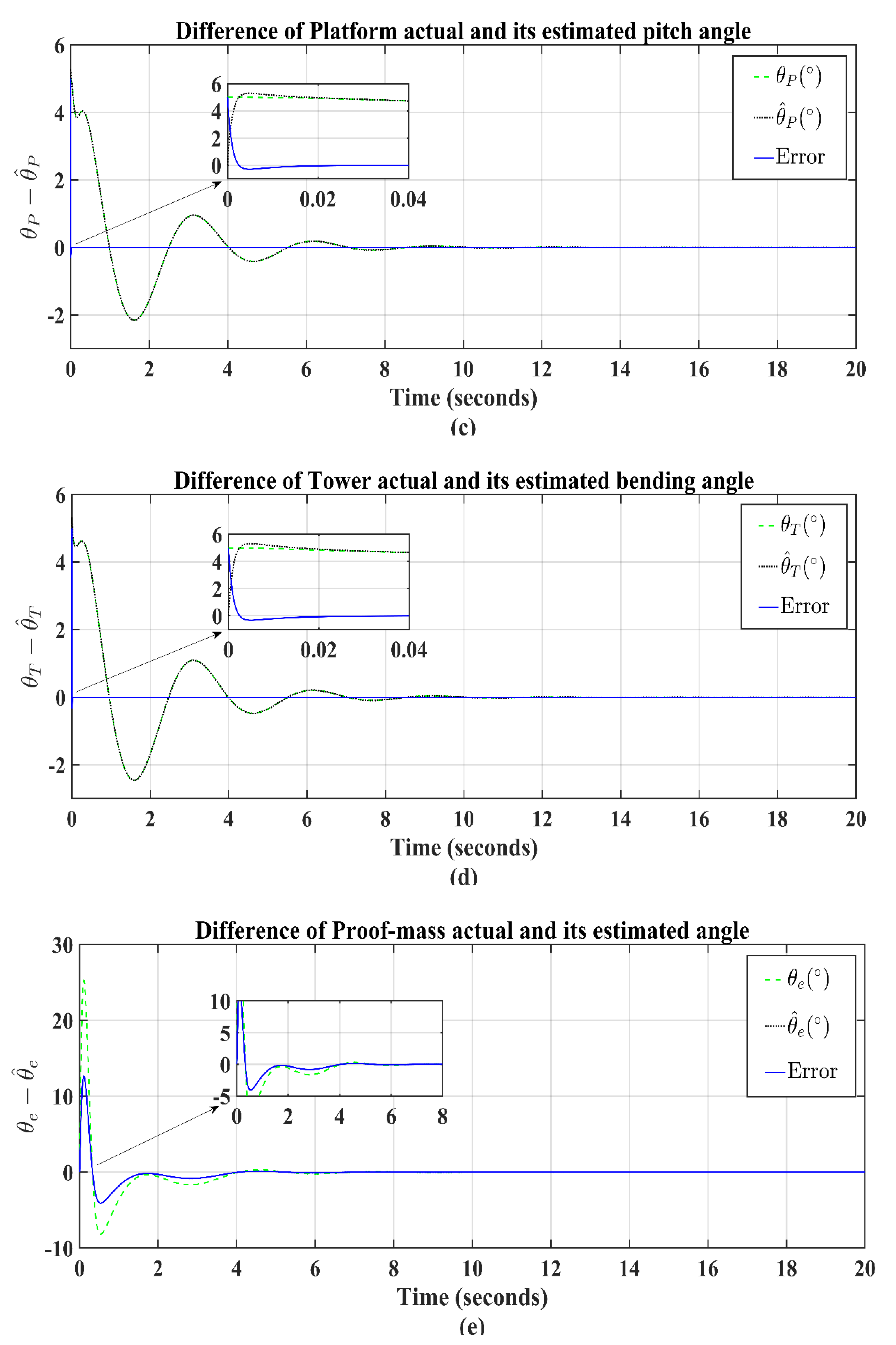
Figure 6. Using the HGO for the BLF−based adaptive backstepping ISMC, the original states and their estimated states with the respective error of the suggested model are shown in Figure 7, where the numerical difference between the original and their estimated states are very minor, as shown in 
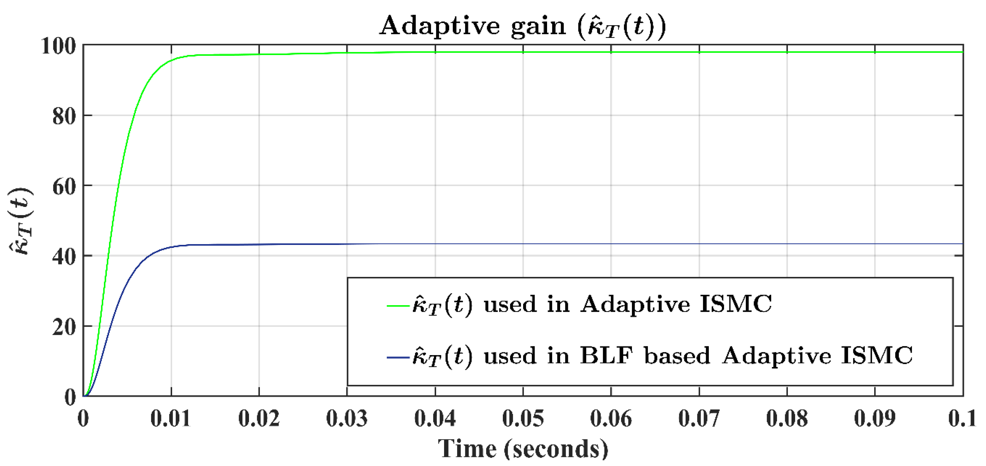
Table 2. This model works for all of the hypotheses provided in the modeling section. The response of the adaptive gains used in the adaptive backstepping ISMC and BLF-based adaptive backstepping ISMC algorithms are shown in Figure 8, where the adaptive gain used in the adaptive backstepping ISMC settles at approximately 97 and the adaptive gain used in the BLF-based adaptive backstepping ISMC settles at approximately 43.

6. Conclusions

The TORA as an AMD control strategy for the stabilization of the barge-type 5DOF OFWT model is challenging and interesting. In this article, a novel control framework has been devised that consists of a high-gain observer-based adaptive integral sliding mode control with backstepping and barrier Lyapunov function. This control algorithm successfully solved the issue of the unavailability of the system states by providing all the proposed OFWT model estimated states. The numerical simulations and their numeric error table reveal that the proposed output constraint BLF-based adaptive backstepping ISMC can effectively handle vibrations as compared with the adaptive backstepping ISMC. In both control laws, the proposed model states go to their equilibrium position within 10 s, but the difference is that the BLF-based adaptive backstepping ISMC guarantees to satisfy the constraint on the states. Moreover, the proposed output constraint BLF-based adaptive backstepping ISMC shows less chattering than the adaptive backstepping ISMC. The results confirm the validity and efficiency of the suggested control approaches. The floating wind turbine structures are thus far at an early stage of development and various platforms are in a proof-of-concept study using a scale model incorporating a barge, spar, and tension leg platform. Therefore, more research on this topic is still required. Future work will consider model gearboxes and actuation components that produce the control input torque, like hydraulic or electric motors. Similarly, comparing the simulation results of this proposed model by using other simulation tools (FAST/SIMPACK) as well as experimental results can be conducted.

Author Contributions

Conceptualization, S.A.A.S. and B.G.; methodology, S.A.A.S. and B.G.; formal analysis, B.G., I.A. and H.U.; writing—original draft, S.A.A.S.; writing—review and editing, H.U., N.A. and A.S.; validation, S.A.A.S., B.G. and I.A.; visualization, N.A. and A.S.; supervision, B.G.; funding acquisition, B.G. All authors have read and agreed to the published version of the manuscript.

Funding

This research received no external funding.

Institutional Review Board Statement

Not applicable.

Informed Consent Statement

Not applicable.

Data Availability Statement

Not applicable.

Conflicts of Interest

The authors declare no conflict of interest.

Appendix A. Matrices

Following are the matrices derived in the stability analysis of high-gain observer for the suggested barge-type OFWT model.
A = 0 1 0 0 0 0 0 0 0 0 0 0 0 0 0 0 0 0 0 0 0 0 0 1 0 0 0 0 0 0 0 0 0 0 0 0 0 0 0 0 0 0 0 0 0 1 0 0 0 0 0 0 0 0 0 0 0 0 0 0 0 0 0 0 0 0 0 1 0 0 0 0 0 0 0 0 0 0 0 0 0 0 0 0 0 0 0 0 0 1 0 0 0 0 0 0 0 0 0 0
B = 0 1 0 0 0 0 0 0 0 0 0 0 0 1 0 0 0 0 0 0 0 0 0 0 0 0 0 0 0 0 0 0 0 0 0 0 0 1 0 0 0 0 0 0 0 0 0 0 0 1 T
C = 1 0 0 0 0 0 0 0 0 0 0 0 1 0 0 0 0 0 0 0 0 0 0 0 1 0 0 0 0 0 0 0 0 0 0 0 1 0 0 0 0 0 0 0 0 0 0 0 1 0
H = γ 1 γ 2 0 0 0 0 0 0 0 0 0 0 γ 3 γ 4 0 0 0 0 0 0 0 0 0 0 γ 5 γ 6 0 0 0 0 0 0 0 0 0 0 γ 7 γ 8 0 0 0 0 0 0 0 0 0 0 γ 9 γ 10 T
A 0 = γ 1 1 0 0 0 0 0 0 0 0 γ 2 0 0 0 0 0 0 0 0 0 0 0 γ 3 1 0 0 0 0 0 0 0 0 γ 4 0 0 0 0 0 0 0 0 0 0 0 γ 5 1 0 0 0 0 0 0 0 0 γ 6 0 0 0 0 0 0 0 0 0 0 0 γ 7 1 0 0 0 0 0 0 0 0 γ 8 0 0 0 0 0 0 0 0 0 0 0 γ 9 1 0 0 0 0 0 0 0 0 γ 10 0
B 0 = 0 1 0 0 0 0 0 0 0 0 0 0 0 1 0 0 0 0 0 0 0 0 0 0 0 1 0 0 0 0 0 0 0 0 0 0 0 1 0 0 0 0 0 0 0 0 0 0 0 1 T
D b = b 0 0 0 0 0 0 0 0 0 0 1 0 0 0 0 0 0 0 0 0 0 b 0 0 0 0 0 0 0 0 0 0 1 0 0 0 0 0 0 0 0 0 0 b 0 0 0 0 0 0 0 0 0 0 1 0 0 0 0 0 0 0 0 0 0 b 0 0 0 0 0 0 0 0 0 0 1 0 0 0 0 0 0 0 0 0 0 b 0 0 0 0 0 0 0 0 0 0 1
ζ = a 1 1 1 0 0 0 0 0 0 0 0 a 2 1 0 0 0 0 0 0 0 0 0 0 0 a 1 2 1 0 0 0 0 0 0 0 0 a 2 2 0 0 0 0 0 0 0 0 0 0 0 a 1 3 1 0 0 0 0 0 0 0 0 a 2 3 0 0 0 0 0 0 0 0 0 0 0 a 1 4 1 0 0 0 0 0 0 0 0 a 2 4 0 0 0 0 0 0 0 0 0 0 0 a 1 5 1 0 0 0 0 0 0 0 0 a 2 5 0

References

  1. Wang, S.; Wang, S. Impacts of wind energy on environment: A review. Renew. Sustain. Energy Rev. 2015, 49, 437–443. [Google Scholar] [CrossRef]
  2. Liu, Y.; Xiao, Q.; Incecik, A.; Wan, D.C. Investigation of the effects of platform motion on the aerodynamics of a floating offshore wind turbine. J. Hydrodyn. 2016, 28, 95–101. [Google Scholar] [CrossRef] [Green Version]
  3. Pérez-Collazo, C.; Greaves, D.; Iglesias, G. A review of combined wave and offshore wind energy. Renew Sustain. Energy Rev. 2015, 42, 141–153. [Google Scholar] [CrossRef] [Green Version]
  4. Lackner, M.A.; Rotea, M.A. Structural control of floating wind turbines. Mechatronics 2011, 21, 704–719. [Google Scholar] [CrossRef]
  5. Stewart, G.M. Load Reduction of Floating Wind Turbines Using Tuned Mass Dampers. 2012. Available online: https://scholarworks.umass.edu/theses/781/ (accessed on 20 February 2023).
  6. Lalonde, E.R.; Dai, K.; Bitsuamlak, G.; Lu, W.; Zhao, Z. Comparison of semi-active and passive tuned mass damper systems for vibration control of a wind turbine. Wind Struct. 2020, 30, 663–678. [Google Scholar]
  7. M’zoughi, F.; Garrido, I.; Garrido, A.J.; De La Sen, M. Fuzzy Airflow-Based Active Structural Control of Integrated Oscillating Water Columns for the Enhancement of Floating Offshore Wind Turbine Stabilization. Int. J. Energy Res. 2023, 2023, 4938451. [Google Scholar] [CrossRef]
  8. Ahmad, I.; M’zoughi, F.; Aboutalebi, P.; Garrido, I.; Garrido, A.J. Fuzzy logic control of an artificial neural network-based floating offshore wind turbine model integrated with four oscillating water columns. Ocean Eng. 2023, 269, 113578. [Google Scholar] [CrossRef]
  9. He, E.M.; Hu, Y.Q.; Zhang, Y. Optimization design of tuned mass damper for vibration suppression of a barge-type offshore floating wind turbine. Proc. Inst. Mech. Eng. Part M J. Eng. Marit. Environ. 2017, 231, 302–315. [Google Scholar] [CrossRef]
  10. Hu, Y.; Wang, J.; Chen, M.Z.; Li, Z.; Sun, Y. Load mitigation for a barge-type floating offshore wind turbine via inerter-based passive structural control. Eng. Struct. 2018, 177, 198–209. [Google Scholar] [CrossRef]
  11. Gavgani, S.A.M.; Jalali, H.H.; Farzam, M.F. Semi-active control of jacket platforms under wave loads considering fluid-structure interaction. Appl. Ocean Res. 2021, 117, 102939. [Google Scholar] [CrossRef]
  12. Park, S.; Lackner, M.A.; Pourazarm, P.; Rodríguez, T.A.; Cross-Whiter, J. An investigation on the impacts of passive and semiactive structural control on a fixed bottom and a floating offshore wind turbine. Wind Energy 2019, 22, 1451–1471. [Google Scholar] [CrossRef]
  13. Shah, S.A.A.; Gao, B.; Ahmed, N.; Liu, C. Advanced robust control techniques for the stabilization of translational oscillator with rotational actuator based barge-type OFWT. Proc. Inst. Mech. Eng. Part M J. Eng. Marit. Environ. 2021, 235, 327–343. [Google Scholar] [CrossRef]
  14. Shah, S.A.A.; Gao, B.; Bhatia, A.K.; Liu, C.; Rauf, A. Anti-vibration control design for TORA based barge-type offshore floating wind turbine using extended order high gain observer. Eng. Comput. 2022, 39, 2705–2732. [Google Scholar] [CrossRef]
  15. Frank, M.S.; Leylaz, G.; Sun, J.Q. Data-driven robust tracking control of underactuated mechanical systems using identified flat output and active disturbance rejection control. Int. J. Control 2021, 95, 3101–3117. [Google Scholar] [CrossRef]
  16. Ahmed, N.; Raza, A.; Shah, S.A.A.; Khan, R. Robust composite-disturbance observer based flight control of quadrotor attitude. J. Intell. Robot. Syst. 2021, 103, 11. [Google Scholar] [CrossRef]
  17. He, B.; Wang, S.; Liu, Y. Underactuated robotics: A review. Int. J. Adv. Rob. Syst. 2019, 16, 1–29. [Google Scholar] [CrossRef] [Green Version]
  18. Ahmed, N.; Ali Shah, S.A. Adaptive output-feedback robust active disturbance rejection control for uncertain quadrotor with unknown disturbances. Eng. Comput. 2022, 39, 1473–1491. [Google Scholar] [CrossRef]
  19. Liu, C.; Yu, C.; Gao, B.; Ali Shah, S.A.; Tapus, A. Towards a balancing safety against performance approach in human–robot co-manipulation for door-closing emergencies. Complex Intell. Syst. 2022, 8, 2859–2871. [Google Scholar] [CrossRef]
  20. Yu, Z.; Guo, Y.-B.; Zhang, X.-H. Stability control of TORA with environmental disturbance. In Proceedings of the 27th IEEE Chinese Control and Decision Conference (2015 CCDC), Qingdao, China, 23–25 May 2015; pp. 6107–6110. [Google Scholar] [CrossRef]
  21. Liu, C.; Gao, B.; Zhao, J.; Shah, S.A.A. Orbitally stabilizing control for the underactuated translational oscillator with rotational actuator system: Design and experimentation. Proc. Inst. Mech. Eng. Part I J. Syst. Control. Eng. 2019, 233, 491–500. [Google Scholar] [CrossRef]
  22. Shah, S.A.A.; Gao, B.; Ahmed, N.; Liu, C.; Rauf, A. Disturbance observer-based sliding mode control of TORA system for floating wind turbines. In Proceedings of the IEEE 9th Annual International Conference on CYBER Technology in Automation, Control, and Intelligent Systems (CYBER), Suzhou, China, 29 July–2 August 2019; pp. 418–423. [Google Scholar] [CrossRef]
  23. Saleh, B.; Yousef, A.M.; Ebeed, M.; Abo-Elyousr, F.K.; Elnozahy, A.; Mohamed, M.; Abdelwahab, S.A.M. Design of PID controller with grid connected hybrid renewable energy system using optimization algorithms. J. Electr. Eng. Technol. 2021, 16, 3219–3233. [Google Scholar] [CrossRef]
  24. Saleh, B.; Yousef, A.M.; Abo-Elyousr, F.K.; Mohamed, M.; Abdelwahab, S.A.M.; Elnozahy, A. Performance analysis of maximum power point tracking for two techniques with direct control of photovoltaic grid-connected systems. Energy Sources Part A Recovery Util. Environ. Eff. 2022, 44, 413–434. [Google Scholar] [CrossRef]
  25. Rauf, A.; Zafran, M.; Khan, M.S.A.; Khan, A.; Shah, S.A.A. Non-singular terminal sliding mode control of converter-fed DC motor system with mismatched disturbance compensation. Int. J. Model. Identif. Control 2021, 39, 285–292. [Google Scholar] [CrossRef]
  26. Ahmed, N.; Bhatia, A.K.; Shah, S.A.A. Robust active disturbance attenuation control of an uncertain quadrotor. Int. J. Intell. Unmanned Syst. 2021, 10, 346–362. [Google Scholar] [CrossRef]
  27. Zhang, Y.; Zhao, X.; Wei, X. Robust structural control of an underactuated floating wind turbine. Wind Energy. 2020, 23, 2166–2185. [Google Scholar] [CrossRef]
  28. Shah, S.A.A.; Malik, F.M.; Raza, A.; Khan, R.; Ahmed, N. Sampled data gyroscope stabilization of two degree of freedom platform. In Proceedings of the 13th IEEE International Bhurban Conference on Applied Sciences and Technology (IBCAST), Islamabad, Pakistan, 12–16 January 2016; pp. 251–255. [Google Scholar]
  29. Yoo, D.S. Design of integral sliding mode control for underactuated mechanical systems. J. Korean Inst. Intell. Syst. 2013, 23, 208–213. [Google Scholar]
  30. Al-Dujaili, A.Q.; Humaidi, A.J.; Pereira, D.A.; Ibraheem, I.K. Adaptive backstepping control design for ball and beam system. Int. Rev. Appl. Sci. Eng. 2021, 2, 211–221. [Google Scholar] [CrossRef]
  31. Mu, D.; Wang, G.; Fan, Y.; Qiu, B.; Sun, X. Adaptive trajectory tracking control for underactuated unmanned surface vehicle subject to unknown dynamics and time-varing disturbances. Appl. Sci. 2018, 8, 547. [Google Scholar] [CrossRef] [Green Version]
  32. Bhatia, A.K.; Jiang, J.; Kumar, A.; Shah, S.A.A.; Rohra, A.; Zhen, Z. Adaptive preview control with deck motion compensation for autonomous carrier landing of an aircraft. Int. J. Adapt. Control Signal Process. 2021, 35, 769–785. [Google Scholar] [CrossRef]
  33. Raza, A.; Malik, F.M.; Mazhar, N.; Khan, R. Two-time-scale robust output feedback control for aircraft longitudinal dynamics via sliding mode control and high-gain observer. Alex. Eng. J. 2021, 61, 4573–4583. [Google Scholar] [CrossRef]
  34. Baala, Y.; Bri, S. DFIG-Based Wind Turbine Control Using High-Gain Observer. In Proceedings of the 1st International IEEE Conference on Innovative Research in Applied Science, Engineering and Technology (IRASET), Meknes, Morocco, 16–19 April 2020; pp. 1–5. [Google Scholar] [CrossRef]
  35. Khalil, H.K. Nonlinear Systems, 3rd ed.; Patience Hall: Hoboken, NJ, USA, 2002; p. 115. [Google Scholar]
Figure 1. Barge-type TORA-based 5DOF OFWT model.
Jmse 11 00492 g001
Figure 2. Schematic diagram of the adaptive robust control scheme for OFWT system.
Jmse 11 00492 g002
Figure 3. The response of barge−type 5DOF TORA−based OFWT without applying control laws, (a) X P , (b) Z P , (c) θ P , (d) θ T , and (e) θ e , where brown results do not apply the proof-mass actuator in the OFWT model and green results do apply the proof-mass actuator in the OFWT model.
Jmse 11 00492 g003aJmse 11 00492 g003b
Figure 4. The response of barge−type 5DOF TORA−based OFWT when using adaptive backstepping ISMC and BLF-based adaptive backstepping ISMC, (a) X P , (b) Z P , (c) θ P , (d) θ T , and (e) θ e , where brown results represent adaptive backstepping ISMC efficiency and green results represent BLF-based adaptive backstepping ISMC efficiency.
Jmse 11 00492 g004aJmse 11 00492 g004b
Figure 5. The response of the total backstepping ISMC surface ( σ T ) for developing proposed control algorithms.
Jmse 11 00492 g005
Figure 6. The response of the proposed control inputs, where green represents adaptive backstepping ISMC efficiency and black represents BLF−based adaptive backstepping ISMC efficiency.
Jmse 11 00492 g006
Figure 7. Simulation results of the controlled barge−type 5DOF TORA−based OFWT for the actual states (green) and their estimated states (black), and corresponding error (blue color): (a) Difference between platform surge and its estimated displacement, (b) Difference between platform heave and its estimated displacement, (c) Difference between platform’s actual and its estimated pitch angle, (d) Difference between tower’s actual and its estimated bending angle, (e) Difference between proof mass actual and its estimated angle.
Jmse 11 00492 g007aJmse 11 00492 g007b
Figure 8. The response of the adaptive gain used in adaptive backstepping ISMC (green) and BLF-based adaptive backstepping ISMC (blue).
Jmse 11 00492 g008
Table 1. Proposed control tuning parameters.
ParametersValueParametersValue
α 1 3 λ 5 10
α 2 3 ν 0 1
α 3 3 ν 1 1
α 4 2 ω 0 5
α 5 1 ω 1 5
λ 1 1 η 10
λ 2 1 Ω T 10
λ 3 1 a 1 11
λ 4 1 a 2 11
Table 2. Error analysis of the controlled states (CS) and estimated states (ES).
Signal under ObservationError X P Z P θ P θ T θ e
CS using adaptive ISMCTransient state0.02910.02101.16481.28931.2992
Steady state0.00010.00010.00610.00700.0116
RMSE0.01580.01140.82080.90840.9155
CS using BLF-based adaptive ISMCTransient state0.02890.02111.17781.31083.4688
Steady state0.00010.00010.00630.00700.0102
RMSE0.01570.01140.82990.92362.4443
ES using HGORMSE0.00510.00380.12790.12791.2221
Disclaimer/Publisher’s Note: The statements, opinions and data contained in all publications are solely those of the individual author(s) and contributor(s) and not of MDPI and/or the editor(s). MDPI and/or the editor(s) disclaim responsibility for any injury to people or property resulting from any ideas, methods, instructions or products referred to in the content.

