Article

Simulating the Impacts of an Applied Dynamic Adaptive Pathways Plan Using an Agent-Based Model: A Tauranga City, New Zealand, Case Study

1
National Institute of Water and Atmospheric Research, Hamilton 3216, New Zealand
2
Climate Change Research Institute, Victoria University Wellington, Wellington 6012, New Zealand
3
School of Environment, The University of Auckland, Auckland 1142, New Zealand
*
Author to whom correspondence should be addressed.
J. Mar. Sci. Eng. 2023, 11(2), 343; https://doi.org/10.3390/jmse11020343
Submission received: 29 November 2022 / Revised: 19 January 2023 / Accepted: 30 January 2023 / Published: 4 February 2023
(This article belongs to the Topic Coastal Development, Conservation and Sustainability)

Abstract

:
Climate change and relative sea-level rise (RSLR) will increasingly expose coastal cities to coastal flooding, erosion, pluvial and fluvial flooding, episodic storm-tide flooding and eventually, permanent inundation. Tools are needed to support adaptive management approaches that allow society to adapt incrementally by making decisions now without creating path dependency and compromising decision-making options in the future. We developed an agent-based model that integrates climate-related physical hazard drivers and socio-economic drivers. We used it to explore how adaptive actions might be sequentially triggered within a low-elevation coastal city in New Zealand, in response to various climate change and socio-economic scenarios. We found that different adaptive actions are triggered at about the same RSLR level regardless of shared socio-economic pathway/representative concentration pathway scenario. The timing of actions within each pathway is dictated mainly by the rate of RSLR and the timing and severity of storm events. For the representative study site, the model suggests that the limits for soft and hard protection will occur around 30 cm RSLR, fully-pumped water systems are viable to around 35 cm RSLR and infrastructure upgrades and policy mechanisms are feasible until between 40 cm and 75 cm RSLR. After 75 cm RSLR, active retreat is the only remaining adaptation pathway.

1. Introduction

Climate change and relative sea-level rise (RSLR) create challenges for coastal cities. They will be increasingly exposed to coastal flooding, erosion, pluvial and fluvial flooding, episodic storm-tide flooding and even permanent inundation [1,2]. Globally, many cities are exposed to these hazards [2,3], and the risk continues to rise with increasing global greenhouse gas (GHG) emissions in addition to that already in the system from past GHG emissions; there is a lag time and we have not yet seen all the impacts of past emissions. Analysis of the interactions of these hazards with the built environment is becoming increasingly important to planners and decision-makers. Firstly, because they reflect current realities at the coast where hazards frequently occur simultaneously (e.g., storms can lead to a combination of storm surge-driven inundation, pluvial and fluvial flooding, groundwater impacts and saline intrusion hazards [1,4]). Secondly, because such events can have high social and economic costs (i.e., displacement of people and communities, financial costs of business disruption and impacts on insurance premiums and availability [5,6,7]). Thirdly, because future impacts of climate change and sea-level rise (SLR) will exacerbate the magnitude, frequency and severity of coastal hazards [2,8,9].
Complicating the ability to adapt to future change is the challenge of deep uncertainty [10] in future climate-driven change to sea-level rise (SLR) and coastal hazards [11]. There are a variety of assessment methodologies available for environmental change. Traditionally used methods such as cost-benefit analysis have long been popular [12]. Multi-criteria analysis is commonly used when impacts cannot be converted to a common metric [13]. Real options analyses, on the other hand, take into account time flexibility and irreversible costs [14], but are still usually based on an underlying assumption that values can be quantified and optimised. A modified application of real options analysis has been developed that avoids these limitations in situations of deep uncertainty associated with changing climate that stress tests options rather than optimises them [15]. These conventional methods can also under-estimate the uncertainties around the impact of wellbeing values, which are magnified by the changing climate risks. Economic tools are designed to optimise wellbeing subject to a quantifiable level of risk, but true uncertainty calls for different practical tools that instead focus on robustness and can develop options that perform across a range of plausible futures [16,17].
One way to address uncertainty is to test outcomes against plausible scenarios—hence the Intergovernmental Panel on Climate Change (IPCC) developed several GHG emission representative concentration pathway (RCP) scenarios [18,19], each having a different rate of SLR. These scenarios are periodically updated as better information becomes available and simulation methods improve [18,19]. The uncertainty in SLR increases with time—the range between the median SLR projections for the lowest emissions scenario in AR5 (RCP2.6) and highest emissions scenario (RCP8.5) is 0.02 m by 2030 and 0.33 m by 2100 (relative to 1986–2005 baseline mean sea-level) [19]; the range difference between the low-end of RCP2.6 and the high-end of RCP8.5 is 70 cm by 2100 [19]. There is also deep uncertainty around the way in which society can adapt under different emission scenarios, represented by the IPCC shared socio-economic pathways (SSP) [20]. While the most recent IPCC AR6 reports [18] have linked RCPs and SSPs, these linkages are subject to future revisions. The uncertainty around both physical scenarios and socio-economic responses to change still remains. Regardless of future global emissions, the world will experience more than one metre of SLR, of uncertain timing, due to the temporal lag effects of historic emissions [21]. Nevertheless, there is certainty of sea levels out to mid-century [11,22]. Hence, multiple scenarios or sea-level rise increments can be used to stress-test potential policy options for their robustness under a range of conditions [23].
This raises the question of how to respond in the face of such deep uncertainty in the future. Many adaptation actions, policies and decisions have a limited design-life under rising seas and may fail under future socio-economic or climatic conditions [24]. In addition, some adaptation actions taken in the present have the potential to increase the exposure of human and natural systems to SLR which will continue for centuries—therefore, maladapted [18]. This occurs at the coast where increased development in exposed locations creates lock-in of a fixed development path, such as through protection actions that create a false sense of security and will reach hard limits as the sea rises and coastal storms become more intense [25]. Switching from the dominant predict-and-act coastal management strategies to approaches that allow society to anticipate a range of actions and take initial actions that leave future options open depending on how the future progresses, can help reduce the effect of lock-in of people and assets. Such dynamic adaptive approaches enable flexible decisions to be made in the present while maintaining the ability to change strategy in the future [26]. Such approaches can avoid decisions that become insufficient as the sea levels progressively rise and can also enable transformational adaptations, such as planned relocation and coastal realignment, to be staged as required [27,28,29,30,31]. For example, increasing seawall height incrementally will reach physical and affordability limits because of ongoing sea-level rise and increasing intensity of coastal storms. Meanwhile, increasing development behind seawalls creates greater residual risk as limits of protection are exceeded, exposing more assets and people requiring a shift to active retreat (transformational adaptation) [12]. Decision tools and models can assist decision-making that can help avoid maladaptation and inform more effective adaptation options and account for social, political, economic, cultural and environmental factors that drive spatial and temporal decisions in coastal areas while addressing deep uncertainty surrounding them [32,33].
There are several decision-making processes available that facilitate pre-emptive adaptation decisions and which address uncertainty and changing risk in situations where the stressor is ongoing, such as SLR [8,10,23,24]. Dynamic Adaptive Pathways Planning (DAPP) is one such method and has emerged as a ‘fit-for-purpose’ method for climate change adaptation planning to address widening future uncertainty where the risk is changing over long planning timeframes [8].
A DAPP for example can be developed and visualised as a series of alternative actions that can be implemented over time, forming a number of pathways; a new action can be implemented when conditions change, and the current or original action no longer achieves its objectives [24]. At that point, an alternative action and pathway can be adopted before the adaptation threshold (failure) is reached. Box 1 defines the terminology and Box 2 provides a list of abbreviations used in this paper.
Box 1. DAPP terminology.
Indicator: Also known as a ‘signpost’ [8,34]. “Specify information that should be tracked in order to determine whether the plan is meeting the conditions for its success” ([26], p. 487).
Signal: Also known as an ‘early warning signal’. Value of an indicator variable that suggests that the trigger may be approaching [24].
Trigger: “Critical values of indicator variables beyond which additional actions should be implemented” ([26], p. 487).
Action: An adaptation action selected following a Trigger and applied after the lead time [26].
Lead time: The time it takes to implement an action after the Trigger is reached; actions usually cannot be implemented immediately [26].
Adaptation threshold: Also known as an ‘adaptation tipping point’ [8,34]. “The point at which a particular action is no longer adequate or meeting the plan’s objectives” ([26], p. 486).
Box 2. Abbreviations.
ABM: agent-based modelling/agent-based model
DAPP: dynamic adaptive pathways planning/dynamic adaptive pathways plan
GHG: greenhouse gas
MHCABM: Multi-Hazard Coastal Agent-Based Model
RCP: Representative Concentration Pathway
RSLR: relative sea level-rise
SLR: sea level-rise
SSP: Shared Socio-economic Pathway
VLM: vertical land movement
A key component of DAPP is the monitoring of change using indicators that can be environmental, social, political, economic or cultural. When an indicator signals a change in conditions the decision maker is alerted that a trigger is approaching, and a review can be undertaken to establish which next actions and pathway can reach the objectives. This enables the decision for timely adaptive actions (Figure 1). Signals provide early warning of the emergence of the trigger and the trigger initiates a process to change adaptive action before a harmful adaptation threshold is reached (e.g., Figure 2) [35,36,37,38]. Such a system of signals and triggers can be included within a DAPP framework and forms the basis of the monitoring of the changes [25].
Some of the key challenges in designing a DAPP include the identification of appropriate indicators and associated adaptation thresholds, setting the value for each trigger (e.g., the amount of SLR that triggers an action to be taken), identifying appropriate actions that could meet objectives once the trigger is activated, and stress testing the implications of alternative sequences of adaptive actions (pathways) under a range of different climatic and socio-economic scenarios.
In this paper we describe an exploratory modelling approach where a DAPP is developed, and signals and triggers are coded into an agent-based model (ABM) as an integrated submodel. DAPP has previously been used in conjunction with a variety of modelling and decision support approaches (e.g., [10,39,40]). Haasnoot et al. [17] suggested that integrating DAPP into an ABM could be a method of developing and exploring pathways.
Agent-based modelling (ABM) simulates the interactions between autonomous agents, and the mutual interactions and feedbacks between agents and their environment. An ‘agent’ is any autonomous entity that makes decisions for itself. ABMs can be more revealing of the interactions of individual values and agents than comparative modelling techniques such as system dynamics models or Bayesian networks [41,42]. ABM is a particularly useful approach for simulating the interactions between human and environment components of coastal systems (e.g., [43,44,45]).
Much previous work in the uncertainty modelling space has focused on technical data rather than the role of human agency. In the DAPP processes used to date, human behavioural aspects have been included via MCDA assessments using participatory processes [46]. We suggest that by adding simple human behavioural rules via an ABM, we can gain new insights about the transition between, and timing of, different adaptive actions because individual and societal responses differ depending on what type of hazard event they are experiencing or have experienced. It is well established that hazards are not independent and often occur at the same time; for example, river flooding and storm tides occurring simultaneously [47]. However, simulation of the impacts of multiple interacting hazards is largely absent from the agent-based modelling literature, despite ABMs of flood risk being prevalent (e.g., [48,49]).
To demonstrate the value and future potential of combined ABM–DAPP models that integrate information from multiple disciplines, we follow a novel approach using a multi-hazard ABM with an integrated DAPP submodel called Multi-Hazard Coastal ABM (MHCABM) [50]. In combination, the models allow us to explore how adaptive actions might be sequentially triggered in response to hazard drivers in a coastal urban setting using a range of climate change and socio-economic scenarios, i.e., is there an adaptive pathway that emerges, or are there several pathways that meet the objectives, and what would they look like? Generating knowledge about how sequences of adaptive actions propagate and under what conditions would allow decision-makers the opportunity to proactively plan the implementation of adaptive actions. Equally, identifying potential opportunities to change the sequence of adaptive actions would provide greater flexibility for climate change adaptation at the coast. We developed the modelling framework in a New Zealand context where DAPP has been embedded in national coastal guidance [8,16] for application over the mandated “at least a 100 year” planning horizon, to assist in the implementation process of dynamic coastal pathways. In this paper we seek to achieve two objectives: (1) to identify common pathways of adaptive actions that would occur using this DAPP, and (2) to demonstrate the value and future potential of interdisciplinary ABM–DAPP models. Section 2 describes the methods used and Section 3 presents results from the exploratory modelling scenario analysis. Section 4 provides discussion and reflection on the process followed, with conclusions in Section 5.

2. Materials and Methods

To achieve the objectives, we developed a DAPP submodel, and integrated it in MHCABM.

2.1. Introduction—Model Components

MHCABM includes five interacting hazards—SLR, rainfall/runoff, inundation, erosion and rising groundwater—which are spatially overlain on a representation of Tauranga city (a New Zealand coastal city) and simulated over a 140-year period. MHCABM has three main component systems: geophysical, socio-economic and DAPP that are run in that order. The geophysical submodel is run first. It includes SSP/RCP, rainfall-runoff, storm events, and physical impacts of adaptation actions (e.g., seawall impacts on erosion); SSP runs at the same time as RCP in order for the geophysical system to respond to SSP drivers at the same timestep as the other systems. The socio-economic submodel is run second. It accounts for deprivation effects (based on the New Zealand Individual Index of Deprivation 2013 [51]), new building of homes and businesses, changes in desirability1 of property and movement of people. The DAPP submodel is run third. MHCABM controls the interaction of socio-economic and climate forcing (SSP and RCP) drivers and physical hazards, and their influence on the indicators through the sequential operation of five component submodels, as described in Appendix A.

2.2. Model Forcing

MHCABM is forced with SSPs linked to RCPs and RSLR projections (Figure 3) [20,52]. SSPs are shared socio-economic pathways that account for energy, land use, emissions and population changes and growth. SSPs are associated with different ways that society could react to changing climate; whether proactive as in the case of SSP1, reactive as in SSP3, or a combination of both as in SSP5. The SSP/RCP combinations have names and represent six plausible futures for New Zealand. For example, under scenario ‘Unspecific Pacific’ (SSP3/RCP8.5) we might expect fast SLR and less proactive adaptation, whereas under scenario ‘100% Smart’ (SSP1/RCP2.6) we might expect slower SLR and more proactive adaptation. The SSP/RCP scenarios use IPCC AR5 SLR projections, which have only subtle differences from the more recent AR6 scenarios that became available after model development.
The six SSP/RCP scenarios come from four RCPs (2.6, 4.5, 6.0 and 8.5) and three SSPs (1, 3 and 5). The use of multiple scenarios to stress-test adaptive actions in the face of deep uncertainty follows New Zealand guidance on coastal adaptation [23,54]. It is also recognition that uncertainty about the future impacts the modeler as well as the agents in the model.
The rules in MHCABM are independent of RCP but differ according to SSP. The key rule difference is in population growth. SSP1 and SSP5 projections show population peaking mid-21st century before a slow decline, whereas SSP3 projects population to continue to increase throughout the 21st century. This population growth is governed in the model by property desirability for new development, which gradually declines in SSP1 and SSP5 as population peaks and declines but does not decline in SSP3 as demand remains high. The ongoing high desirability of coastal property under SSP3 reflects agents in that scenario responding to SLR and coastal hazards reactively, whereas the declining desirability of coastal property in SSP1 and SSP5 reflects agents responding to SLR and coastal hazards, proactively.

2.3. Dynamic Adaptive Pathways Plan

A set of rules were developed using author expert judgement, based on our own experiences in coastal adaptation. These rules are described in Appendix A of this paper. The DAPP involves monitoring a set of eight indicators from five categories: financial, social, psychological, hazard and policy (Table 1). We established a set of adaptation thresholds for each indicator and a set of signals (warnings) and triggers (conditions for a change in adaptive action). The choice of indicator values for signals, triggers and adaptation thresholds (Table 2) was decided using author expert judgement, after seeking input from council infrastructure managers and reviewing local and international literature, in particular Lawrence et al. [25]. Each trigger was allocated a choice of plausible actions using author expert judgement. Each action chosen has a % likelihood of selection. The action ‘PR’ automatically instigates trigger ‘preparation for active retreat’, meaning that active retreat will begin after the 20-year lead time, with the current adaptation action remaining in place during the lead time. Active retreat has no signal or adaptation threshold, only a trigger; this trigger becomes active when any other trigger selects action ‘preparation for active retreat’ as its action. Preparation for active retreat combines the three preparatory stages set out in Lawrence et al. [55]—community engagement, planning and preparing, and enabling investment. Active retreat refers to the act of retreating from hazard-prone areas and is reliant on preparation for active retreat having occurred at the start of the DAPP development as one of the options—in many cases retreat will be inevitable and be triggered by indicators set out early and reviewed over the life of the pathways as the seas progress inland. The 20-year lead time for active retreat used in the model recognises the long time period required to initiate and undertake a successful managed retreat.
Actions and their lead time are further described in Table 2. Percentages represent pre-specified likelihood of action selection once the trigger is reached. Stressed houses are those that have been impacted by one or more hazard events but remain insurable. A patch is a spatial area unit representing one hectare.
There is a hardcoded lead time for each action; the lead time is the pre-emptive action required to allow a change in pathway to occur after a trigger (e.g., the time it takes to consent and construct a seawall). Thus, there is a series of rules within the DAPP model that controls pathway evolution in response to socio-economic, hazard and climate-change drivers.
The DAPP submodel checks whether any indicator value has met or exceeds the associated signal, trigger or adaptation threshold value and if it has, then the signal, trigger or adaptation threshold becomes ‘active’. Signals are monitored, but do not instigate a change in behaviour: they are purely a sign that a trigger may be approaching. When a trigger becomes active an action is selected, and each action has an associated lead time (Table 1). Once the lead time has elapsed, the selected action becomes the current action, and a new pathway is taken. If multiple triggers become active simultaneously a new action selection process is undertaken, in recognition of the impending threat of multiple adaptation thresholds being breached. The model was run in two ways: (1) with the pathway change function active, and (2) with the pathway change function inactive. This was to investigate the timing of signals, triggers and adaptation thresholds, both with and without the influence of pathway changes that may prevent or delay their occurrence.
The model includes several adaptive actions (Table 2), which are triggered by the interacting hazards according to a pre-specified series of rules (Table 1) coded into the DAPP. MHCABM includes stochasticity, as the occurrence of rainfall/runoff events are randomised, and the property values allocated to buildings are randomly assigned based on a distribution of values, meaning that the ability of individuals to take adaptive actions is different in each iteration of the model. For each SSP/RCP scenario the model is run using a 2500-iteration Monte Carlo approach, which results in many different pathways. The main stochastic variable is the timing and severity (condition) of storm impacts (storm tide and inundation); the storm tide is added to SLR and influences erosion and groundwater levels. From the 2500 iterations per SSP/RCP scenario, we extract the most common pathway that evolves in response to each SSP/RCP scenario when following our DAPP. Additionally, mean timings and distributions of each response variable (pathway, signal, trigger, adaptation threshold and action) are identified for each simulation group. This allows us to draw conclusions on how society may move along a DAPP pathway under different conditions.

2.4. Modeler Assumptions

We would expect RCP to have direct effects on the number of hazard impacts and their severity, because RCP is directly linked to SLR and the severity of heavy rainfall events. Fast SLR will mean that more houses and businesses are exposed to hazards and more quickly, whereas slower SLR will mean that fewer houses and businesses are exposed, and exposure will occur later. Therefore, if SLR was a key driver of adaptive actions, then we would expect ‘Unspecific Pacific’ (SSP3/RCP8.5) to have earlier triggering of adaptive actions than ‘100% Smart’ (SSP1/RCP2.6).
Individual agents in MHCABM respond to both chronic (RSLR) and acute (e.g., storm event) hazards by implementing adaptive actions; for example, constructing a seawall or raising floor levels of a building susceptible to hazards. In this manner, human behaviour is one of the drivers that influences overall system behaviour, which in turn impacts on signals, triggers and adaptation thresholds being reached. The decisions made in the DAPP are the equivalent of those made by regional government, which implements planning rules that are implemented by individual agents, and the decision-domain is residential dwellings and commercial properties.

2.5. Limitations

MHCABM is a simplified representation of a highly complex system. The way the rules play out in MHCABM is determined by the variables used to force the model, and the timing and severity of hazard events. Triggering of adaptive actions depends on the rules implemented in the MHCABM model, and model outcomes are sensitive to the rules. However, while the values for signals, triggers and adaptation thresholds and the lead time for actions are hardcoded, their timing and the condition drivers are not pre-determined. Instead, the timing of pre-determined actions is generated by the interaction of SSP with RCP/RSLR as well as the timing, magnitude and frequency of storm events. A key assumption in MHCABM is that the agents have no other constraint than their ability to pay for actions to be implemented. There are no formal planning rules that override self-interest, such as the preservation of the natural character of the coastal environment, and the protection of outstanding natural features required in New Zealand under the Resource Management Act [57].
Local vertical land movement (VLM) is not included in the model as projections were unavailable at the time of model development; recent projections suggest that the part of Tauranga simulated is uplifting at approximately 1.3 mm/year, which would go some way to offsetting SLR as simulated in MHCABM (refer to [58]). However, as we present results in relation to RSLR rather than time in years, our findings are unaffected by the absence of VLM.
An in-depth overview of the methodological process followed during the research can be found in Appendix B of this paper. Appendix A includes a ‘recipe-book’ of the key steps that the five submodels of MCHABM run, and how they interact to suggest plausible alternate futures under different SSP/RCP scenarios.

3. Results

3.1. Most Common Pathway in Each Scenario

Several important drivers of plausible system change emerged from the model. MHCABM suggests that RSLR combined with episodic storm events is the main driver of pathway changes and actions selected. Figure 4 shows the most common pathway for each SSP/RCP scenario. Four SSP/RCP scenarios (100% Smart, Techno-garden, Clean leader and Homo economicus) have the same most common pathway. This shows that the same sequence of actions is most likely to be triggered for each of these four scenarios. These four scenarios are all SSP1 or SSP5.
The other two scenarios (Kicking and screaming and Unspecific Pacific) are different; these two scenarios are SSP3. There is more pathway variability in these two scenarios–the model predicts a different sequence of adaptive actions will most likely be triggered in these two scenarios from the other four, and both scenarios also differ from each other—adaptive actions are not triggered at the same level of RSLR in these two scenarios.
In the four SSP1-SSP5 scenarios a change in adaptive action from status quo adaptation to hard protection occurs around 15 cm RSLR. This is followed by a change in adaptive action to infrastructure upgrades around 25 cm RSLR before a shift to active retreat around 40 cm RSLR, which remains as the chosen adaptive action until the end of the model runs (2150CE). The reason this pathway occurs is the sequence of triggers that instigate changes in adaptive action. Status quo management is insufficient even in the short term as hazard event impacts become more severe even at very low rates of RSLR. A change to hard protection is insufficient to prevent RSLR encroachment on the three waters system, resulting in the shift to infrastructure upgrades. This change is viable for a time, but insufficient to offset the impacts of hazards on insurance premiums and maintenance costs, which instigates a change in adaptive action from infrastructure upgrades to active retreat. A temporary occurrence of a second-most common pathway (Infrastructure) occurs in Clean leader and Homo economicus. This shows that even under active retreat there may still be triggers being reached and subsequent changes in pathway. However, a return to active retreat occurs shortly thereafter (by 60 cm RSLR).
In the two SSP3 scenarios—Kicking and screaming and Unspecific Pacific—there is a longer time to the first change in adaptive action, which occurs around 25–30 cm RSLR with a change to an upgraded (fully-pumped rather than gravity-fed) three waters system. This delay in instigating a change in adaptive action was expected, as SSP3 features a reactive socio-economic setting, rather than proactive. Three waters upgrade alone is insufficient to offset hazard impacts on homes and buildings, so both SSP3 scenarios shift to infrastructure upgrades around 35 cm RSLR. At this point the scenarios diverge. Kicking and screaming changes adaptive action to active retreat around 55 cm RSLR and remains there. Unspecific Pacific changes to active retreat earlier, around 40 cm of RSLR but then shifts back to infrastructure upgrades around 45 cm RSLR and then back to active retreat by 75 cm RSLR. The switch back from active retreat to infrastructure and back again occurred in a primary or secondary pathway in four scenarios and was driven by the higher rates of SLR in RCP4.5, 6.0 and 8.5 than in RCP2.6. In this SSP/RCP scenario, even a switch to active retreat is insufficient to avoid other triggers becoming active, with high RSLR combining with storm impacts and reactive adaptation to trigger a different adaptive action to active retreat. It becomes clear, however, that infrastructure upgrades are not as suitable for dealing with high rates of RSLR as active retreat, as triggers are more likely to be reached under infrastructure upgrades than under active retreat due to the elevation of the piped waters systems, hence the switch back to active retreat. In all scenarios, and regardless of SSP/RCP scenario, active retreat will be required by the end of the century.
MHCABM showed that adaptation actions have limited lifespans (the period of time in which they achieve their desired objective) in relation to RSLR (Figure 5). This is not because adaptation thresholds or triggers had a hardcoded RSLR value attached; rather, actions triggered at lower levels of RSLR have a limited effectiveness with rising RSLR and become insufficient to prevent other actions being triggered. This is because under the implementation of rules in this DAPP in this location, active retreat is the most likely action to succeed at avoiding new triggers being reached and a new adaptive action being implemented. The only hardcoded RSLR rule is that the three waters system needs to be upgraded from gravity-fed to a pumped system before 30 cm RSLR. All other actions have no hardcoded lifespan in relation to RSLR—this is dependent on the ability of each action to achieve their desired objectives. The two options that allow for this are three waters upgrade and infrastructure upgrades. However, three waters upgrade alone is shown to be insufficient to prevent other actions being triggered with RSLR above 30 cm.

3.2. Timing of Signals, Triggers and Adaptation Thresholds

The activation times for signals, triggers and adaptation thresholds are shown in Figure 6; the actions that each indicator triggers are shown in Table 1. Insurance premiums, maintenance costs, total hazardous area, number of flood events and three waters vulnerability are identical between SSP scenarios because they are triggered by RSLR and not SSP-related rules. Aesthetic degradation and decline in property desirability are not identical for all SSP scenarios because they are triggered by the different SSP-related rules. Aesthetic degradation is caused by the development of seawalls, triggered by adaptive action hard protection. As hard protection is rarely selected in SSP3 scenarios (because the reactive management regime delays implementation of new adaptive actions) fewer seawalls are constructed in these scenarios. Decline in property desirability in SSP3 is only driven by the impact of hazard events, while under SSP1 and SSP5 it has a hardcoded decline due to tapering population growth and is also driven by hazard impacts. As there is no hardcoded decline in SSP3 we would expect property desirability to remain steady. While this steady property desirability occurs in Kicking and screaming, Unspecific Pacific shows signals and triggers becoming active late in the model runs. This is due to the very high rates of RSLR, meaning that even relatively minor storm events cause damage and reduce property desirability.
The model was run again with the pathway change function (Figure 7). In practice, this means that no pathway changes occurred, and the model ran using only pathway ‘status quo’ with the adaptation action being to raise floors and land elevation by land filling (currently permitted under Sections 71–73 of the Building Act), which is widely practiced in New Zealand to avoid the statutory 50-year hazard zone for new builds. However, it has downsides related to changes in area hydrology with flow-on effects and access problems to the sites as the sea rises, making them temporary adaptations with potential maladaptive impacts [59].
There is a difference in timing of the emergence of signals, triggers and adaptation thresholds when no adaptive actions are taken when compared with the activation times shown in Figure 6. Across the hazard-driven indicators (insurance premium rises, maintenance costs, total hazardous area, and number of flood events) the signals, triggers and adaptation thresholds occurred much closer together than when adaptive actions were taken; three waters vulnerability signals, triggers and adaptation thresholds were the exception, occurring at the same time as adaptive actions due to the hardcoded 30 cm RSLR limit on that indicator. While this means that the model configuration is determining the shift to three waters upgrade, this is logical if an upgrade needs to be undertaken at a certain RSLR threshold.
The two socio-economic indicators are different to the hazard-driven indicators. Aesthetic degradation never shows any active signals, triggers or adaptation thresholds as no seawalls are ever constructed. This is because hard protection is never selected due to no changes in action occurring with the pathway change function removed. Decline in property desirability follows the same pattern of signal, trigger and adaptation threshold activation in Figure 7 as in Figure 6 in all SSP/RCP scenarios apart from Unspecific Pacific. Unspecific Pacific has most adaptation thresholds reached in the later stages of model runs, when RSLR is >1.2 m. This shows that the adaptive actions taken delay these adaptation thresholds being reached, but do not prevent them.
Relative to Figure 6, Figure 7 shows that a change in adaptive action can delay reaching signals, triggers and adaptation thresholds, and is thus successful at delaying the worst impacts of sea-level rise and more extreme hazard events.

4. Discussion

The MHCABM model overcomes a key challenge with the implementation of DAPP: knowing when to trigger adaptive actions to delay or avoid adaptation thresholds [25]. MHCABM can identify approximately when (in relation to RSLR) and under what conditions adaptation thresholds could be reached under different scenarios and can help determine appropriate values for signals and triggers that allow for a sufficient lead time for a new action and pathway to be implemented while avoiding unnecessarily pre-emptive expenditure. By identifying the likelihood of each adaptation threshold having been crossed at any given SLR increment, this approach can be used to identify adaptation pathways that minimise the negative socio-economic impacts that will inevitably come from climate change and increased RSLR. Importantly, many different sequences of adaptive actions occurred within the 2500 iterations run for each scenario. This highlights the value of the Monte Carlo method in scenario discovery and analysis, by exploring all potentialities in the system under each scenario.
The results in Figure 6 highlight that RSLR is the main determinant of the emergence of signals, triggers and adaptation thresholds for hazard-related indicators. While the only trigger directly instigated by RSLR is ‘three waters vulnerability’, increasing sea level makes triggers for the other hazard-related indicators more likely to be reached. The results also highlight that some socio-economic variables trigger changes in adaptive action based on socio-economic indicators. The decline in property desirability in Unspecific Pacific shows that under fast RSLR, hazard-based rules that cause declining property desirability for regularly impacted properties begin to override socio-economic rules that prevent declining property desirability under SSP3 and initiate a change in adaptive action.
Model outcomes show that the number and timing of storm events are a major driver of triggers, regardless of RCP, SSP or adaptive action, and storm events are made worse by RSLR. Three waters vulnerability is the only trigger that becomes active due to an ongoing process—RSLR—coded according to the mean sea level threshold at which the system would need to transition from a gravity-fed system to a fully-pumped system. This was first illustrated for another coastal city in New Zealand, Petone in Lower Hutt, where modelling identified the limits of a gravity-fed three waters system at a 30-cm trigger for an area affected by a tidal footprint and regular heavy rainfall ponding due to high groundwater levels [59]. This knowledge was adapted for this Tauranga case study. While a 30-cm rise in sea level may seem small, data from four major New Zealand cities show that 30-cm RSLR would lead to the ‘present day’ 1-in-100-year storm-tide levels occurring every four years in Auckland, every two years in Dunedin, and every year in Wellington and Christchurch [60,61], the differences reflecting different land subsidence rates.
Similarly, using 75 cm of RSLR as the limit before instigating active retreat may seem small to international audiences. However, New Zealand has a low population density with 65% of the population living within 5 km of the coast [62] and the water and other critical infrastructure to service them are often in low-lying locations and the first to be exposed rising seas. Retreat decisions are not made solely on the technical ability to defend an area but also on the affordability and social consequences of ongoing rising seas. Another consideration is the prospect of the unavailability of insurance for sea-level rise risk since it is regarded by the insurance sector as a foreseeable risk which they are unlikely to cover. In New Zealand there is also a suggestion that insurance withdrawal impacts house prices in exposed areas3, making ongoing infrastructure investment decisions harder to justify economically and therefore less likely [7]. Partial insurance withdrawal has been projected in New Zealand after 10 cm of RSLR (from 2022 levels; when the current ‘1 in a 100 year’ event becomes a ‘1 in 20 year’ event), with full insurance withdrawal from highly exposed coastal areas likely to occur in 20–25 years [63].
Decline in property desirability is the only trigger that becomes active due to a hardcoded decline in population growth forecast under SSP1 and SSP5. All other triggers become active due to the direct or indirect impacts of one-off or multiple storm events, usually combined with RSLR. This shows the importance of future modelling to refine the likely impacts of climate change on the timing and impact of storm events and on the El Niño Southern Oscillation, which influences storm occurrence and track. Storm impacts in MHCABM are a purely random, stochastic occurrence; inclusion of more refined storm impact forecasts may lead to notably different timings of signals, triggers and adaptation thresholds, and associated pathway changes.
A comparison between Figure 6 and Figure 7 shows that implementation of adaptive actions can delay reaching adaptation thresholds but does not prevent them being reached. This highlights the importance of preventing new development in hazard-prone areas; further intensification in areas currently being ‘defended’ by any type of adaptive action means that the adaptive action itself is maladaptive, increasing the exposure to future hazards. As DAPP is intended to avoid maladaptive action [25], increasing exposure to hazards needs careful consideration when adaptive actions are chosen by asking under what conditions will the option fail, and will it lock in further development and increase exposure when the option fails.
Ministry for the Environment coastal hazards and climate change guidance [64] recommends use of the DAPP approach in New Zealand; DAPP has the potential to initiate a significant transition in New Zealand’s planning and policy sphere as planners and managers are confronted with uncertainty and changing risks in coastal settings. They are developing long-term plans (>100 years) in coastal areas and require frameworks and tools for assessing the risks and how to address them. The challenges with designing and implementing a DAPP revolve around how to implement a dynamic plan within a static planning and design regime and how to develop ongoing choices for retaining flexibility in a dynamic plan. The modelling approach presented in this paper is one way to help address such challenges.
This work has many simplifications and misses much of the detail of complex human–environment systems. MHCABM is a simple, ‘proof-of-concept’-style demonstration of coupled ABM–DAPP. The agents in MHCABM act in their own interest and within their own financial constraints; there are available planning measures in New Zealand that have not been applied to avoid hazards and sea-level rise; other enablers such as funding for adaptation are missing and there are human capability and capacity constraints [59]. Agent inclusion shows the value of adding social, political, economic and cultural elements in urban climate change modelling, but this approach still needs many refinements around agent behaviours, removing some of the assumptions of agent behaviour in favour of quantitative evidence before it can be used in a planning and decision-making context. Improving integration of social or economic scenarios in an agent-based model, in the manner of Houssou et al., [65] who developed an integrated GIS–ABM, was outside the scope of this work but is a logical next step in the type of modelling we have undertaken.

5. Conclusions

We developed an agent-based model (MHCABM), which included five physical hazards, whose occurrence in time was influenced by six plausible future SSP/RCP scenarios. The model simulated the response of several indicators to SSP/RCP scenarios, including insurance costs, total area impacted by hazards, and three waters vulnerability to RSLR. To avoid undesirable adaptation thresholds, the model simulated a range of adaptive actions, which were triggered in response to the indicators according to a pre-determined set of rules encoded in a DAPP submodel. The model used Monte Carlo simulations to explore the most common adaptation pathway across 2500 simulations per SSP/RCP scenario that was derived from application of our DAPP.
Results confirm that RSLR is the key driver of pathways changes, through the triggering of actions in response to physical hazards that were made worse by RSLR. Five indicators were triggered by hazard drivers and were dependent on RSLR, while two indicators were dependent on the rules in the SSP scenarios. These two indicators show that socio-economic indicators influence adaptive action, highlighting the value of including socio-economic rules for DAPP. The relative importance of hazard-driven and socio-economic-driven indicators was found to depend on SSP and RCP. Under the Unspecific Pacific scenario, the rate of RSLR was so high that hazard impacts began to overrule the socio-economic drivers.
The most common pathways identified reflect what is currently happening and what practitioners largely expect to happen in New Zealand coastal communities in future [66,67]. The model suggests that hard protection will occur in response to storm events but will not prevent property damage in the longer term (~50 years) and in some places will be maladaptive; the current practice of avoiding the 50-year hazard zone for new builds continues, yet the 50-year hazard zone continually expands in response to RSLR to encompass more land and assets. Eventually a realisation occurs that active retreat is the most viable long-term action in response to ongoing RSLR and climate change. The model suggests that this eventual shift to active retreat will occur regardless of SSP and regardless of RCP.
Many actions are only feasible for low levels of RSLR. For the representative coastal city study site, which is <5 m above MSL and within 2 km of the coast, the model suggests that (1) the limits for soft and hard protection will occur around 30 cm RSLR (Figure 4), (2) three waters upgrades are functional to around 35 cm RSLR, (3) and infrastructure upgrades and policy mechanisms are feasible until between 40 and 75 cm RSLR, depending on socio-economic conditions (SSP). Once infrastructural upgrades are no longer viable, active retreat is the only remaining adaptation pathway. Active retreat is implemented in all scenarios by 75 cm RSLR. NZ SeaRise projections indicate this could occur by 2095 under a fast SLR rate, which could be further exacerbated by vertical land movement, which differs at different locations around the country. Understanding the limits of the different adaptation options enables decision-makers to plan ahead for eventual managed retreat by preparing and avoiding further exposure in coastal settings.
This research demonstrates the value and future potential of combined ABM–DAPP models. It indicates what is possible when a wide range of ideas and disciplines are brought together to research, simulate and manage complex human–environment systems. However, the model is highly simplified, with much detail and nuance missing. Building on this method, we encourage future work focusing on the development of agent behaviours to better reflect real-world social, political, economic and cultural settings, seeking to improve understanding of how dynamic interactions between people, policy and place may lead to very different futures. Detailed, quantitative behavioural data could be coupled with robust decision-making [68] and/or deep-reinforcement learning [69] techniques to understand which sequences of actions will meet social, political, economic and cultural objectives by being robust and unlikely to fail under deeply uncertain futures, and which sequences will fail. Applications of this method incorporating these suggestions could be used to further inform decision-making around adaptation to climate change and hazard risk in coastal areas.

Author Contributions

Conceptualisation, A.A., S.S., P.B., J.L. and M.E.D.; methodology, A.A., S.S., P.B., J.L., M.E.D. and Y.M.; software, A.A.; validation, A.A., S.S., P.B., J.L., M.E.D. and Y.M.; formal analysis, A.A., S.S., P.B., J.L., M.E.D. and Y.M.; investigation, A.A., S.S., P.B., J.L., M.E.D. and Y.M.; resources, A.A., M.E.D. and S.S.; data curation, A.A.; writing—original draft preparation, A.A.; writing—review and editing, A.A., S.S., P.B., J.L., M.E.D. and Y.M.; visualization, A.A., P.B. and S.S.; project administration, A.A. and S.S.; funding acquisition, S.S., P.B. and J.L. All authors have read and agreed to the published version of the manuscript.

Funding

This work was supported by the National Science Challenge: Resilience Challenge “Coasts” programme, GNS-RNC040, and by the Ministry of Business, Innovation and Employment Strategic Science Investment Fund projects CAVA2204 “Adaptation to Coastal Change” and CAVA2303 “Enabling Climate Change Adaptation”.

Institutional Review Board Statement

Not applicable.

Informed Consent Statement

Not applicable.

Data Availability Statement

MHCABM can be found at: CoMSES 2021, Multi-Hazard Coastal Agent-Based Model (MHCABM) (version 1.0.0), https://www.comses.net/codebases/5d9768df-97ae-4994-8517-6af877d8b9b5/releases/1.0.0/, published 5 August 2021.

Acknowledgments

The authors wish to acknowledge the Centre for eResearch at the University of Auckland for their help in facilitating this research: http://www.eresearch.auckland.ac.nz (accessed on 25 November 2022).

Conflicts of Interest

The authors declare no conflict of interest. The funders had no role in the design of the study; in the collection, analyses, or interpretation of data; in the writing of the manuscript; or in the decision to publish the results.

Appendix A

This section presents a ‘recipe-book’ style explanation of how MHCABM works in two parts: (Appendix A.1) model setup and the five submodels and their associated procedures that comprise MHCABM are presented in the form of a written structured walkthrough [70], (Appendix A.2) consideration of how the submodels interact to create plausible alternate futures under different scenarios. A description of MHCABM using the ODD protocol of Grimm et al. [71,72] can be found at CoMSES [50], alongside the model itself. MHCABM consists of five interacting submodels—opening boundaries, geophysical, socio-economic, applied DAPP and closing boundaries. The first and last submodels exist solely to update viewers, plots and timesteps, while facilitate the function of the other three submodels. The submodels run in the chosen order to allow the system to operate as ‘realistically’ as possible. Geophysical elements of the system, including SLR and storm impacts occur in the geophysical submodel, and individual people and buildings respond immediately in the socio-economic submodel, then the DAPP submodel allows longer-term adaptation decisions to be made based on the applied DAPP. The cycle repeats at the next timestep.

Appendix A.1. Structured Walkthrough

The ‘MODEL’ section of the interface contains multiple sliders and choosers that allows the user to set the opening conditions for MHCABM. Six sliders pertain to population, houses and businesses in the Mount-North and Omanu areas of Tauranga, preset to represent the city as of the 2013 NZ Census [73]; values for these can be altered if desired. Three ‘choosers’ (dropdown menus) allow the user to select scenarios, personalities and cost apportionment scheme (who pays for climate change adaptation). Importantly, MHCABM is designed to be used in the BehaviorSpace of NetLogo; this allows a user to run a desired number of iterations, each with different settings of scenario, cost apportionment and personality and then compare the model outputs of these different settings. Running a single iteration on a single setting cannot shed light on system form and function. Three ‘monitors’ and four ‘inputs’ display the mean household income and net worth, desirability, RCP, SSP, and main character selected for users to observe. Some of these are dynamic and change throughout model runs.
The ‘Create-Mount-North-Omanu’ button is pushed to set up the model according to the chosen settings. ‘go’ makes the model run continuously; ‘go once’ makes the model run for a single timestep. ‘update-patches’ allows the user to change the ‘patch-viewer’ while the model is stopped; the ‘patch-viewer’ menu allows the user to visualise levels of desirability, elevation, land cover, hazards, precipitation, groundwater, and deprivation. The ‘reset’ button returns the model to an inoperable state by clearing all globals, agents, patches, drawings, plots and outputs. ‘reset’ also returns all components of the DAPP submodel (signals, triggers, etc.) to their default settings, and the number of houses, businesses and people to match 2013 New Zealand census data for Mount North-Omanu.
The ‘DAPP TRACKING’ section of the interface has choosers that are automatically selected by the DAPP submodel. These show the DAPP pathway, the current action, previous pathway, cost apportionment scenario, and type of three waters system (gravity-fed/fully pumped). A ‘plot’ shows the tracking of the pathways over time, and an ‘output’ prints details (indicator group) and timing (in ticks) of signal and trigger activation, adaptation threshold breaches, and pathway changes. This section displays the ‘multiple-active-triggers’ procedure, showing whether multiple triggers are active, the timing of a shift to a new pathway if multiple triggers are active, the action selected, and the pathway after this action is implemented.
The ‘SIGNALS, TRIGGERS AND THRESHOLDS’ section of the interface presents each indicator group. From left to right, the value for the indicator is displayed, the status of the signal (Off/On), the status of the trigger (Off, On, or Passed), the pathway that was in place when the trigger became active, the timing of the shift to a new pathway, the action that was selected by the trigger, whether the adaptation threshold has been reached, and whether the adaptation threshold has been exceeded.
The ‘APPEARANCE PREFERENCES’ section of the interface has four buttons. These allow users to hide people and buildings and make them reappear. In reality, the ‘hide’ options do not truly hide the agents, but reduce them to the smallest possible size, where they are not visible on the screen; model processing speed is increased by not having to visually simulate the location and movements of agents over time.
The unlabelled section of the interface, to the far right, contains multiple monitors and plots. One plot shows hazards at each timestep, and one shows the mean net worth and income at each timestep. Monitors show the number of each type of agent in the model (people, houses, businesses, adapted buildings, stressed buildings, retreated buildings, and abandoned/uninsurable buildings) along with the number of hazardous patches, the number of patches with beach renourishment, and the number of patches containing seawalls. The variable viewers (pycor and pxcor) allow model users to view spatial plots of the selected variable (selected using ‘patch-viewer’), in two dimensions.
The run-opening-boundaries submodel has only one operation: ‘update-year’, which updates the year based on the number of elapsed ticks (timesteps). This allows other operations that are time dependent, such as SLR, to occur.
The run-geophysical-submodel is comprised of nine sequential operations: ‘run-RCP’, ‘run-SSP’, ‘rain’, ‘runoff-drains’, ‘rain-evaporates’, ‘set-water-depth’, ‘run-storm-driver’, ‘existing-seawall-impacts’, and ‘set-min-max’. ‘rain’ has a suboperation ‘flow’ that occurs immediately after ‘rain’.
‘run-RCP’ drives SLR and associated changes in elevation. It is coded so that sea level rises every ten years with patch elevation (with a MSL datum) reducing accordingly; decadal rates of sea-level rise come from the Ministry for the Environment [54]. ‘run-SSP’ influences land use change over time. The proportion of land in pasture, introduced forestry and native forest changes over time based on data from Riahi et al. [20]. As MHCABM is a predominantly urban model the majority of the land is classed as ‘available’ (meaning available for development) with only small areas of forest on Mauao/Mt Maunganui and at the southern-most point of the model.
‘rain’ causes rain to fall, with different maximum volumes falling based on RCP; RCP2.6 and RCP4.5 have lower maximum rainfall volumes than RCP6.0 and RCP8.5. This procedure is kept separate from ‘run-RCP’ to ensure that RSLR and rainfall/runoff events are treated independently; data are derived from IPCC [74] and Carey-Smith et al. [75]. Rain flows downhill (suboperation ‘flow’) to the neighbouring patch with the lowest elevation; flow rates are determined by land use and high flow events causing erosion.
‘runoff-drains’ causes rainfall to be removed from the receiving basin via tides. ‘rain-evaporates’ causes precipitation to evaporate or be absorbed into the groundwater table, based on the amount of precipitation. The groundwater level drops if there is no rainfall. ‘set-water-depth’ allows water-depth of patches to be calculated (based on whether groundwater level is higher than land surface elevation), and if groundwater is above land surface elevation in any patch the ‘impact-counter’ for that patch increases by one. The impact counter is used to determine how many hazard events have occurred in any patch since the last ten-year period without an event; the ten-year period is based on evidence that suggests that people have an ‘event memory’ and that multiple events in a relatively short space of time are perceived as worse than events spaced over long periods [41].
‘run-storm-driver’ generates intermittent storm impact events that drive erosion and coastal inundation and influence groundwater levels. Storms occur on a stochastic basis, with a random-float function to determine a randomised distribution of storm events and severities. This randomness means that over a suite of model iterations in a Monte Carlo analysis, the uncertainty in timing and severity of future storm impacts is accounted for. During storms, the water level rises based on known distributions [76] and buildings impacted raise the impact counter of their patch. Building with three or more impacts become ‘stressed’, while those with eight or more hazard impacts become ‘uninsurable’. Erosion occurs during 1%, 2% and 2% annual exceedance probability (AEP) storms, with the amount of erosion increasing with lower AEP events.
‘existing-seawall-impacts’ simulates the known impact of seawalls in causing lateral erosion [77], creating erosion in patches adjacent to seawalls. ‘set-min-max’ is a bounding procedure, ensuring the values of elevation and groundwater remain within realistic limits. For example, one command within the procedure prevents the occurrence of negative groundwater levels (groundwater below sea level).
The run-socio-economic-submodel comprises four sequential operations: ‘deprivation-effects’, ‘decide-to-build’, ‘desirability-decay’, and ‘move’. ‘build’ has two suboperations: ‘build-house’ and ‘build-store’.
‘deprivation-effects’ updates the deprivation index of patches, based on any changes to mean income and mean net worth of buildings in each patch. These changes are caused by new builds, hazard impacts, and adaptation pathway changes, which have associated costs. The deprivation index is based on the New Zealand Individual Index of Deprivation 2013 (NZiDEP) [51]; this system ranks the socio-economic deprivation of individuals on a scale of 1 to 9, with 1 being the least deprived and 9 being the most deprived. The deprivation index in MHCABM ascribes a level of deprivation to buildings, rather than people, as buildings are the agent that adapts to hazard events in the model.
‘choose-to-build’ gives each person in the model an opportunity to build a house and/or a business. The likelihood of building is based on the average construction rate of new buildings in New Zealand over the last 50 years, derived from Statistics New Zealand [78]. This translates into a 0.062% chance of an individual building a house in any given year. The subprocesses ‘build-house’ and ‘build-store’ are triggered by ‘choose-to-build’ and (when triggered) houses and businesses are built and assigned values for income, net worth, insurance costs and maintenance costs, all of which are SSP-dependent.,
As SSP1 and SSP5 show population peaking around the mid-21st century, the ‘desirability-decay’ process facilitates the desirability of patches gradually reducing over time under these scenarios, which prevents population growth. This process is not triggered under SSP3, under which population growth will not stop or slow.
‘move’ causes people to move around in the model. They move randomly, but are kept away from certain parts of the map (estuary, ocean, Mauao/Mount Maunganui) and are not allowed to leave the map.
The run-DAPP-submodel is comprised of thirteen sequential processes: ‘run-multiple-triggers’, ‘run-STAT-A’, ‘run-STAT-B’, ‘run-STAT-C’, ‘run-STAT-D’, ‘run-STAT-E’, ‘run-STAT-F’, ‘run-STAT-G’, ‘run-STAT-H’, ‘retreat-switch’, ‘run-Pathways’, ‘action-impacts’, and ‘drown-soggy-turtles’. STAT groups A–G all run the same way, only differing in indicator, so this section will only use STAT A as an example.
‘run-multiple-triggers’ checks whether multiple triggers are active, and if so a new action selection process is chosen. Once the lead time for the selected action (known as ‘action-MAT’) has passed, the selected action becomes the new pathway.
Each indicator group (STAT A–STAT G) checks whether an indicator value has met or exceeded the assigned value for a signal, trigger or adaptation threshold. If it has, the signal, trigger or adaptation threshold becomes active. When a trigger becomes active an action is selected, and each action has an associated lead time (as shown in Table 1 of main paper). Once the lead time has elapsed, the selected action becomes the current action, and a new pathway that corresponds with this action is taken. Using STAT A as an example, when the mean insurance cost of buildings exceeds 2.05% of mean net worth, signal A becomes active. When the mean insurance cost of buildings exceeds 2.2% of mean net worth, trigger A becomes active, and a choice of future action is made from the prescribed list of options developed during the workshops (shown in Table 1 of main paper). Once the lead time for the selected action elapses, the selected action becomes the current action and the pathway changes (commanded by ‘run-Pathways’ operation). When the mean insurance cost of buildings exceeds 5% of mean net worth, threshold A (corresponding to adaptation threshold) shows as breached on the interface.
While not considered in depth in this paper, knowing the timing of adaptation threshold breaches gives the option of using models such as MHCABM as optimisation tools. Knowing when an adaptation threshold is likely to be reached in relation to RSLR means that the value of the trigger can be investigated to determine whether it could have been set at a higher value (so triggered at a later time) while still allowing for an adequate lead time. Alternately, the trigger may need to be set at a lower value; this would be evident if the adaptation threshold is breached before a change of pathway occurs.
‘run-STAT-H’ does not have a signal or an adaptation threshold. STAT H is triggered when any other trigger selects ‘Prepare to retreat’ as the subsequent action. A 20-year lead time elapses, then the current action switches to managed retreat. The ‘retreat-switch’ operation simply switches the ‘Retreat-Planned’ chooser on the interface from ‘No’ to ‘Yes’. ‘run-Pathways’ ensures that the current action is the action selected and updates the DAPP pathways monitor on the interface.
All actions have an associated cost, shown in Table A1, and this cost is removed from the net worth of buildings through the operation ‘action-impacts’. There are three cost apportionment scheme choices in MHCABM: individual cost apportionment means that only those buildings requiring an action pay for it, and those with deprivation indices of 8 and 9 cannot adapt [53]. Collective cost apportionment means that the cost burden of adaptation is spread evenly across all buildings. Mixed cost apportionment means that half the cost burden falls on individual buildings, and half is paid collectively through a more modest reduction in net worth across all buildings. The individual cost of ‘prepare to retreat’ differs depending on the current action, as that action is necessarily maintained during the 20-year lead time to managed retreat. The cost of ‘improved three waters’ is the same for all cost apportionment schemes as this is a upgrade to an infrastructural system, rather than to an individual building; the current action does not change and buildings impacted by hazard events continue to adapt using the existing current action.
Table A1. Implementation cost of each pathway under each of the three cost apportionment schemes. Costs are shown as A%: B%, with A being the percentage of net worth reduction for all agents, and B% the percentage of net worth reduction for individually impacted agents for each action.
ActionIndividual SchemeMixed SchemeCollective Scheme
Soft protection0%: 10%1.5%: 5%3%: 0%
Hard protection0%: 20%2.5%: 5%5%: 0%
Infrastructure0%: 30%3%: 15%6%: 0%
Improved three waters5%: 0%5%: 0%5%: 0%
Prepare to retreat0%: 10–30% 0.5%: 10%1%: 0%
Managed retreat0%: 50%10%: 15%20%: 0%
‘beach-nourishment’ carries out beach nourishment in patches where it is required if soft protection is the current action. ‘build-seawall’ places a seawall in patches where it is required if hard protection is the current action. ‘raise-floors’ raises the floor levels of houses, businesses and stressed buildings where it is required if infrastructure is the current action.
‘drown-soggy-turtles’ updates the impact counter for houses and businesses when they are inundated, lowers the desirability of affected patches and lists impacted patches as ‘hazardous’. It also turns houses, businesses, adapted buildings and stressed buildings in these patches into uninsurable buildings if they lie below high tide mark (high tide mark changes during model runs due to RSLR).
The run-closing-boundaries submodel updates patches and moves the time step forward by one tick. Patches are updated according to option selected in the ‘patch-viewer’ on the model interface. The model runs for a total of 1681 ticks, simulating the period 2010–2140CE, with each tick representing one month.

Appendix A.2. Consideration of Submodel Interactions in Practice

This section considers how the operations and submodels in MHCABM interact to create plausible alternate futures. Discussion is limited to MHCABM as set up and used in this paper rather than considering all possible opening conditions for the model, which are numerous.
While scenarios are coded into MHCABM, they are generated from their constituent parts—SSP and RCP. Coding the SSP and RCP components of scenarios into the model separately makes it possible to disentangle the impacts of SSP and RCP in a way that would not be possible if the scenarios were coded as unitary entities. The interactions between SSP and RCP are what creates the plausible alternate futures in model outputs. RCP instigates changes in sea level, elevation and rainfall volumes, while SSP instigates changes in land use and desirability, with desirability being used as a proxy for population growth.
To demonstrate the relative impacts of SSP and RCP we use three examples:
(1)
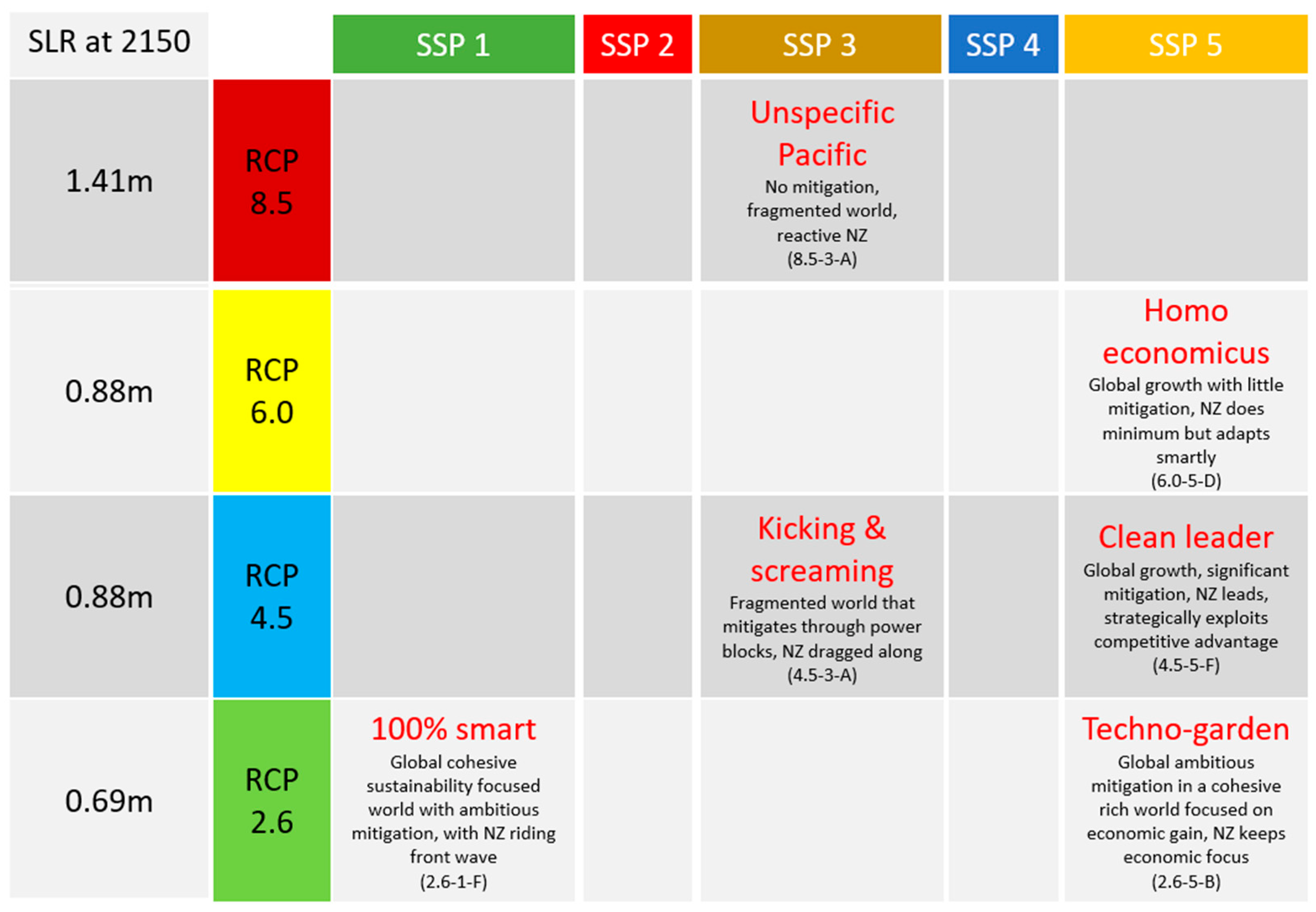
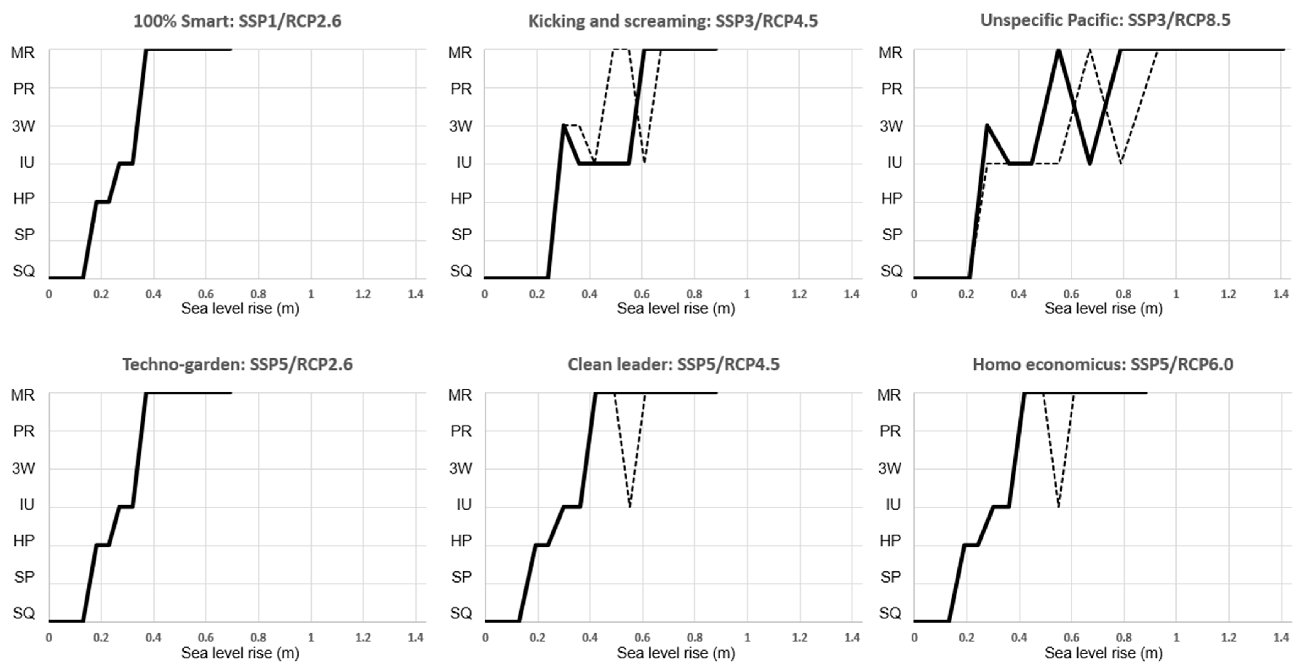
‘Kicking and screaming’ and ‘Clean leader’ are both RCP4.5, but have different SSPs (SSP3 and SSP5, respectively). Analysis of the most common pathways in each of these scenarios (Figure 3 of main paper) shows notable differences; as the RCP coding is identical for these two scenarios, these changes can only be driven by SSP.
(2)
Comparison of the most common pathways in ‘kicking and screaming’ (RCP4.5 SSP3) and ‘Unspecific Pacific’ (RCP8.5 SSP3) shows differences in both pathways selected and the timing of these pathways; as the SSP coding for these scenarios is identical, it can be inferred that RCP is the driver of these differences.
(3)
‘Homo economicus’ (RCP6.0 SSP5) and ‘Clean leader’ (RCP4.5 SSP5) show identical pathways, as RCP6.0 and RCP4.5 are coded very similarly, with only minor changes in rainfall/runoff patterns between the two RCPs; as the pathways between the two scenarios are identical, rainfall/runoff can be ruled out as a driver of pathway changes, and the rate of SLR and associated coastal inundation confirmed as the main drivers of adaptation pathway changes in these scenarios.
Storm event impacts are simulated stochastically, with sea level during storms based on water level data for Omokoroa, Tauranga [76]. The likelihood of a storm event is based on AEP, with a random-float function to ensure a randomised distribution of event occurrence. Hazards are counted as an impact event on the impact counter when: inundation occurs, with sea water above ground level, or groundwater level is above ground level. Two indirect hazards (erosion and inundation) do not directly raise the impact counter of a patch but can render patches more susceptible to inundation or groundwater intrusion. Erosion gradually reduces the elevation of affected patches. High volumes of rainfall/runoff can lead to groundwater level being above ground level. The likelihood and timing of storm events are not influenced by RCP due to insufficient data, and so the size of storm events does not change over time. However, sea-level rise makes high impact storm events increasingly likely, as surge height is added to sea level to give the total water level during storms. Sea level also influences groundwater level and the likelihood of a 1%, 2% or 3% AEP storm impact (which drives erosion), while maximum rainfall/runoff volumes are coded based on RCP; hence, all hazards in MHCABM are driven by RCP.
The number of buildings in MHCABM is set up to represent the Mount North-Omanu area of Tauranga but downscaled; one building in the model represents ten in the actual system. This downscaling was carried out to speed up model run-time, which in NetLogo is largely dependent on the number of agents in a model. Buildings may be impacted by hazard events depending on their elevation above mean sea level, the groundwater level in their patch, and the timing and magnitude of storm impact events.
A mixed cost apportionment regime was chosen based on the results of Allison et al., [53], with half the costs of adaptation falling on the affected individual, and half covered by rates and taxes. Only the most deprived dwellings (9/9 on the NZ individual index of deprivation) are unable to pay their contribution and so are unable to adapt to hazards. Mixed cost apportionment is the most likely method of climate change adaptation [6], hence is a sensible choice.
MHCABM spatially intersects hazard events with the buildings in the impact zone of these events, and thus shows exposure leading to consequence; risk is generally calculated as (exposure * likelihood). For example, the number of houses exposed to an event of a certain size, combined with their ability/inability to respond to an event, leads to the consequence of the exposure. MHCABM can also be used to calculate economic risk by considering the value of buildings exposed to an event, rather than the number of buildings exposed. The Monte Carlo simulations, and the probability distributions they produce, extricate risk from exposure by determining the likelihood of an event or other system change. This method allows for the quantification of risk for any given event in any given year, within the constraints of the simplified version of reality simulated in the model.
The coded DAPP submodel instigates societal adaptation responses to hazard impacts. The seven indicators (Table 1 of main paper) are monitored at each timestep, and if they meet or exceed a trigger value the process discussed in Appendix B is followed, where an action is selected, a lead time established, and eventually a change of action and pathway occurs.

Appendix B. Methodological Overview

This research establishes a mixed-methods approach combining qualitative and quantitative methods for developing a shared system understanding between the researchers involved, then developing and testing a model to investigate system form and function and which is comprehensible to researchers from a diverse array of disciplinary backgrounds. It builds on the transdisciplinary modelling methodology developed by Allison [41]. This section presents the methods used to scope, develop, test and document MHCABM: workshops, expert judgement, face validity, Dynamic Adaptive Pathways Planning (DAPP), agent-based modelling (ABM), scenario analysis, Monte Carlo analyses, the ODD protocol and structured walkthroughs.
Workshops are useful at the early stages of research for developing a shared system understanding and problem definition [41,79]. In later stages, workshops are a common approach of determining the accessibility and acceptability of model outputs to researchers and stakeholders at the model testing stage [41,80].
Two commonly-used techniques in workshops are expert judgement and face validity. We distinguish expert judgement, where a group of researchers/stakeholders are brought together in a discursive process, from expert elicitation, where a structured and replicable framework to knowledge acquisition is applied. Face validity is a specific type of expert judgement where, in the later stages of a research program, experts collectively consider whether a model and its behaviour are reasonable [70].
Development of a DAPP requires expert judgement to determine the indicators, system states, and adaptation thresholds to be avoided, along with identifying realistic possible responses to these indicators in the form of actions and options. DAPP development commonly occurs in a workshop setting due to the need for fluid discussion of the system and to negotiate potential responses to hazards [25]. In other situations, a DAPP may have already been developed for a community, infrastructure assets, or a region.
Determining the initial values for signals and triggers is generally carried out via expert judgement and/or stakeholder input as these values are necessarily system-specific [17,33,81]. However, once developed, models can be used as optimisation tools to determine the most likely time that signals, triggers and adaptation thresholds will occur through an iterative series of Monte Carlo simulation analyses. Through determining the distribution and mean timing of signals, triggers and adaptation thresholds, more timely adaptation can be implemented by ensuring that the values for signals and triggers are appropriate to avoid the adaptation threshold in question.
Two workshop discussions were held among the authors to develop a DAPP for the Tauranga case study. The first considered a range of indicators derived from Lawrence et al.’s [25] work looking at developing signals and triggers in a New Zealand context and assessed their potential applicability to the case study. The DAPP makes use of eight indicators from financial, social, psychological, hazard and policy fields (Table 1 of main paper) and is driven by RCP [19,82] and shared socio-economic pathway (SSP) [20].
Each STAT group uses the same indicator for signals, triggers and adaptation thresholds, with different values for each, and runs as an independent entity without influence from other STAT groups. A signal becomes active, followed by a trigger and subsequently the adaptation threshold is breached; these can happen separately or at the same time, depending on the driver of the indicator. For example, a large storm event can make all components of a STAT group activate simultaneously (signal and trigger become active and adaptation threshold is breached). Multiple triggers can become active at once for the same reasons, so a ‘multiple active triggers’ (MAT) STAT group was built into the model. If MAT is activated, a new action selection process begins, as would happen in a real decision-making situation when multiple triggers are active, to check whether the action selected by the first trigger will be suitable. Under MAT, a choice is made between options C, D and F, with the caveat that the current adaptation action cannot be selected. As an example, if the current action is C then the choice is made between options D and F.
The second workshop discussion considered the values for a signal, trigger and adaptation threshold for each of the indicators and plausible actions associated with each trigger. A suite of options was developed (Table 2 of main paper) and their applicability for each trigger considered. Each trigger was allocated a suite of plausible options and the next action (pathway) is selected from the options based on pre-determined probabilities determined during the second workshop. STAT H has no signal or adaptation threshold, only a trigger; this trigger becomes active when any other STAT group selects option ‘F—Prepare to Retreat’ as its action. As with the MAT STAT group, the current adaptation option cannot be selected by any trigger, as that would constitute no change in action or pathway.
ABM is a well-established approach for simulating the interactions between people and the environment [83,84,85,86] and is the most common approach for modelling with stakeholders [87,88]. ABM is particularly useful for improving system understanding [84,85], for investigating the actions of autonomous actors on system form and function and investigating interactions between actors [44,45]. ABMs are spatially explicit, which allows researchers to investigate the interactions of processes discrete in space and time [84,89]. ABM can help to illuminate non-linear dynamics in complex systems, making it a particularly useful approach when exploring possible impacts of decision-making on coastal communities. ABM is known for the ease in which new variables and interactions can be coded into a model, and the models produced can quickly become irredeemably complicated [41,84]. Care must be taken to only include the variables and interactions required to simulate system form and function to the extent required [41,90].
Scenario analysis involves the simulation of plausible alternate future states that may change and evolve over time. The approach of selecting already-existing scenarios is well established in modelling and simulation, for example the common use of the IPCC’s RCP and SSP scenarios [19,20]. The scenarios can be fully interrogated through running large numbers of simulations to identify the full range of potential system states each scenario can generate. Monte Carlo analysis is one such computational technique that makes use of stochastic processes to analyse risk. It consists of running large numbers (usually 1000+) of iterations of the same scenario to identify the range of possible system states that scenarios can generate and to derive probability distributions [91,92].
MHCABM gives users a choice of six scenarios, developed by Frame et al., [52] and expanded by Lawrence et al. [25]. The scenarios fit within an SSP-RCP matrix and each show a different potential future for New Zealand. The five interacting hazards drive overall system change over the period 2010 to 2150. MHCABM demonstrates a process of choosing pathways and moving through a DAPP over time, showing how a community may potentially move through the decision-making process given the conditions simulated in the model. Users can choose to run the model with a choice of six non-player characters adapted from Blackett et al. [93], each with their own preferred suite of options in response to each trigger. This paper uses the default selection of no character, allowing the model to select DAPP options for each trigger that were developed based on expert judgement.
Monte Carlo analyses were run on the six scenarios within an exploratory modelling process [94] to identify the most common DAPP pathway at each timestep for each scenario. Additionally, mean timings and distributions of each response variable (pathway, signal, trigger and adaptation threshold) were identified for each simulation group. With the intention of demonstrating model utility for decision-making this research uses 2500 iterations per calibration, increased from 1000 in the previous work [53] when MHCABM was being used in a purely exploratory manner.
Following the robust decision-making approach of presenting ‘possibilities’ rather than ‘probabilities’, and the known issues with using statistical significance to interpret model results set out in White et al. [95], we suggest only using statistical testing to confirm or refute significant differences between scenarios, rather than to suggest the likelihood of any given scenario occurring. If there is a demonstrable need to identify statistically significant differences between scenarios, we suggest comparison of scenarios via selected response variables using generalised linear models (GLMs), with a family-wise error rate correction (Holm–Bonferroni) to counteract the problem of multiple comparisons, in R Project for Statistical Computing Software (R) [96], as per Allison [41,43].
To minimise the issue of non-standardised/non-replicable model descriptions, the Overview, Design concepts and Detail (ODD) Protocol was introduced by Grimm et al., [71,72]. The ODD protocol is an increasingly common format for documenting and presenting ABMs, particularly human–environment systems models (e.g., [97,98]).
Structured walkthroughs are a form of face validity that involve a model and code being formally reviewed by a group of peers; the code can be reviewed either line-by-line or operation by operation [70]. Structured walkthroughs are an increasingly common method of model testing and are a proven method of testing model robustness and comprehensibility [41,70]. An ODD protocol description of a model can facilitate the structured walkthrough by presenting the model in a standardised way.
A structured walkthrough of model code and function was led by the model developer (AA) and undertaken with the other researchers in this project. A formalised, written version of the structured walkthrough is presented in Appendix A.1.
MHCABM, with its rule-based code structure and open-source platform, is flexible enough that it could be explicitly applied to a place if given a GIS interface, as is possible with NetLogo. MHCABM uses a patch-based spatial system, with information from hazard maps converted into point data and each point representing one patch. The size of the system that a DAPP can be applied to is flexible, with some being designed for use in small communities [99] and others for much larger geographic areas [100].

Notes

1
We define desirability in the context of development/intensification on any given spatial area unit in the model with respect to sea levels. It is based on land being above high tide level, the value and age of property in the location, and the record of hazard impacts on the location. Any spatial area unit with a desirability value above the minimum threshold can have a house or business developed on it, if a ‘person’ agent at that location chooses to do so.
2
Freshwater, wastewater and stormwater provision.
3
House loans in New Zealand require insurance to be available and increasingly insurance companies are seeing sea-level rise as a foreseeable and therefore an uninsurable cause of damage.

References

  1. Hinkel, J.; Lincke, D.; Vafeidis, A.T.; Perrette, M.; Nicholls, R.J.; Tol, R.S.J.; Marzeion, B.; Fettweis, X.; Ionescu, C.; Levermann, A. Coastal flood damage and adaptation costs under 21st century sea level rise. Proc. Natl. Acad. Sci. USA 2014, 111, 3292–3297. [Google Scholar] [CrossRef] [PubMed]
  2. Nicholls, R.J. Planning for the impacts of sea level rise. Oceanography 2011, 24, 144–157. [Google Scholar] [CrossRef]
  3. Nicholls, R.J.; Hanson, S.; Herweijer, C.; Patmore, N.; Hallegatte, S.; Corfee-Mordlot, J.; Chateau, J.; Muir-Wood, R. Ranking Port Cities with High Exposure and Vulnerability to Climate Extremes: Exposure Estimates; Environment Working Paper No. 1; Organization for Economic Co-Operation and Development: Paris, France, 2008.
  4. Rouse, H.L.; Bell, R.G.; Lundquist, C.J.; Blackett, P.E.; Hicks, D.M.; King, D.N. Coastal adaptation to climate change in Aotearoa-New Zealand. N. Z. J. Mar. Freshw. Res. 2016, 51, 183–222. [Google Scholar] [CrossRef]
  5. Iorns, C.; Watts, J. Adaptation to Sea Level Rise: Local Government Liability Issues; Deep South National Science Challenge: Wellington, New Zealand, 2019; 234p. [Google Scholar]
  6. Boston, J.; Lawrence, J. Funding Climate Change Adaptation, the case for a new policy framework. Policy Q. 2018, 14, 40–49. [Google Scholar] [CrossRef]
  7. Storey, B.; Noy, I. Insuring property under climate change. Policy Q. 2017, 13, 68–74. [Google Scholar] [CrossRef]
  8. Lawrence, J.; Bell, R.; Blackett, P.; Stephens, S.; Allan, S. National guidance for adapting to hazards and sea-level rise: Anticipating change, when and how to change pathway. Environ. Sci. Policy 2018, 82, 100–107. [Google Scholar] [CrossRef]
  9. Stephens, S. The Effect of Sea-Level Rise on the Frequency of Extreme Sea Levels in New Zealand; Prepared by NIWA for the Parliamentary Commissioner for the Environment; Parliamentary Commission for the Environment: Wellington, New Zealand, 2015; 48p.
  10. Marchau, V.A.J.W.; Walker, W.E.; Bloemen, P.J.T.M.; Popper, S.W. Introduction. In Decision Making under Deep Uncertainty. From Theory to Practice; Marchau, V.A.W.J., Walker, W.E., Bloemen, P.J.T.M., Popper, S.W., Eds.; Springer Open: Cham, Switzerland, 2019; pp. 1–21. [Google Scholar]
  11. Stephens, S.A.; Bell, R.G.; Lawrence, J. Applying principles of uncertainty within coastal hazard assessments to better support coastal adaptation. J. Mar. Sci. Eng. 2017, 5, 40. [Google Scholar] [CrossRef]
  12. Sunstein, C.R. Cost-benefit analysis and the environment. Ethics 2005, 115, 351–385. [Google Scholar] [CrossRef]
  13. Konidari, P.; Mavrakis, D. A multi-criteria evaluation method for climate change mitigation policy instruments. Energy Policy 2021, 50, 229–241. [Google Scholar] [CrossRef]
  14. Stroombergen, A.; Lawrence, J. A novel illustration of real options analysis to address the problem of probabilities under deep uncertainty and changing climate risk. Clim. Risk Manag. 2022, 38, 100458. [Google Scholar] [CrossRef]
  15. Lempert, R.J. Chapter 2: Robust Decision-Making. In Decisionmaking under Deep Uncertainty: From Theory to Practice; Marchau, V., Walker, W., Bloeman, P., Popper, S.W., Eds.; Springer: Cham, Switzerland, 2019; pp. 23–52. [Google Scholar]
  16. Haasnoot, M.; Warren, A.; Kwakkel, J.H. Dynamic Adaptive Policy Pathways (DAPP). In Decision-Making under Deep Uncertainty: From Theory to Practice; Marchau, V.A.W.J., Walker, W.E., Bloemen, P.J.T.M., Popper, S.W., Eds.; Springer: Cham, Switzerland, 2019; pp. 71–92. [Google Scholar]
  17. Walker, W.E.; Haasnoot, M.; Kwakkel, J.H. Adapt or perish: A review of planning approaches for adaptation under deep uncertainty. Sustainability 2013, 5, 955–979. [Google Scholar] [CrossRef]
  18. Pörtner, H.-O.; Roberts, D.C.; Poloczanska, E.S.; Mintenbeck, K.; Tignor, M.; Alegría, A.; Craig, M.; Langsdorf, S.; Löschke, S.; Möller, V.; et al. (Eds.) Summary for Policymakers. In Climate Change 2022: Impacts, Adaptation, and Vulnerability; Contribution of Working Group II to the Sixth Assessment Report of the Intergovernmental Panel on Climate Change 2022a; Cambridge University Press: Cambridge, UK; New York, NY, USA, 2022; pp. 3–33. [Google Scholar]
  19. IPCC. Summary for Policymakers. In Climate Change 2014: Mitigation of Climate Change; Contribution of Working Group III to the Fifth Assessment Report of the Intergovernmental Panel on Climate Change; Edenhofer, O., Pichs-Madruga, R., Sokona, Y., Farahani, E., Kadner, S., Seyboth, K., Adler, A., Baum, I., Brunner, S., Eickemeier, P., et al., Eds.; Cambridge University Press: Cambridge, UK; New York, NY, USA, 2014. [Google Scholar]
  20. Riahi, K.; van Vuuren, D.P.; Kriegler, E.; Edmonds, J.; O’Neill, B.C.; Fujimori, S.; Bauer, N.; Calvin, K.; Dellink, R.; Fricko, O.; et al. The Shared Socioeconomic Pathways and their energy, land use and greenhouse gas emissions implications: An overview. Glob. Environ. Chang. 2017, 42, 153–168. [Google Scholar] [CrossRef]
  21. Levermann, A.; Clark, P.U.; Marzeion, B.; Milne, G.A.; Pollard, D.; Radic, V.; Robinson, A. The multimillennial sea-level commitment of global warming. Proc. Natl. Acad. Sci. USA 2013, 110, 13745–13750. [Google Scholar] [CrossRef] [PubMed]
  22. Cooley, S.; Schoeman, D.; Bopp, L.; Boyd, P.; Donner, S.; Ghebrehiwet, D.Y.; Ito, S.-I.; Kiessling, W.; Martinetto, P.; Ojea, E.; et al. Chapter 3: Oceans and Coastal Ecosystems and Their Services. In Climate Change 2022: Impacts, Adaptation and Vulnerability; Working Group II Contribution to the Sixth Assessment Report of the Intergovernmental Panel on Climate Change; Cambridge University Press: Cambridge, UK; New York, NY, USA, 2022; pp. 295–408. [Google Scholar]
  23. Ministry for the Environment. Preparing for Coastal Change; A Summary of Coastal Hazards and Climate Change Guidance for Local Government; Bell, R., Lawrence, J., Allan, S., Blackett, P., Stephens, S., Eds.; Ministry for the Environment: Wellington, New Zealand, 2017; Publication ME 1335.
  24. Haasnoot, M.; van’t Kluster, S.; van Alphen, J. Designing a monitoring system to detect signals to adapt to uncertain climate change. Glob. Environ. Chang. 2018, 52, 273–285. [Google Scholar] [CrossRef]
  25. Lawrence, J.; Bell, R.; Blackett, P.; Stephens, S.; Collins, D.; Craddock-Henry, N.; Hardcastle, M. Supporting Decision Making through Adaptive Tools in a Changing Climate, Practice Guidance on Signals and Triggers; The Deep South National Science Challenge; Victoria University of Wellington: Wellington, New Zealand, 2020. [Google Scholar]
  26. Haasnoot, M.; Kwakkel, J.H.; Walker, W.E.; ter Maat, J. Dynamic adaptive policy pathways: A method for crafting robust decisions for a deeply uncertain world. Glob. Environ. Chang. 2013, 23, 485–498. [Google Scholar] [CrossRef]
  27. Islam, M.M.; Rahman, M.A.; Khan, M.S.; Mondal, G.; Khan, M.I. Transformational adaptation to climatic hazards: Insights from mangroves-based coastal fisheries dependent communities of Bangladesh. Mar. Policy 2021, 128, 104475. [Google Scholar] [CrossRef]
  28. Zagaria, C.; Schulp, C.J.E.; Zavalloni, M.; Viaggi, D.; Verburg, P.H. Modelling transformational adaptation to climate change among crop farming systems in Romagna, Italy. Agric. Syst. 2021, 188, 103024. [Google Scholar] [CrossRef]
  29. Kates, R.W.; Travis, W.R.; Wilbanks, T.J. Transformational adaptation when incremental adaptations to climate change are insufficient. Proc. Natl. Acad. Sci. USA 2012, 109, 7156–7161. [Google Scholar] [CrossRef]
  30. Kool, R.; Lawrence, J.; Drews, M.; Bell, R. Preparing for Sea-Level Rise through Adaptive Managed Retreat of a New Zealand Stormwater and Wastewater Network. Infrastructures 2020, 5, 92. [Google Scholar] [CrossRef]
  31. Haasnoot, M.; Lawrence, J.; Magnan, A.K. Pathways to coastal retreat. Science 2021, 372, 1287–1290. [Google Scholar] [CrossRef]
  32. Walker, W.E.; Marchau, V.A.W.J.; Kwakkel, J.H. Dynamic Adaptive Planning. In Decision Making under Deep Uncertainty; Marchau, V.A.W.J., Walker, W.E., Bloemen, P.J.T.M., Popper, S.W., Eds.; Springer: Cham, Switzerland, 2019; pp. 53–69. [Google Scholar]
  33. Werners, S.; Pfenniger, S.; van Slobbe, E.; Haasnoot, M.; Kwakkel, J.H.; Swart, R.J. Thresholds, tipping and turning points for sustainability under climate change. Curr. Opin. Environ. Sustain. 2013, 5, 334–340. [Google Scholar] [CrossRef]
  34. Stephens, S.A.; Bell, R.G.; Lawrence, J. Developing signals to trigger adaptation to sea-level rise. Environ. Res. Lett. 2018, 13, 104004. [Google Scholar] [CrossRef]
  35. Dafermos, Y.; Nikolaidi, M.; Galanis, G. Climate Change, Financial Stability and Monetary Policy. Ecol. Econ. 2018, 152, 219–234. [Google Scholar] [CrossRef]
  36. Climate Change Adaptation Technical Working Group. Adapting to Climate Change in New Zealand; Ministry for the Environment: Wellington, New Zealand, 2017; ISBN 978-1-98-852527-3.
  37. Gasper, R.; Blohm, A.; Ruth, M. Social and economic impacts of climate change on the urban environment. Curr. Opin. Environ. Sustain. 2011, 3, 150–157. [Google Scholar] [CrossRef]
  38. Tol, R. The Economic Impact of Climate Change; ESRI Working Paper, No. 255; The Economic and Social Research Institute (ESRI): Dublin, Ireland, 2008. [Google Scholar]
  39. Kwakkel, J.H.; Haasnoot, M.; Walker, W.E. Comparing Robust Decision-Making and Dynamic Adaptive Policy Pathways for model-based decision support under deep uncertainty. Environ. Model. Softw. 2016, 86, 168–183. [Google Scholar] [CrossRef]
  40. Kwakkel, J.H.; Haasnoot, M.; Walker, W.E. Developing dynamic adaptive policy pathways: A computer-assisted approach for developing adaptive strategies for a deeply uncertain world. Clim. Chang. 2015, 132, 373–386. [Google Scholar] [CrossRef]
  41. Allison, A.E.F. Developing a Methodology for Transdisciplinary Modelling of Complex Human-Environment Systems. Ph.D. Thesis, The University of Auckland, Auckland, New Zealand, 2020; 242p. unpublished. [Google Scholar]
  42. O’Sullivan, D.; Millington, J.; Perry, G.; Wainwright, J. Agent-Based Models—Because They’re Worth It? In Agent-Based Models of Geographical Systems; Heppenstall, A.J., Crooks, A., See, L.M., Batty, M., Eds.; Springer: Dordrecht, The Netherlands, 2012; 138p. [Google Scholar]
  43. Allison, A.E.F.; Dickson, M.E.; Fisher, K.T.; Thrush, S.F. Communicating drivers of environmental change through transdisciplinary human-environment modelling. Earth’s Future 2021, 9, e2020EF001918. [Google Scholar] [CrossRef]
  44. McNamara, D.E.; Keeler, A. A coupled physical and economic model of the response of coastal real estate to climate risk. Nat. Clim. Chang. 2013, 3, 559–562. [Google Scholar] [CrossRef]
  45. Luo, M.; Opaluch, J.J.; Anderson, J.L.; Schnier, K. Managing the Intentional Introduction of Nonnative Species. In Oysters: Physiology, Ecological Distribution and Mortality; Qin, J.G., Ed.; Flinders University: Adelaide, Australia, 2012; pp. 101–145. [Google Scholar]
  46. Lawrence, J.; Bell, R.; Stroombergen, A. A Hybrid Process to Address Uncertainty and Changing Climate Risk in Coastal Areas Using Dynamic Adaptive Pathways Planning, Multi-Criteria Decision Analysis & Real Options Analysis: A New Zealand Application. Sustainability 2019, 11, 406. [Google Scholar] [CrossRef]
  47. Deep South National Science Challenge, Sea Level Rise and River Flooding: Flood Risk under Climate Change. 2019. Available online: https://deepsouthchallenge.co.nz/sea-level-rise-and-river-flooding-flood-risk-under-climate-change/ (accessed on 16 November 2022).
  48. Aerts, J.C.J.H. Integrating agent-based approaches with flood risk models: A review and perspective. Water Secur. 2020, 2020, 100076. [Google Scholar] [CrossRef]
  49. Haer, T.; Botzen, W.J.W.; Aerts, J.C.J.H. Advancing disaster policies by integrating dynamic adaptive behaviour in risk assessments using an agent-based modelling approach. Environ. Res. Lett. 2019, 14, 044022. [Google Scholar] [CrossRef]
  50. Allison, A.E.F. Multi-Hazard Coastal Agent-Based Model (MHCABM) (version 1.0.0), CoMSES, Published 5 August 2021. Available online: https://www.comses.net/codebases/5d9768df-97ae-4994-8517-6af877d8b9b5/releases/1.0.0/ (accessed on 25 November 2022).
  51. Atkinson, J.; Salmond, C.; Crampton, P. NZDep2013 Index of Deprivation; University of Otago: Dunedin, New Zealand, 2014. [Google Scholar]
  52. Frame, B.; Lawrence, J.; Ausseil, A.-G.; Reisinger, A.; Daigneault, A. Adapted global shared socio-economic pathways for national and local scenarios. Clim. Risk Manag. 2018, 21, 39–51. [Google Scholar] [CrossRef]
  53. Allison, A.E.F.; Stephens, S.; Blackett, P.; Jozaei, J.; Lawrence, J.; Dickson, M.; Matthews, Y. Who Pays for Climate Change Adaptation? Investigating RCP, SSP and Cost Apportionment Impacts Using a Simple Multi-Hazard Risk Interaction Model. In Proceedings of the Australasian Coasts & Ports Conference 2021, Christchurch, New Zealand, 30 November–3 December 2021; pp. 76–82. [Google Scholar]
  54. Ministry for the Environment. Interim Guidance on the Use of New Sea-Level Rise Projections; Ministry for the Environment: Wellington, New Zealand, 2022.
  55. Lawrence, J.; Boston, J.; Bell, R.; Olufson, S.; Kool, R.; Hardcastle, M.; Stroombergen, A. Implementing pre-emptive managed retreat: Constraints and novel insights. Curr. Clim. Chang. Rep. 2020, 6, 66–80. [Google Scholar] [CrossRef]
  56. Ministry of Business. Innovation and Employment 2004 Building Act. New Zealand Government Public Act 2004. No. 72. Available online: http://legislation.govt.nz/act/public/2004/0072/latest/DLM306036.html (accessed on 25 November 2022).
  57. Ministry for the Environment. Resource Management Act; Ministry for the Environment: Wellington, New Zealand, 1991.
  58. NZ Searise. Local Vertical Land Movement Projections. 2022. Available online: https://www.searise.nz (accessed on 26 May 2022).
  59. Lawrence, J.; Allan, S.; Clarke, L. Inadequacy Revealed and the Transition to Adaptation as Risk Management in New Zealand. Front. Clim. 2021, 3, 734726. [Google Scholar] [CrossRef]
  60. PCE. Preparing New Zealand for Rising Seas: Certainty and Uncertainty. Parliamentary Commissioner for the Environment. 2015. Available online: https://www.pce.parliament.nz/media/1390/preparing-nz-for-rising-seas-web-small.pdf (accessed on 25 November 2022).
  61. Lawrence, J.; Mackey, B.; Chiew, F.; Costello, M.J.; Hennessy, K.; Lansbury, N.; Nidumolu, U.B.; Pecl, G.; Rickards, L.; Tapper, N.; et al. Australasia. In Climate Change 2022: Impacts, Adaptation, and Vulnerability; Contribution of Working Group II to the Sixth Assessment Report of the Intergovernmental Panel on Climate Change; Pörtner, H.-O., Roberts, D.C., Tignor, M., Poloczanska, E.S., Mintenbeck, K., Alegría, A., Craig, M., Langsdorf, S., Löschke, S., Möller, V., et al., Eds.; Cambridge University Press: Cambridge, UK; New York, NY, USA, 2022. [Google Scholar]
  62. Ministry for the Environment and Statistics New Zealand. Our Marine Environment 2019. Available online: https://environment.govt.nz/assets/publications/Files/our-marine-environment-2019.pdf (accessed on 29 January 2023).
  63. Storey, B.; Owen, S.; Zammit, C.; Noy, I. Insurance Retreat in Residential Properties from Future Sea Level Rise in Aotearoa New Zealand. CESifo Working Paper No. 10017. 2022. Available online: https://ssrn.com/abstract=4257216 (accessed on 10 January 2023).
  64. Ministry for the Environment. Coastal Hazards and Climate Change: Guidance for Local Government; Bell, R., Lawrence, J., Allan, S., Blackett, P., Stephens, S., Eds.; Ministry for the Environment Publication: Wellington, New Zealand, 2017; ME 1341.
  65. Houssou, N.L.J.; Cordero, J.D.; Bouadjio-Boulic, A.; Morin, L.; Maestripieri, N.; Ferrant, S.; Belem, M.; Peláez, J.I.; Saenz, M.; Lerigoleur, E.; et al. Synchonising histories of exposure and demography: The construction of an agent-based model of the Ecuadorian Amazon colonization and exposure to oil pollution hazards. J. Artif. Soc. Soc. Simul. 2019, 22, 1. [Google Scholar] [CrossRef]
  66. Daysh, S. Clifton to Tangoio Coastal Hazard Strategy, A Practical Case Study of Community Based Decision-Making in Hawkes Bay. In Proceedings of the RMLA Conference Presentation, Wellington, New Zealand, 26 November 2018. [Google Scholar]
  67. Jacobson, M. NZCPS Coastal Hazard Policies. Plan. Q. 2005, 24, 6–8. [Google Scholar]
  68. Lempert, R.J. Robust Decision-Making (RDM). In Decision-Making under Deep Uncertainty; Marchau, V.A.J.W., Walker, W.E., Bloemen, P.J., Popper, S.W., Eds.; Springer: Cham, Switzerland, 2019; pp. 23–51. [Google Scholar]
  69. Li, Y. Deep reinforcement learning: An overview. arXiv 2017, arXiv:1810.06339. [Google Scholar] [CrossRef]
  70. Sargent, R.G. Verification and validation of simulation models. J. Simul. 2013, 7, 12–24. [Google Scholar] [CrossRef]
  71. Grimm, V.; Berger, U.; Bastiansen, F.; Eliassen, S.; Ginot, V.; Giske, J.; GossCustard, J.; Grand, T.; Heinz, S.K.; Huse, G.; et al. A standard protocol for describing individual-based and agent-based models. Ecol. Model. 2006, 198, 115–126. [Google Scholar] [CrossRef]
  72. Grimm, V.; Berger, U.; DeAngelis, D.L.; Polhill, J.G.; Giske, J.; Railsback, S.F. The ODD protocol: A review and first update. Ecol. Model. 2010, 221, 2760–2768. [Google Scholar] [CrossRef]
  73. Statistics New Zealand. New Zealand Census. 2013. Available online: https://stats.govt.nz/census/previous-censuses/2013-census/ (accessed on 18 October 2022).
  74. Reisinger, A.; Kitching, R.L.; Chiew, F.; Hughes, L.; Newton, P.C.D.; Schuster, S.S.; Tait, A.; Whetton, P. Australasia. In Climate Change 2014: Impacts, Adaptation, and Vulnerability; Part B: Regional Aspects; Contribution of Working Group II to the Fifth Assessment Report of the Intergovernmental Panel on Climate Change; Barros, V.R., Field, C.B., Dokken, D.J., Mastrandrea, M.D., Mach, K.J., Bilir, T.E., Chatterjee, M., Ebi, K.L., Estrada, Y.O., Genova, R.C., et al., Eds.; Cambridge University Press: Cambridge, UK; New York, NY, USA, 2014; pp. 1371–1438. [Google Scholar]
  75. Carey-Smith, T.; Dean, S.; Vial, J.; Thompson, C. Changes in precipitation extremes for New Zealand: Climate model predictions. Weather Clim. 2010, 30, 23–48. [Google Scholar] [CrossRef]
  76. Reeve, G.; Stephens, S.; Wadhwa, S. Tauranga Harbour Inundation Modelling 2019; NIWA Climate Report: 2018269HN; NIWA: Hamilton, New Zealand, 2019. [Google Scholar]
  77. Bitan, M.; Zviely, D. Sand beach nourishment: Experience from the Mediterranean Coast of Israel. J. Mar. Sci. Eng. 2020, 8, 273. [Google Scholar] [CrossRef]
  78. Statistics New Zealand. Trending Topics—Housing. 2017. Available online: https://www.stats.govt.nz/assets/Reports/Trending-topics-Housing/trending-topics-housing.pdf (accessed on 18 October 2022).
  79. Faber, J.H.; Marshall, S.; van den Brink, P.J.; Maltby, L. Priorities and opportunities in the application of the ecosystem services concept in risk assessment for chemicals in the environment. Sci. Total Environ. 2019, 651, 1067–1077. [Google Scholar] [CrossRef]
  80. Baier, R.R.; Jutkowicz, E.; Mitchell, S.L.; McCreedy, E.; Mor, V. Readiness assessment for pragmatic trials (RAPT): A model to assess the readiness of an intervention for testing in a pragmatic trial. Med. Res. Methodol. 2019, 19, 156. [Google Scholar] [CrossRef] [PubMed]
  81. Tariq, A.; Lempert, R.J.; Riverson, J.; Schwartz, M.; Berg, N. A climate stress test of Los Angeles’ water quality plans. Clim. Chang. 2017, 144, 625–639. [Google Scholar] [CrossRef]
  82. van Vuuren, D.P.; Edmonds, J.; Kainuma, M.; Riahi, K.; Thompson, A.; Hibbard, K.; Hurtt, G.C.; Kram, T.; Krey, V.; Lamarque, J.-F.; et al. The representative concentration pathways: An overview. Clim. Chang. 2011, 109, 5–31. [Google Scholar] [CrossRef]
  83. Schlüter, M.; McAllister, R.R.J.; Alinghaus, R.; Bunnefeld, N.; Eisenack, K.; Hölker, F.; Milner-Gulland, E.J.; Müller, B. New Horizons for Managing the Environment: A Review of Coupled Social-Ecological Systems Modeling. Nat. Resour. Model. 2012, 25, 219–272. [Google Scholar] [CrossRef]
  84. Kelly, R.A.; Jakeman, A.J.; Barreteau, O.; Bursuk, M.E.; Elsawah, S.; Hamilton, S.H.; Hendriksen, H.J.; Kuikka, S.; Maier, H.R.; Rizzoli, A.E.; et al. Selecting among five common modelling approaches for integrated environmental assessment and management. Environ. Model. Softw. 2013, 47, 159–181. [Google Scholar] [CrossRef]
  85. Bousquet, F.; Le Page, C. Multi-agent simulations and ecosystem management: A review. Ecol. Model. 2004, 176, 313–332. [Google Scholar] [CrossRef]
  86. Lempert, R.J. A new decision sciences for complex systems. Proc. Natl. Acad. Sci. USA 2002, 99 (Suppl. S3), 7309–7313. [Google Scholar] [CrossRef]
  87. Seidl, R. A functional-dynamic reflection on participatory processes in modeling projects. Ambio 2015, 44, 750–765. [Google Scholar] [CrossRef] [PubMed] [Green Version]
  88. Simon, C.; Etienne, M. A companion modelling approach applied to forest management planning. Environ. Model. Softw. 2010, 25, 1371–1384. [Google Scholar] [CrossRef]
  89. Voinov, A.; Bousquet, F. Modelling with stakeholders. Environ. Model. Softw. 2010, 25, 1268–1281. [Google Scholar] [CrossRef]
  90. Allison, A.E.F.; Dickson, M.E.; Fisher, K.T.; Thrush, S.F. Dilemmas of modelling and decision-making in environmental research. Environ. Model. Softw. 2018, 99, 147–155. [Google Scholar] [CrossRef]
  91. Heijungs, R. On the number of Monte Carlo runs in comparative probabilistic LCA. Int. J. Life Cycle Assess. 2020, 25, 394–402. [Google Scholar] [CrossRef]
  92. Johnston, J.M.; McGarvey, D.J.; Barber, M.C.; Laniak, G.; Babendreier, J.; Parmar, R.; Wolfe, K.; Kraemer, S.R.; Cyterski, M.; Knightes, C.; et al. An integrated modelling framework for performing environmental assessments: Application to ecosystem services in the Albemarle-Pamlico basins (NC and VA, USA). Ecol. Model. 2011, 222, 2471–2484. [Google Scholar] [CrossRef]
  93. Blackett, P.; Davies, K.; Davies, B.; Holland, P.; Craddock-Henry, N. “Adaptive Futures” An Interactive Serious Game for Decision-Making and Coastal Hazards; NIWA Client Report 2019328HN; NIWA: Hamilton, New Zealand, 2019. [Google Scholar]
  94. Moallemi, E.A.; Kwakkel, J.; de Haan, F.J.; Bryan, B.A. Exploratory modelling for analyzing coupled human-natural systems under uncertainty. Glob. Environ. Chang. 2020, 65, 102186. [Google Scholar] [CrossRef]
  95. White, J.W.; Rassweiler, A.; Samhouri, J.F.; Stier, A.C.; White, C. Ecologists should not use statistical significance tests to interpret simulation model results. Oikos 2013, 123, 385–388. [Google Scholar] [CrossRef]
  96. R Core Team. R: A Language and Environment for Statistical Computing; R Foundation for Statistical Computing: Vienna, Austria, 2017; Available online: https://www.R-project.org/ (accessed on 25 November 2022).
  97. Pliknyas, D.; Laužikas, R.; Sakalauskas, L.; Miliauskas, A.; Dulskis, V. Agent-Based Simulation of Cultural Events on Social Capital Dynamics. In Intelligent Systems and Applications; Advances in Intelligent Systems and Computing; Bi, Y., Bhatia, R., Kapoor, S., Eds.; Springer: Cham, Switzerland, 2020; Volume 1037. [Google Scholar]
  98. Suárez-Muñoz, M.; Bonet-García, F.; Hódar, J.; Herrero, J.; Tanase, M.; Torres-Muros, L. INSTAR: An agent-based model that integrates existing knowledge to simulate the population dynamics of a forest pest. Ecol. Model. 2019, 411, 108764. [Google Scholar] [CrossRef]
  99. Blackett, P.; FitzHerbert, S.; Luttrell, J.; Hopmans, T.; Lawrence, H.; Colliar, J. Marae-opoly: Supporting localised Māori climate adaptation decisions with serious games in Aotearoa New Zealand. Sustain. Sci. 2021, 17, 415–431. [Google Scholar] [CrossRef]
  100. Haasnoot, M.; Schellekens, J.; Middlekoop, H.; Kwadijk, J.C.J. Transient scenarios for robust climate change adaptation illustrated for water management in the Netherlands. Environ. Res. Lett. 2015, 10, 105008. [Google Scholar] [CrossRef] [Green Version]
Figure 1. Example DAPP ‘metro map’ showing a range of actions available (left axis) and potential transfer points (circles) between actions (coloured lines). Some actions (e.g., actions A, B and D) will reach adaptation thresholds faster than others (e.g., actions C and E) and therefore have shorter life spans. We tested the lifetimes of different actions by integrating a DAPP into the model. Each coloured line represents a different adaptive action.
Jmse 11 00343 g001
Figure 2. An example sequence of events under climate change. DAPP uses the trigger to instigate a change in action to avoid the adaptation threshold occurring.
Jmse 11 00343 g002
Figure 3. SSP/RCP Matrix showing six plausible future scenarios for New Zealand. Reproduced from Allison et al. [53]; with permission from Engineers Australia, New Zealand Coastal Society, and PIANC 2021; adapted from Lawrence et al. [25].
Jmse 11 00343 g003
Figure 4. Most common adaptation action for each scenario with RSLR on the X axis and adaptation action on the Y axis. Solid line indicates the most common pathway; dotted line indicates when another action is at least 90% as likely as the most common pathway to occur at that timestep—a ‘second-most common pathway’. Adaptive actions are shown in Figure 5.
Jmse 11 00343 g004
Figure 5. Adaptation pathway map representing the range of viable simulated pathways (i.e., that avoid adaptation thresholds) across all six SSP/RCP scenarios, based on the approximate RSLR value at which pathway changes are instigated. Unlike Figure 2, the X axis shows the timing of pathway changes based on RSLR, which is the main instigator of pathway change and which varies across scenarios. Each coloured line represents a different adaptive action.
Jmse 11 00343 g005
Figure 6. Activation time of signals, triggers and adaptation thresholds for the seven indicator variables. For this and Figure 7, Y axis shows percentage of active signals, triggers and adaptation thresholds out of 2500 Monte Carlo simulations for each SSP/RCP scenario, X axis shows level of RSLR. Blue line indicates active signals, green line indicates active triggers, orange line indicates adaptation thresholds breached. ‘K & S’ is scenario Kicking and screaming.
Jmse 11 00343 g006
Figure 7. Activation time of signals, triggers and adaptation thresholds for the seven indicator variables without implementation of DAPP.
Jmse 11 00343 g007
Table 1. Indicators used in MHCABM with the category of indicator they fall into, the signal, trigger and adaptation threshold values, and associated suite of triggered actions. Actions are as follows—SP: soft protection, HP: hard protection, IU: infrastructure upgrades, 3W: three waters2 upgrade, PR: preparation for active retreat, AR: active retreat.
IndicatorCategorySignal ValueTrigger ValueAdaptation Threshold ValueActions
Insurance premium or deductibles increaseFinancialMean annual insurance cost is 2.05% of net worthMean annual insurance cost is 2.2% of net worthMean annual insurance cost is 5% of net worthSP 60%,
IU: 40%
Maintenance costs increaseFinancialMean annual building maintenance cost is 2.1% of net worthMean annual building maintenance cost is 2.23% of net worthMean annual building maintenance cost is 5% of net worthIU: 60%,
PR: 40%
Aesthetic degradationSocialA seawall has been constructedFive or more seawalls have been constructed10 or more seawalls have been constructedIU: 60%,
PR: 40%
Total hazardous areaPsychological5 or more patches contain stressed or uninsurable houses10 or more patches contain stressed or uninsurable houses20 or more patches contain stressed or uninsurable houses3W: 60%,
IU: 20%,
HP: 20%
Decline in property desirabilityFinancialDesirability has fallen to 97.5% of its original valueDesirability has fallen to 95% of its original valueDesirability has fallen to 90% of its original valueHP: 60%,
IU: 40%
Number of flood eventsHazard5% of occupied patches have been impacted by one or more events since a 10-year event-free period10% of occupied patches have been impacted by one or more events since a 10-year event-free period20% of occupied patches have been impacted by one or more events since a 10-year event-free periodIU: 60%,
PR: 40%
Three waters vulnerabilityHazardRSLR reaches 10 cmRSLR reaches 20 cmRSLR reaches 30 cm3W: 60%,
IU: 40%
Preparation for active retreatPolicyN/ASelection of action PRN/AAR: 100%
Multiple active triggersPolicyN/ATwo or more triggers active simultaneouslyN/AHP: 33%
IU: 33%
PR: 33%
Table 2. Actions represented in MHCABM. The default initial action is raising floors and land elevation of a building to remove it from the coastal hazard zone as defined by the New Zealand Building Act [56]. Preparation for active retreat has no lead time as the preparation begins immediately, with a 20-year window before Active Retreat begins. During Preparation for active retreat agents respond to hazards via the action selected by the previous trigger.
AbbreviationActionAdaptation UndertakenLead Time
SQStatus QuoRaise floors and land elevationNone
SPSoft ProtectionBeach nourishment2 years
HPHard ProtectionBuild seawall4 years
IUInfrastructure upgradesRaise floors and land elevation, pumped three waters system, prevention of new builds in hazard zones via planning rule7 years
3WImproved Three WatersPumped three waters system5 years
PRPreparation for active RetreatConsultation and planningNone
ARActive RetreatActive Retreat20 years
Disclaimer/Publisher’s Note: The statements, opinions and data contained in all publications are solely those of the individual author(s) and contributor(s) and not of MDPI and/or the editor(s). MDPI and/or the editor(s) disclaim responsibility for any injury to people or property resulting from any ideas, methods, instructions or products referred to in the content.

