Article

Convolutional Neural Network Predictions for Unsteady Reynolds-Averaged Navier–Stokes-Based Numerical Simulations

by
Alvaro Abucide-Armas
1,
Koldo Portal-Porras
2,
Unai Fernandez-Gamiz
2,
Ekaitz Zulueta
1,* and
Adrian Teso-Fz-Betoño
1
1
Automatic Control and System Engineering Department, University of the Basque Country UPV/EHU, Nieves Cano 12, 01006 Vitoria-Gasteiz, Spain
2
Nuclear Engineering and Fluid Mechanics Department, University of the Basque Country UPV/EHU, Nieves Cano 12, 01006 Vitoria-Gasteiz, Spain
*
Author to whom correspondence should be addressed.
J. Mar. Sci. Eng. 2023, 11(2), 239; https://doi.org/10.3390/jmse11020239
Submission received: 16 December 2022 / Revised: 11 January 2023 / Accepted: 16 January 2023 / Published: 17 January 2023
(This article belongs to the Section Ocean Engineering)

Abstract

:
The application of computational fluid dynamics (CFD) to turbulent flow has been a considerable topic of research for many years. Nonetheless, using CFD tools results in a large computational cost, which implies that, for some applications, CFD may be unviable. To date, several authors have carried out research applying deep learning (DL) techniques to CFD-based simulations. One of the main applications of DL with CFD is in the use of convolutional neural networks (CNNs) to predict which samples will have the desired magnitude. In this study, a CNN which predicts the streamwise and vertical velocities and the pressure fields downstream of a circular cylinder for a series of time instants is presented. The CNN was trained using a signed distance function (SDF), a flow region channel (FRC) and the t-1 sample as inputs, and the ground-truth CFD data as the output. The results showed that the CNN was able to predict multiple time instants with low error rates for turbulent flows with variable input velocities to the domain.

1. Introduction

The study of turbulence in fluids has been a significant research topic for many years due to its impact on a wide variety of applications. The resolution of intricate computational fluid dynamics (CFD) problems has been made possible through the exponential advances in computing over the last few decades. Nevertheless, this still remains a constraint for product development related to applications such as aerodynamic design optimization and fluid–structure interactions [1]. Despite the fact that CFD simulations are a valuable tool for the study of turbulent flow when experimental studies are too expensive or impractical, the computational resources required by CFD simulations may become prohibitive if the geometry is too complex or if fine meshing is required. Another drawback in the application of CFD is the influence of the user during the generation of the mesh and the closure model.
In order to solve these issues, in recent years numerous authors have applied deep learning (DL) techniques to predict the approximated results of CFD simulations. For example, Tao and Sun [2], Zhang et al. [3] and Yan et al. [4] targeted aerodynamic optimization to improve the efficiency of diverse geometries through DL.
Two main approaches have been used to apply DL techniques to CFD. The first approach focuses on the reduction of the computational time required for studies which employ coarse meshes. For example, Hanna et al. [5] predicted and lowered the error of the results obtained for a coarse mesh using a DL algorithm, and Bao et al. [6] proposed a data-driven guidance framework to improve their coarse mesh modelling and simulation. In the second approach, the desired fluid characteristics are directly calculated. Through the development of a convolutional neural network (CNN), Guo et al. [7] predicted stationary flow fields around solid objects, accomplishing rapid predictions with low error rates. Ribeiro et al. [8] developed a very accurate CNN which predicts the streamwise and vertical velocities and the pressure fields for stationary fluids in the presence of different shaped geometries, and Kashefi et al. [9] also developed a CNN to obtain an approximation of the streamwise and vertical velocities and the pressure fields following slight modifications of the geometry.
Other studies have focused on the prediction of more specific flow characteristics. For example, Ling et al. [10], remarkably improved the results of CFD simulations by employing a deep neural network (DNN) for modelling the Reynolds stress tensors using Reynolds-Averaged Navier–Stokes (RANS) equations. Lee and You [11] predicted the shedding of non-stationary laminar vortices on a circular cylinder with a generative adversarial network (GAN). Liu et al. [12] and Deng et al. [13] applied DL-based techniques to the detection of impacts and vortexes, respectively.
With the exception of some studies which analyzed 3D geometries, such as Guo et al. [7] and Nowruzi et al. [14], the majority of researchers have studied 2D geometries, due to the high computational cost involved in the study of 3D geometries [15]. In order to analyze flow properties, Mohan et al. [15] created a DL-based infrastructure which reduces the geometry.
Due to the intricacy of the physics of turbulent flows, most studies have been applied to the prediction of laminar flows. Nonetheless, Fang et al. [16] predicted turbulent flows in a channel, and Thuerey et al. [17] utilized a CNN to approximate the streamwise and vertical velocities and the pressure fields of a RANS-based Spalart–Allmaras turbulence model on airfoils. Abucide-Armas et al. [18] obtained low error rates in their simulations of turbulent flows with variable inlet velocities, and Portal-Porras et al. [19] developed various network structures for the prediction of velocity fields for turbulent flows.
Time-based approaches were not considered in most of the aforementioned works. Nonetheless, CFD applications frequently require knowledge of how the evolution of the parameters and features of the fluid under study vary over the course of time. The following studies employed recurrent neural networks (RNNs) in order to analyze time evolutions in CFD applications: Agostini [20] predicted the streamwise velocity field time evolution using an autoencoder model; and King et al. [21], Gonzalez and Balajewicz [22] and Maulik et al. [23] predicted various flow properties via the employment of time-based approaches.
In this study, the proposed CNN was trained using ground-truth CFD results for different velocities inputted to the computational domain during a fixed period of time. The data included the streamwise and vertical velocities and the pressure fields. The aim was to exploit these data to train a CNN in order to predict the future states of the fluid given the initial state, by considering the dependency of a fluid’s state on its prior state. The testing took a random case from the CFD ground-truth data for the initial state, and used the previously predicted time instant for the remainder of the states. Each result was compared with the corresponding ground-truth data sample to obtain the ratio of the error at each instant.
The novelty of this study resides in the ability of our single CNN architecture to predict the vertical and streamwise velocities and the pressure fields throughout a specific number of time instants.

2. Materials and Methods

2.1. Numerical Simulations

An unsteady Reynolds Navier–Stokes (URANS) approach was adopted for the current simulations since this is the method usually employed when long term periodical oscillations in a turbulent flow are investigated. The URANS Equations were obtained using the following procedure. The Navier–Stokes Equations for incompressible flow were time-filtered according to Equation (1):
δ u i δ t + δ δ x j u j u i = 1 ρ δ p δ x i + υ δ 2 u i δ x k 2   .
The turbulent stress tensor was defined as:
τ i j   =   u i u j u j u i u j u i   =   u i u j τ i j .
Replacing u j u i for u i u j τ i j in Equation (1):
δ u i δ t + δ δ x j u i u j τ i j = 1 ρ δ p δ x i + v δ 2 u i δ x k 2 δ u i δ t + δ δ x j u i u j δ δ x j τ i j = 1 ρ δ p δ x i + v δ 2 u i δ x k 2 .
The final URANS equation remains:
δ u i δ t + δ δ x j u i u j = 1 ρ δ p δ x i + δ τ i j δ x i + υ δ 2 u i δ x k 2 .
More detailed explanations of the URANS approach are given in [24]. Star–CCM+ [25] commercial code was used to run the CFD simulations. The CFD code uses discretization methods to convert the continuous system of equations into a set of discrete algebraic equations by means of the finite volume method. The vertical and streamwise velocities and the pressure of the fluid were computed using CFD. The results of these simulations were used for training, validating and testing the evaluated network. Each simulation lasted 1 s with a sample frequency of 2 × 10⁻⁴ s. This provided a total of 5000 samples in every simulation. The time intervals were chosen to be small enough to capture the vortex shedding. An upwind scheme [26] was used to discretize the convective terms, ensuring the robustness of the solution. The turbulence was modeled using the kω-SST turbulence model put forward by Menter [27]. Unsteady state computations have previously been successfully applied to similar cases in the studies of Rajani et al. [28] and Rahman et al. [29]. All the simulations were converged until a satisfactory residual convergence was achieved for the velocity and pressure quantities.
Regarding the numerical domain, a rectangular two-dimensional computational domain with a circular cylinder inside was considered; refer to Aramendia et al. [30]. The flow moves from the left side of the domain to the right side; therefore, these were set as the inlet and outlet respectively. No-slip conditions were assigned to the circular cylinder, and both the top and bottom sides were set as slip walls. The diameter of the circle (D) was equal to 10 mm, and its center was located at 5D from the inlet and from both slip walls. The rest of the domain was normalized to the diameter; therefore, the dimensions of the rectangle were 100 × 256 mm. A detailed view of the computational domain and its dimensions is provided in Figure 1.
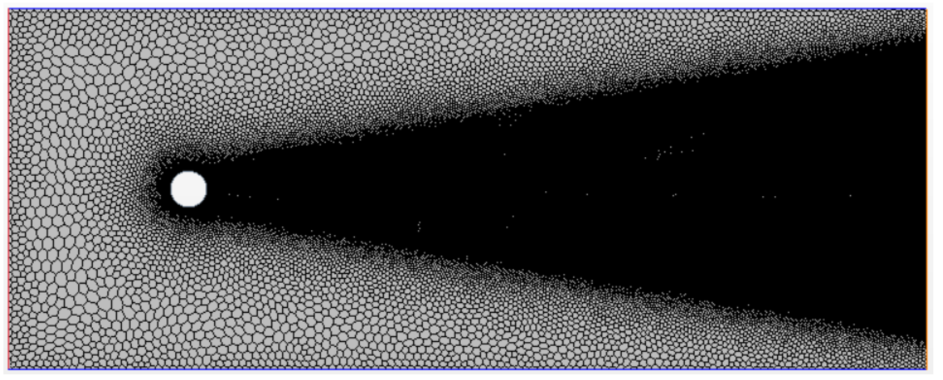
The design and construction of a high-quality grid is crucial to the success of CFD analysis, and these have the most direct influence on the precision of, convergence of, and time required to attain the solution. Within this domain, a mesh consisting of two-dimensional polyhedral cells was generated. Most of the cells were located around and downstream of the circular cylinder, in order to capture the vortexes in the wake behind this geometry. Additionally, a volumetric control was designed to refine the mesh around the body in order to keep the y+ value below 1, as illustrated in Figure 2.
The fluid was considered to be incompressible, turbulent, unsteady air. The density (ρ) of this selected fluid is equal to 1.18415 kg/m3 and its dynamic viscosity (µ) is equal to 1.85508 × 10⁻⁵ Pa·s. These values were assumed to be constant. The velocity at the inlet (u) ranged between 5 and 25 m/s, with an interval of 5 m/s between samples. Hence, a total of 5 different simulations were carried out. The Reynolds number of the conducted simulations ranged between 3200 and 16,000, depending on each case according to Equation (5):
R e = u · D ν ,
where u is the velocity of the fluid, D is the diameter of the circular cylinder and ν is the kinematic viscosity of the fluid.
Next, the CFD simulation data were interpolated into a 79 × 172 grid in order to fix the CNN input size.

2.2. CNN Architecture

A CNN is a type of non-linear universal approximator of a function, where the parameters of the non-linear approximator are known as synaptic weights. Thus, a CNN can be taken to be a non-linear regression. The quantity of input data is of utmost importance in order to obtain quality results.
The problem was analyzed using a time-based approach. In fact, in fluid dynamics, the state of a fluid at time t is significantly dependent on its state time, t-1. In other words, the focus is on the transition of the fluid between states. In regard to a neural network, this can be transposed to provide the network with the fluid’s state at time t-1 as an input.
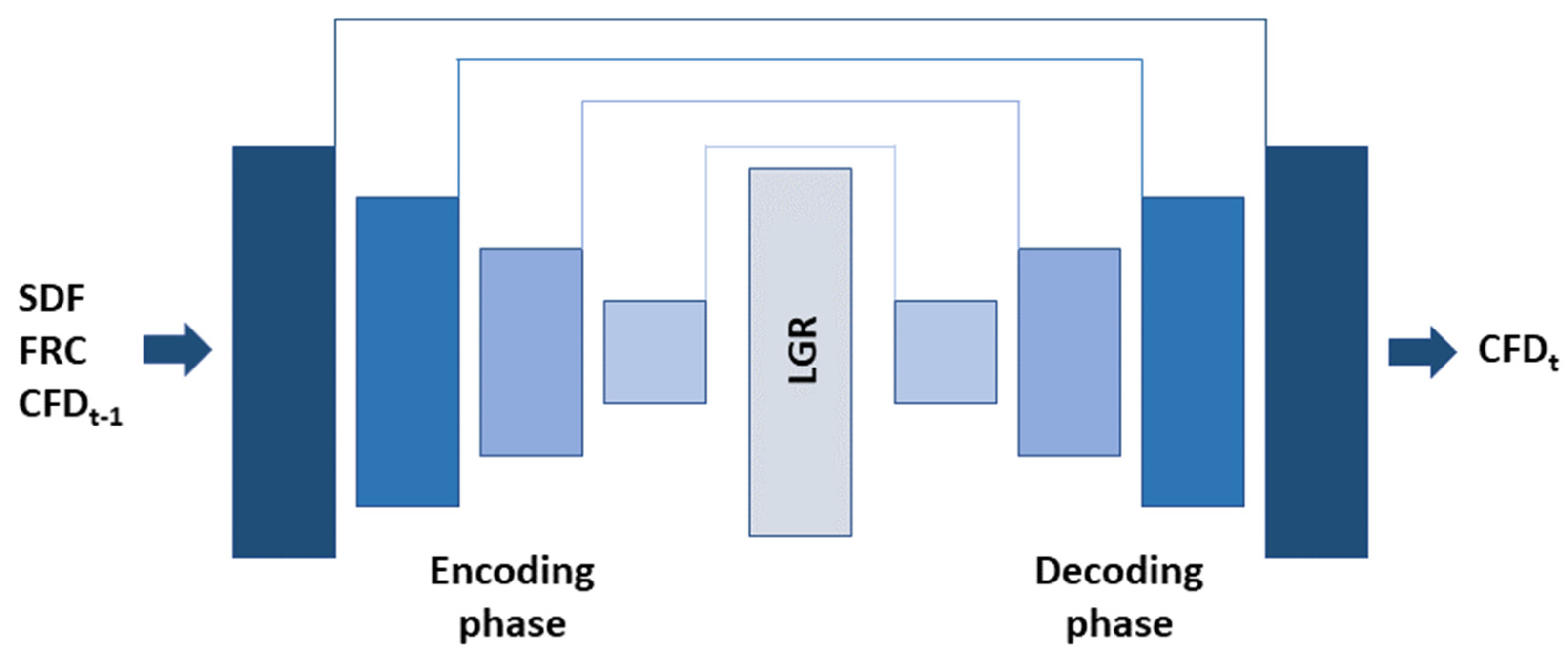
A U-Net architecture proposed by Ronneberger et al. [31] was employed. Initially, this network structure was employed for the segmentation of biomedical images. Since then, studies such as that by Thuerey et al. [17] have demonstrated the flexibility of this architecture to be adapted to the application of CFD to turbulent flow analysis. A U-Net network is a particular type of encoder–decoder network. This network consists of a series of convolutional layers which reduce the input data into a latent geometry representation (LGR), which is a representation of the basic features of the initial inputs of the CNN that enables the CNN to predict the patterns of interest easily and rapidly. Next, the LGR was extended using transposed convolution layers in order to map the streamwise and vertical velocities and the pressure fields. Figure 3 shows a simplified diagram of the network architecture.
Four encoder blocks constituted the encoding part, and 3 convolutional layers, with a kernel size of 5, made up each encoding block. After each convolution, a rectifier linear unit (ReLU) activation function was added, and after the last convolution layer of each block, a max pooling layer was included. Each block utilized a different number of filters, equal to 8, 16, 32 and 32 from the outermost to the innermost. The decoder carried out the reverse process of the encoder, using deconvolution layers to acquire one of the three variables being studied. The number of filters in the first deconvolution of each decoder block was multiplied by two. A detailed view of the architecture of the U-Net is provided in Figure 4. Python 3.9.6 [32] software was used to train and test the network.

2.3. Training Parameters

AdamW was selected as the optimizer for training the network. This algorithm is based on an adaptative moment estimation (Adam), which updates the gradient vector and the squared gradient using an exponential moving average. The coefficients β1 and β2 are the forgetting factors for the gradients and second moments of the gradients, respectively, and their values were both set to 0.5 [33].
AdamW is an updated version of the Adam optimizer, which improves regularization by decoupling the weight decay from the gradient-based update [34]. For this work, a L1-norm was employed as the loss function, the learning rate was set at 0.001, the weight decay at 0.005, the batch size at 64, and the data was split with a ratio of 0.7 for training and 0.3 for testing the model.

2.4. CNN Inputs

In this network, three different input layers were considered. The first pair were a flow region channel (FRC) and a signed distance function (SDF), which refer to the geometry shape and the features of the fluid throughout the different locations of the mesh, respectively. The latter represents the former instant of the field which is being analyzed.
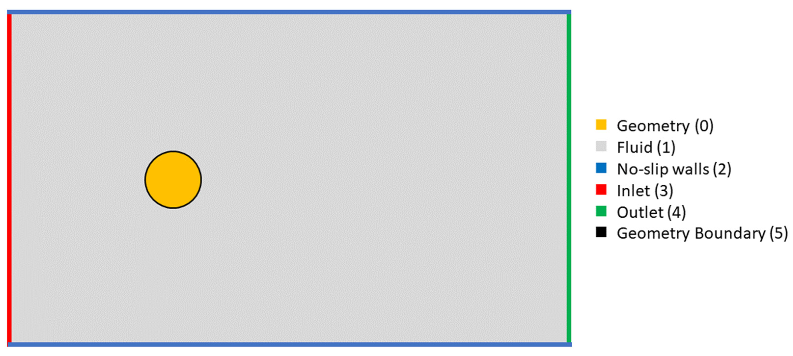
The FRC input layer was a multi-class channel containing information about the boundary conditions of the domain. The information was organized into 4 categories: 0 for the geometry, 1 for the free flow region, 2 for the slip conditions, 3 for the inlet and 4 for the outlet. Thus, no-slip conditions were employed in the top/bottom walls. Figure 5 displays a schematic view of the FRC layer.
SDF is a mathematical function that measures the relative distance between any point in the grid and the nearest boundary point of a closed geometry shape. [7]. The mathematical expression of this function is given by Equation (6):
S D F x = d x ,   ϑ Ω   i f   x Ω   d x ,   ϑ Ω   i f   x Ω c ,
where Ω is a subset of a metric space, X, with metric, d; and ϑΩ is the boundary of Ω. For any x   X:
d x ,   ϑ Ω : = inf y ϑ Ω d x , y ,
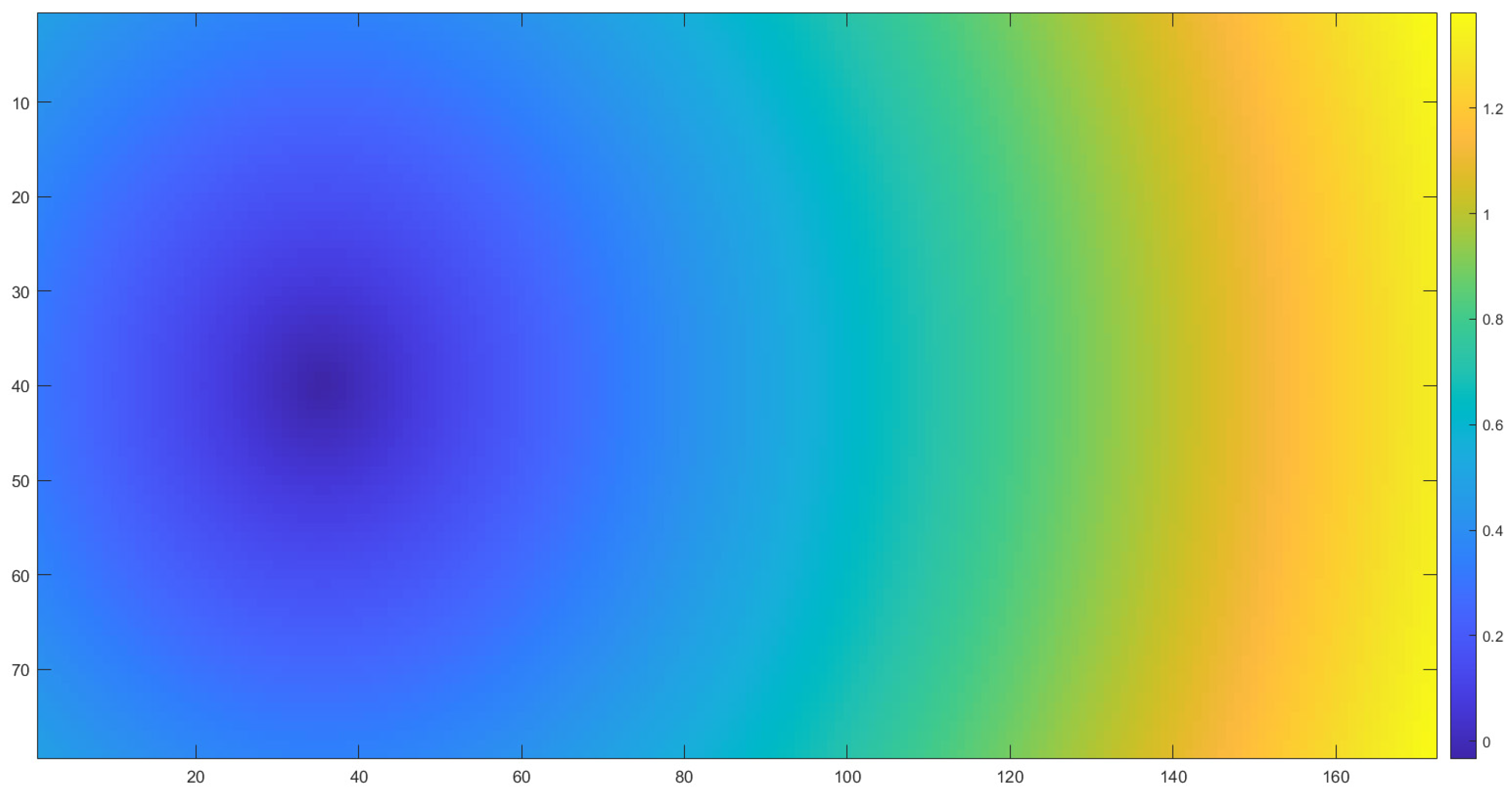
where inf denotes the infimum. Grid positions inside the interior of the obstacle (Ωc) are assigned negative distances [8]. Figure 6 shows the SDF that was generated for this work using a MATLAB [35] code, which allowed selection of the position and size of the geometry, as well as the size of the grid.
During the training of the CNN, the ground-truth CFD results were utilized as the third input to the CNN. In this case, the previous instant of the current CFD-analyzed sample was introduced as the third input. This allowed the CNN to learn the time patterns within the CFD results, and provided the time dependency on the previous state to the network. For the testing of the CNN, the result predicted in the previous instant was used as the current reference for the new prediction.

3. Results

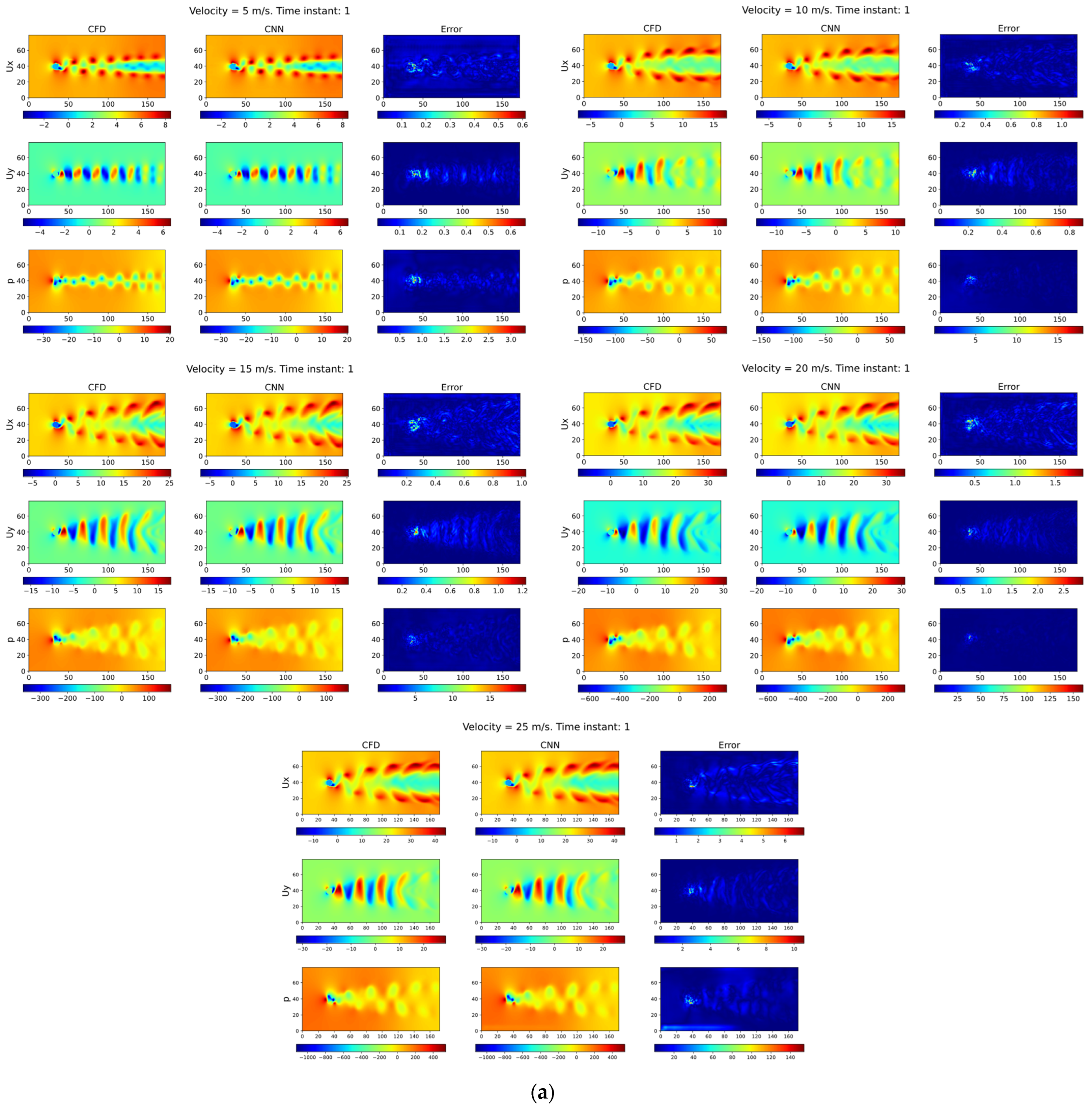
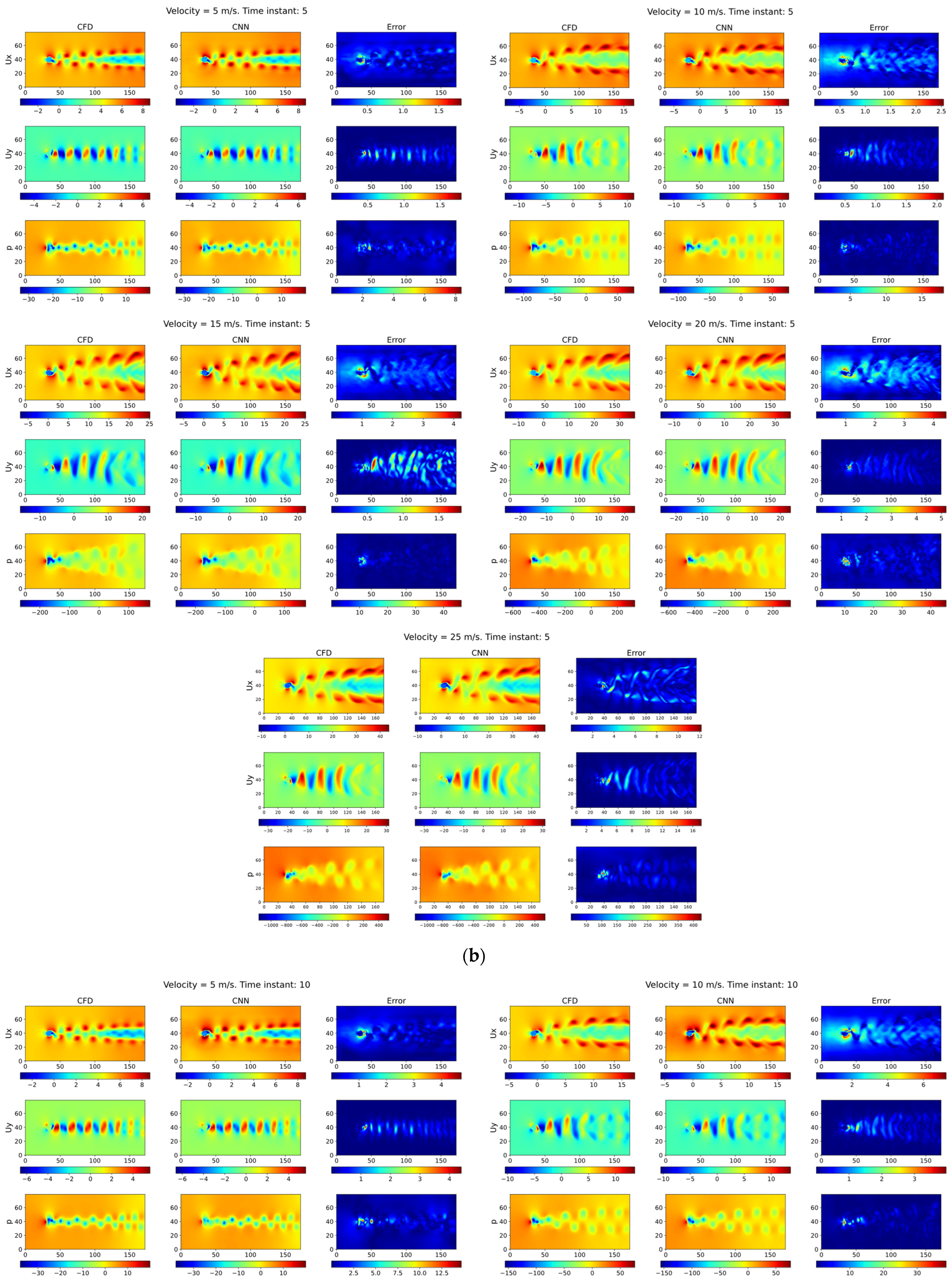
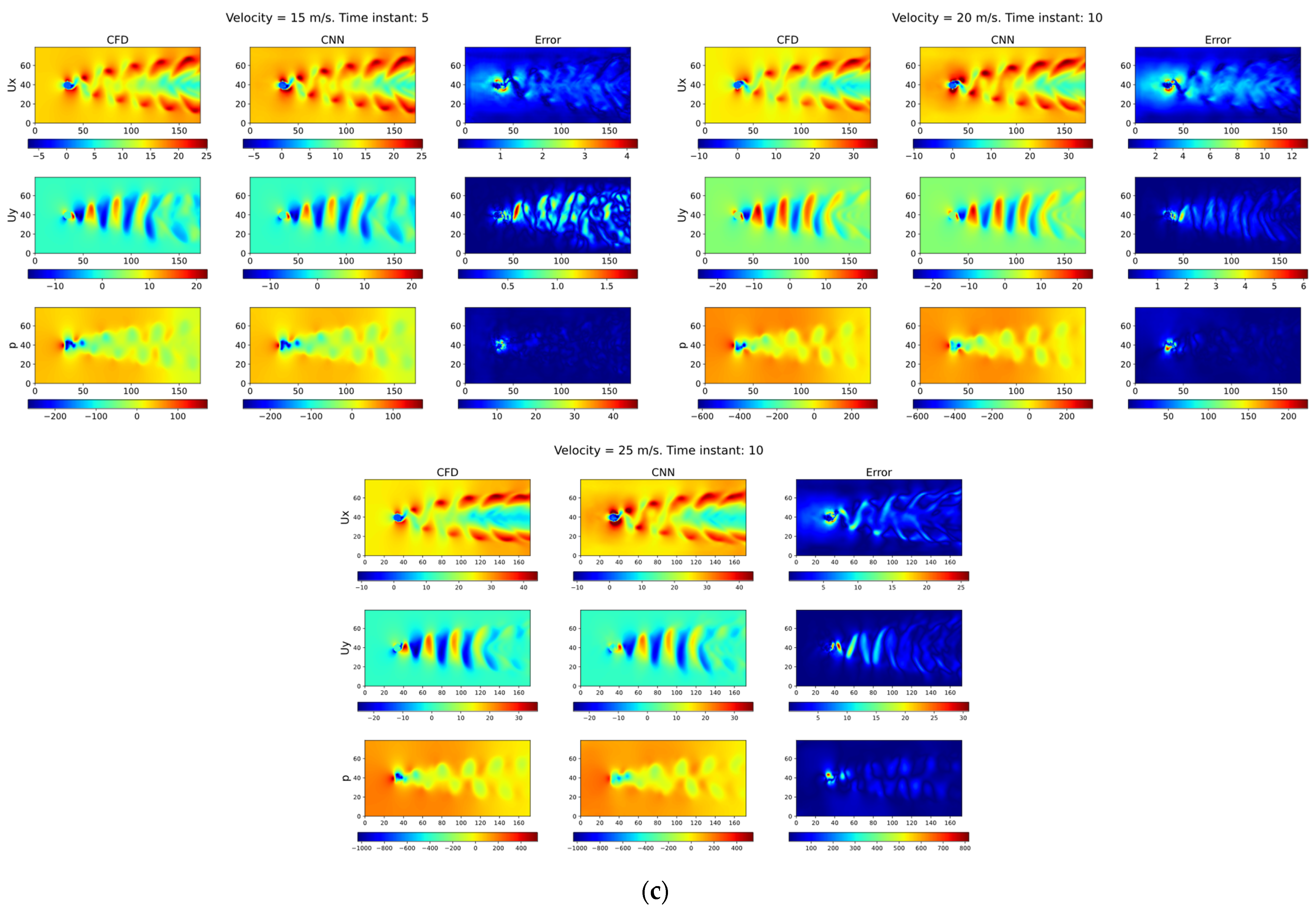
The neural network was trained three times, once for each of the variables studied. As aforementioned, the training was carried out using 70 % of the samples, and the number of epochs was set to 1000. Then, in the testing part of the study, the network was used to predict ten time instants for each of the five inlet velocities studied, for each of the three variables. During testing, the t-1 time instant was selected from the result of the previously iterated prediction, and the current prediction was compared with the corresponding ground-truth CFD sample, obtaining the absolute and relative errors. Figure 7 shows the CFD sample, the CNN prediction and the absolute error of the instants 1, 5 and 10, with respect to a random initial sample of the test set being used to determine the streamwise and vertical velocities and the pressure. In this figure, three samples are shown for every inlet velocity studied. Logically, the error incrementally increases with each of the new iterations, due to being based on the previous predictions. For higher inlet velocities, the changes between two adjacent samples were greater, which hindered the CNN predictions, resulting in larger error rates. Comparing the three variables studied, the predictions for pressure were of better precision than those obtained for both velocities, although the model still performed adequately for the velocity variables.
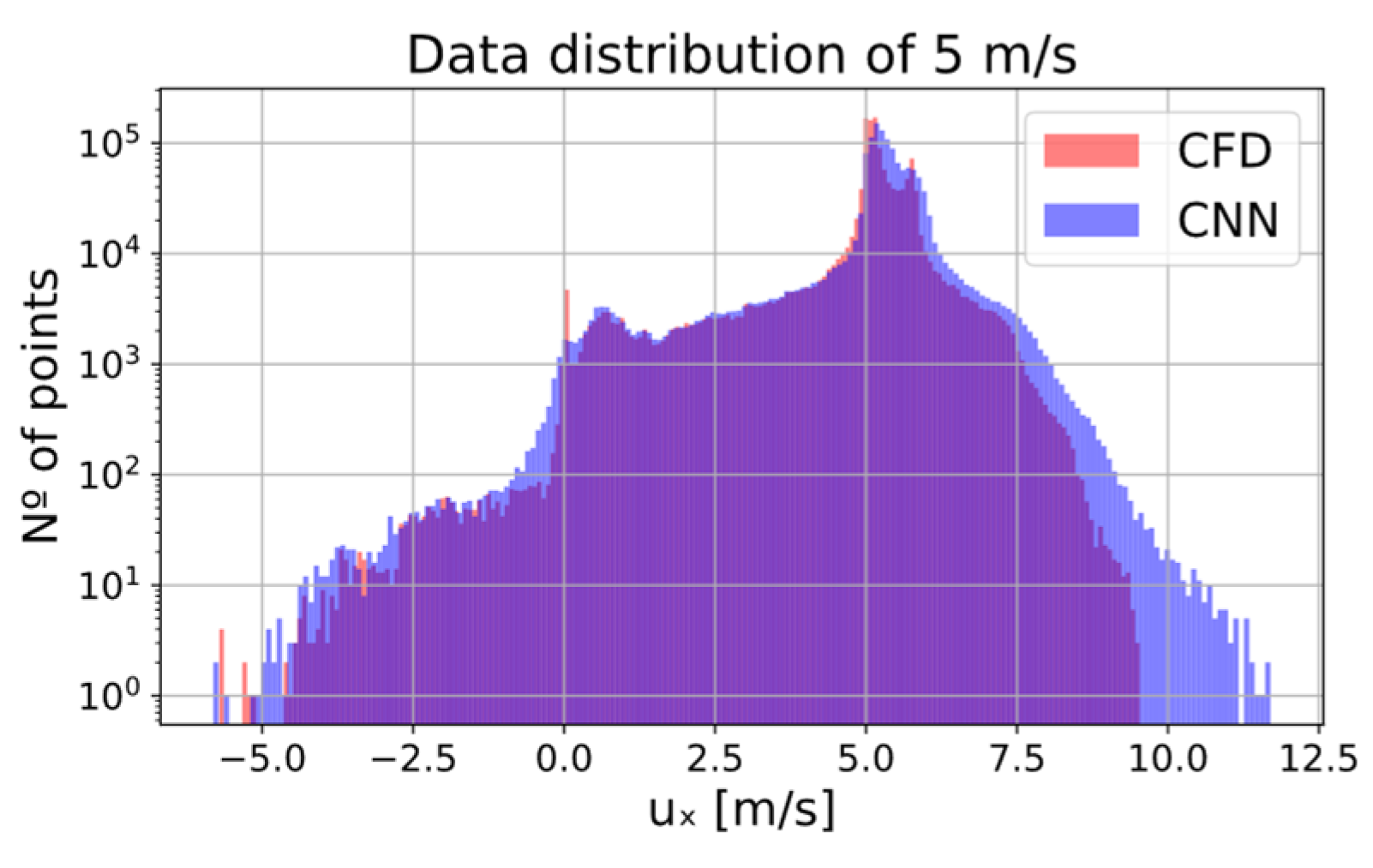
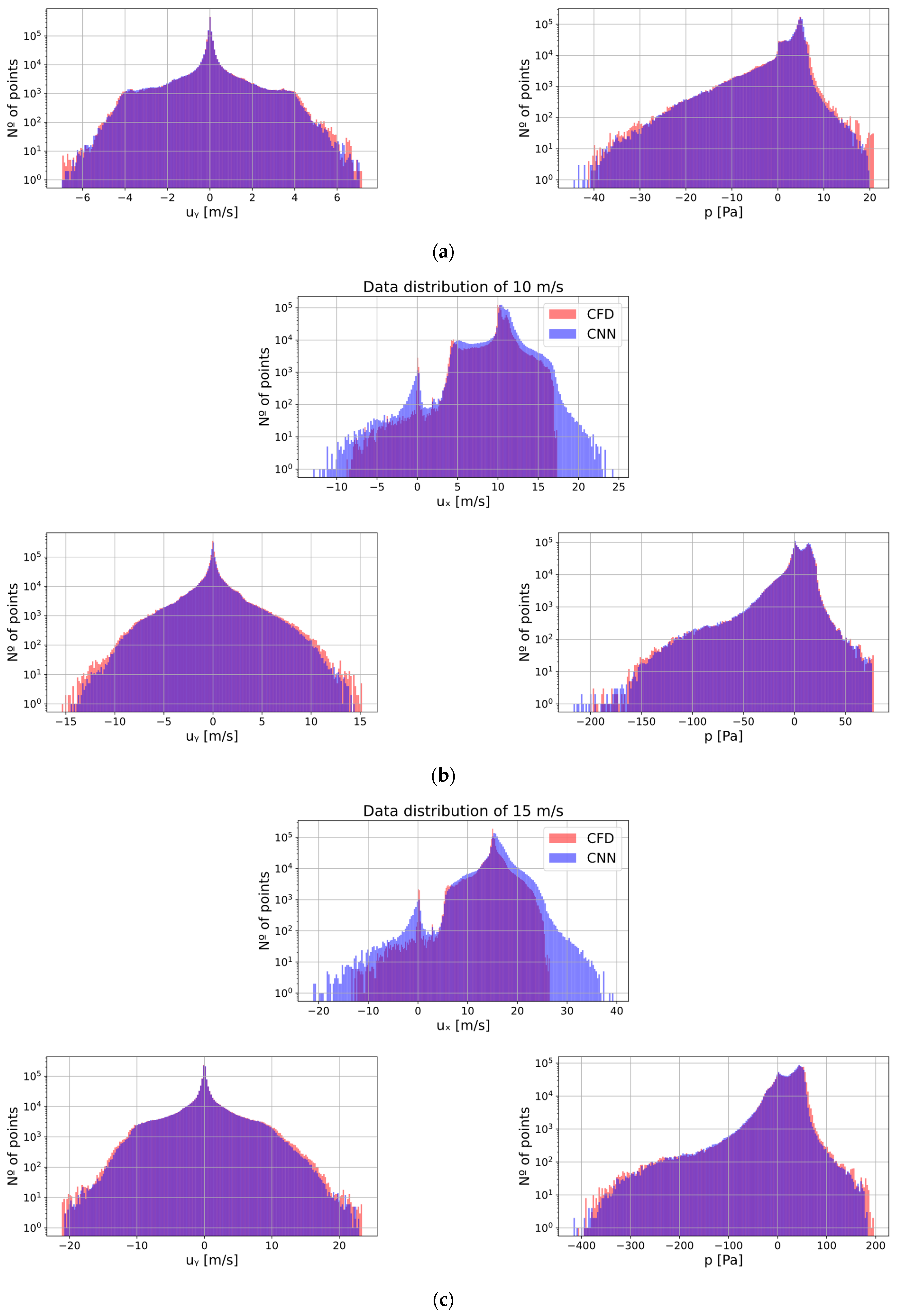
The histograms in Figure 8 show at which level the predictions fit with the ground-truth CFD data. In the cases of pressure and vertical velocity, the predicted values were very similar to those obtained in the CFD samples, except for the 25 m/s inlet velocity case, where the CNN outputted a group of excessively high negative values for the vertical velocity. In some testing cases, when a group of high value points with significant errors appeared, especially around or downstream from the circular cylinder, the error was transferred to the following predictions, which produced the data deviations observed in the histogram. For the streamwise velocity, this phenomenon also occurred, but to a lesser effect. The arithmetic mean and the variance for each of the inlet velocities is shown in Table 1, Table 2, Table 3, Table 4 and Table 5. The same conclusion extracted from the analysis of the histograms can be applied to the evaluation of the arithmetic mean and variance values obtained for the ground-truth CFD data and the CNN predictions. Here, shown in Table 5, the deviation produced in the vertical velocity was also appreciable. The arithmetic mean values obtained from the CNN predictions were, for every inlet velocity, higher than those obtained from the ground-truth CFD data. This occurred due to the aforementioned deviation phenomenon. One of the main objectives of the use of DL in CFD simulations is to reduce computational time. The duration of the training was 6.5, 6.2 and 6.3 h for the streamwise and vertical velocities and the pressure, respectively, giving a total of 19 h for the training phase. In the testing phase, calculating a prediction for 10 samples of any of the three variables studied took 0.49 s. Both training and testing were carried out using a NVIDIA Quadro RTX 6000 GPU. An Intel Xeon Gold 5120 CPU was used for the CFD simulations, which took a total of 15 h.

4. Conclusions

In the current work, a CNN with a U-Net structure was developed for the prediction of the streamwise and vertical velocities and the pressure fields downstream of a circular cylinder. Henceforth, a total of five different CFD-based unsteady simulations were carried out with the Reynolds number varying between 3200 and 16,000. The predictions were accomplished using a time-based approach, predicting the immediate future sample based on its dependency on its own previous state. The CNN was able to predict ten successive streamwise and vertical velocities and pressure fields using a sole architecture, with reasonably low error rates, particularly for the pressure. The error rate continuously increased throughout the new sample iterations, due to these being based on their previous prediction; and for larger inlet velocities, the error was higher. However, the approximation obtained is precise enough to compensate for the huge computational costs of CFD simulations. For future work, our CNN could be adapted to simulate and predict the fluid dynamics behavior of more aerodynamic geometries, such as airfoils or wings. Furthermore, the DL techniques could be applied to predict the best shape for an airfoil with an added gurney flap, in order to attain aerodynamic optimization.

Author Contributions

Conceptualization, A.A.-A. and E.Z.; methodology, A.A.-A.; software, U.F.-G. and E.Z.; validation, E.Z. and U.F.-G.; formal analysis, K.P.-P., E.Z. and A.T.-F.-B.; investigation, K.P.-P. and A.T.-F.-B.; resources, U.F.-G.; writing—original draft preparation, A.A.-A. and E.Z.; writing—review and editing, U.F.-G. All authors have read and agreed to the published version of the manuscript.

Funding

The current study was sponsored by the Government of the Basque Country-ELKARTEK21/10 KK-2021/00014 and IT1514-22 research program.

Institutional Review Board Statement

Not applicable.

Informed Consent Statement

Not applicable.

Data Availability Statement

All data presented in the current study are available upon reasonable request to the corresponding author.

Acknowledgments

The authors are grateful for the support provided by SGIker of UPV/EHU.

Conflicts of Interest

The authors declare no conflict of interest.

Nomenclature

NomenclatureDefinition
CFDComputational Fluid Dynamics
DLDeep Learning
CNNConvolutional Neural Network
DNNDeep Neural Network
RANSReynolds-Averaged Navier–Stokes
GANGenerative Adversarial Network
RNNRecurrent Neural Network
LGRLatent Geometry Representation
ReLURectifier Linear Unit
AdamAdaptative Moment Estimation
SDFSigned Distance Function
FRCFlow Region Channel
β1Forgetting factor for gradients
β2Forgetting factor for second moment gradients
DDiameter of the circle
FBody forces
KMultiplying constant for the loss functions
LtLoss function
Ρ Pressure
p Fluid density
ReReynolds number
u x Streamwise velocity
u y Vertical velocity
u Inlet velocity to the domain

References

  1. Anderson, J.D., Jr. Basic Philosophy of CFD. In Computational Fluids Dynamics; Springer: Rhode-Saint-Genèse, Belgium, 2009; pp. 3–15. [Google Scholar]
  2. Tao, J.; Sun, G. Application of deep learning based multi-fidelity surrogate model to robust aerodynamic design optimization. Aerosp. Sci. Technol. 2019, 92, 722–737. [Google Scholar] [CrossRef]
  3. Zhang, X.; Xie, F.; Ji, T.; Zhu, Z.; Zheng, Y. Multi-Fidelity Deep Neural Network Surrogate Model for Aerodynamic Shape Optimization. Comput. Methods Appl. Mech. Eng. 2021, 373, 113485. [Google Scholar] [CrossRef]
  4. Yan, X.; Zhu, J.; Kuang, M.; Wang, X. Aerodynamic Shape Optimization Using a Novel Optimizer Based on Machine Learning Techniques. Aerosp. Sci. Technol. 2019, 86, 826–835. [Google Scholar] [CrossRef]
  5. Hanna, B.N.; Dinh, N.T.; Youngblood, R.W.; Bolotnov, I.A. Coarse-Grid Computational Fluid Dynamic (CG-CFD) Error Prediction Using Machine Learning. arXiv 2017, arXiv:1710.09105. [Google Scholar]
  6. Bao, H.; Feng, J.; Dinh, N.; Zhang, H. Computationally efficient CFD prediction of bubbly flow using physics-guided deep learning. Int. J. Multiph. Flow 2020, 131, 103378. [Google Scholar] [CrossRef]
  7. Guo, X.; Li, W.; Iorio, F. Convolutional Neural Networks for Steady Flow Approximation. In Proceedings of the 22nd ACM SIGKDD International Conference on Knowledge Discovery and Data Mining, San Francisco, CA, USA, 13–17 August 2016; Association for Computing Machinery: New York, NY, USA, 2016; pp. 481–490. [Google Scholar]
  8. Ribeiro, M.D.; Rehman, A.; Ahmed, S.; Dengel, A. DeepCFD: Efficient Steady-State Laminar Flow Approximation with Deep Convolutional Neural Networks. arXiv 2020, arXiv:2004.08826. [Google Scholar]
  9. Kashefi, A.; Rempe, D.; Guibas, L.J. A point-cloud deep learning framework for prediction of fluid flow fields on irregular geometries. Phys. Fluids 2021, 33, 027104. [Google Scholar] [CrossRef]
  10. Ling, J.; Kurzawski, A.; Templeton, J. Reynolds averaged turbulence modelling using deep neural networks with embedded invariance. J. Fluid Mech. 2016, 807, 155–166. [Google Scholar] [CrossRef]
  11. Lee, S.; You, D. Prediction of Laminar Vortex Shedding over a Cylinder Using Deep Learning. arXiv 2017, arXiv:1712.07854. [Google Scholar]
  12. Liu, Y.; Lu, Y.; Wang, Y.; Sun, D.; Deng, L.; Wang, F.; Lei, Y. A CNN-based shock detection method in flow visualization. Comput. Fluids 2019, 184, 1–9. [Google Scholar] [CrossRef]
  13. Deng, L.; Wang, Y.; Liu, Y.; Wang, F.; Li, S.; Liu, J. A CNN-based vortex identification method. J. Vis. 2019, 22, 65–78. [Google Scholar] [CrossRef]
  14. Nowruzi, H.; Ghassemi, H.; Ghiasi, M. Performance predicting of 2D and 3D submerged hydrofoils using CFD and ANNs. J. Mar. Sci. Technol. 2017, 22, 710–733. [Google Scholar] [CrossRef]
  15. Mohan, A.; Daniel, D.; Chertkov, M.; Livescu, D. Compressed Convolutional LSTM: An Efficient Deep Learning Framework to Model High Fidelity 3D Turbulence. arXiv 2019, arXiv:1903.00033. [Google Scholar]
  16. Fang, R.; Sondak, D.; Protopapas, P.; Succi, S. Deep Learning for Turbulent Channel Flow. arXiv 2018, arXiv:1812.02241. [Google Scholar]
  17. Thuerey, N.; Weißenow, K.; Prantl, L.; Hu, X. Deep Learning Methods for Reynolds-Averaged Navier–Stokes Simulations of Airfoil Flows. AIAA J. 2020, 58, 25–36. [Google Scholar] [CrossRef]
  18. Abucide-Armas, A.; Portal-Porras, K.; Fernandez-Gamiz, U.; Zulueta, E.; Teso-Fz-Betoño, A. A Data Augmentation-Based Technique for Deep Learning Applied to CFD Simulations. Mathematics 2021, 9, 1843. [Google Scholar] [CrossRef]
  19. Portal-Porras, K.; Fernandez-Gamiz, U.; Ugarte-Anero, A.; Zulueta, E.; Zulueta, A. Alternative Artificial Neural Network Structures for Turbulent Flow Velocity Field Prediction. Mathematics 2021, 9, 1939. [Google Scholar] [CrossRef]
  20. Agostini, L. Exploration and prediction of fluid dynamical systems using auto-encoder technology. Phys. Fluids 2020, 32, 067103. [Google Scholar] [CrossRef]
  21. King, R.; Hennigh, O.; Mohan, A.; Chertkov, M. From Deep to Physics-Informed Learning of Turbulence: Diagnostics. arXiv 2018, arXiv:1810.07785. [Google Scholar]
  22. Gonzalez, F.J.; Balajewicz, M. Deep Convolutional Recurrent Autoencoders for Learning Low-Dimensional Feature Dynamics of Fluid Systems. arXiv 2018, arXiv:1808.01346. [Google Scholar]
  23. Maulik, R.; Lusch, B.; Balaprakash, P. Reduced-Order Modeling of Advection-Dominated Systems with Recurrent Neural Networks and Convolutional Autoencoders. Phys. Fluids 2021, 33, 037106. [Google Scholar] [CrossRef]
  24. Iaccarino, G.; Ooi, A.; Durbin, P.; Behnia, M. Reynolds averaged simulation of unsteady separated flow. Int. J. Heat Fluid Flow 2003, 24, 147–156. [Google Scholar] [CrossRef]
  25. Siemens Software. Available online: https://www.plm.automation.siemens.com/global/en/ (accessed on 20 November 2022).
  26. Osher, S.; Chakravarthy, S. Upwind schemes and boundary conditions with applications to Euler equations in general geometries. J. Comput. Phys. 1983, 50, 447–481. [Google Scholar] [CrossRef]
  27. Menter, F.R. Two-equation eddy-viscosity turbulence models for engineering applications. AIAA J. 1994, 32, 1598–1605. [Google Scholar] [CrossRef] [Green Version]
  28. Rajani, B.; Kandasamy, A.; Majumdar, S. Numerical simulation of laminar flow past a circular cylinder. Appl. Math. Model. 2009, 33, 1228–1247. [Google Scholar] [CrossRef]
  29. Rahman, M.; Karim, M.; Alim, A. Numerical investigation of unsteady flow past a circular cylinder using 2-D finite volume method. J. Nav. Arch. Mar. Eng. 1970, 4, 27–42. [Google Scholar] [CrossRef] [Green Version]
  30. Aramendia, I.; Fernandez-Gamiz, U.; Guerrero, E.Z.; Lopez-Guede, J.M.; Sancho, J. Power Control Optimization of an Underwater Piezoelectric Energy Harvester. Appl. Sci. 2018, 8, 389. [Google Scholar] [CrossRef]
  31. Ronneberger, O.; Fischer, P.; Brox, T. U-Net: Convolutional Networks for Biomedical Image Segmentation. In Medical Image Computing and Computer-Assisted Intervention—MICCAI 2015; Navab, N., Hornegger, J., Wells, W.M., Frangi, A.F., Eds.; Lecture Notes in Computer Science; Springer International Publishing: Cham, Switzerland, 2015; Volume 9351, pp. 234–241. [Google Scholar]
  32. Welcome to Python.Org. Available online: https://www.python.org/ (accessed on 20 November 2022).
  33. Kingma, D.P.; Ba, J. Adam: A Method for Stochastic Optimization. arXiv 2014, arXiv:1412.6980. [Google Scholar]
  34. Loshchilov, I.; Hutter, F. Decoupled Weight Decay Regularization. In Proceedings of the International Conference on Learning Representations, New Orleans, LA, USA, 6–9 May 2019. [Google Scholar]
  35. MATLAB. MathWorks. Available online: https://www.mathworks.com/products/matlab.html (accessed on 20 November 2022).
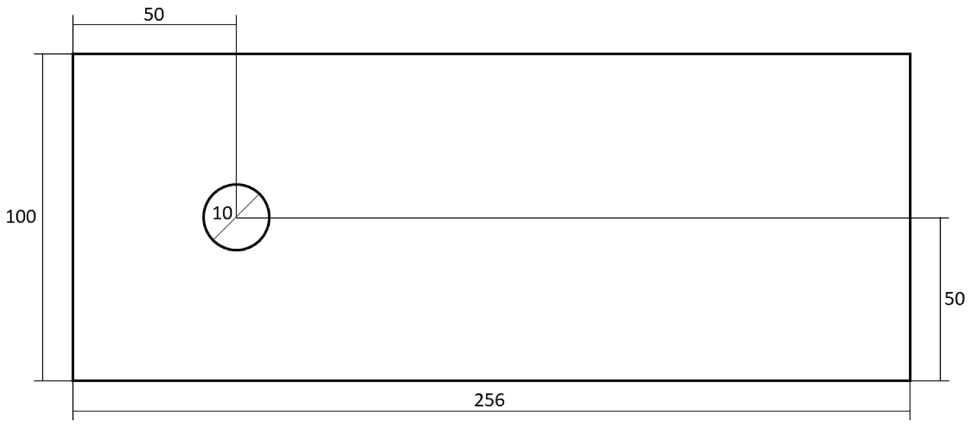
Figure 1. Computational domain (not to scale).
Jmse 11 00239 g001
Figure 2. Mesh distribution around the cylinder.
Jmse 11 00239 g002
Figure 3. U-Net with 3 decoders.
Jmse 11 00239 g003
Figure 4. Architecture of the CNN.
Jmse 11 00239 g004
Figure 5. Diagram of the multi-class labelling of flow regions (not to scale).
Jmse 11 00239 g005
Figure 6. SDF of a circle.
Jmse 11 00239 g006
Figure 7. Results of the predictions obtained using the CNN for 5, 10, 15, 20 and 25 m/s at (a) the first time instant, (b) the fifth time instant and (c) the tenth time instant.
Jmse 11 00239 g007aJmse 11 00239 g007bJmse 11 00239 g007c
Figure 8. Data distribution of ux, uy and p for inlet velocities of (a) 5 m/s, (b) 10 m/s, (c) 15 m/s, (d) 20 m/s and (e) 25 m/s.
Jmse 11 00239 g008aJmse 11 00239 g008bJmse 11 00239 g008c
Table 1. Comparison of arithmetic mean and variance between the ground-truth CFD data and the CNN predictions for the streamwise velocity of 5 m/s.
5 m/sCFDCNN
uxuypuxuyp
Arithmetic mean (µ)4.99560.00490.39905.1363−0.00792.8473
Variance1.34780.961518.57831.54020.897015.7479
Table 2. Comparison of arithmetic mean and variance between the ground-truth CFD data and the CNN predictions for the streamwise velocity of 10 m/s.
10 m/sCFDCNN
uxuypuxuyp
Arithmetic mean (µ)9.9913−0.00794.328010.3442−0.02474.4879
Variance5.30173.4790209.16355.30773.1156193.8350
Table 3. Comparison of arithmetic mean and variance between the ground-truth CFD data and the CNN predictions for the streamwise velocity of 15 m/s.
15 m/sCFDCNN
uxuypuxuyp
Arithmetic mean (µ)14.99480.016821.819015.7475−0.017320.1163
Variance9.064712.97191129.471310.500811.4202962.2498
Table 4. Comparison of arithmetic mean and variance between the ground-truth CFD data and the CNN predictions for the streamwise velocity of 20 m/s.
20 m/sCFDCNN
uxuypuxuyp
Arithmetic mean (µ)19.98890.053946.739620.87350.017843.9651
Variance21.651322.13454063.954923.243619.61423615.1444
Table 5. Comparison of arithmetic mean and variance between the ground-truth CFD data and the CNN predictions for the streamwise velocity of 25 m/s.
25 m/sCFDCNN
uxuypuxuyp
Arithmetic mean (µ)24.98080.032972.160125.4197−0.194668.5239
Variance40.707033.765111124.312637.9972129.34318799.3459
Disclaimer/Publisher’s Note: The statements, opinions and data contained in all publications are solely those of the individual author(s) and contributor(s) and not of MDPI and/or the editor(s). MDPI and/or the editor(s) disclaim responsibility for any injury to people or property resulting from any ideas, methods, instructions or products referred to in the content.