A Tidal Flat Adjacent to a Fringe Mangrove Forest Mitigates pCO₂ Increases and Enhances Lateral Export of Dissolved Carbon

Abstract

Carbon export from mangrove forests to the oceans partly acts as a sink for atmospheric CO₂, exceeding the rate of carbon burial in mangrove soils. Primary production in ecosystems adjacent to mangroves may prevent degassing and enhance further carbon export from mangroves to the oceans. In this study, we continuously monitored carbonate chemistry parameters (pCO₂, dissolved inorganic carbon (DIC), total alkalinity (TA)) and dissolved organic carbon (DOC) in a tidal flat adjacent to a fringe mangrove forest over a spring-neap tidal cycle. Mean pCO₂ during the entire period was 923 ± 318 μatm, and the export of TA, DIC, and DOC from the mangroves to the ocean was 36 ± 26 mmol m⁻² d⁻¹, 42 ± 39 mmol m⁻² d⁻¹, and 10 ± 9 mmol m⁻² d⁻¹, respectively. Semi-monthly pCO₂ variations in the mangrove front were controlled by the tidal level during spring tide and by photosynthesis and respiration on the tidal flat during neap tide. This means that during neap tide, photosynthesis on the tidal flat offset the increase in pCO₂ caused by the porewater export from the mangrove soil. The DIC/TA export ratio in this study was 1.17 ± 0.08, which was lower than the global average of 1.41 ± 1.39, indicating that the tidal flat adjacent to the mangrove forest may act as a buffer zone to mitigate the increase in pCO₂, resulting in much of the exported DIC being stored in the ocean.

1. Introduction

Coastal vegetation such as mangroves, salt marshes, and seagrasses are known as blue carbon ecosystems and absorb atmospheric CO₂ and store organic carbon in sediments [1]. These ecosystems are estimated to sequester carbon at a rate of approximately 31.2–82.8 Tg C yr⁻¹, with carbon sequestration within the soil on a scale of 100 to 1000 years [2]. Although blue carbon ecosystems account for only 0.2% of the ocean’s surface area, they are responsible for sequestering carbon which is equivalent to about 50% of the carbon buried in ocean sediments each year [2,3,4].

A portion of the organic carbon buried in mangrove soils decomposes into dissolved inorganic carbon (DIC), which is subsequently outwelled into the adjacent waters through tidal pumping [5,6]. This outwelling causes an increase in the partial pressure of carbon dioxide (pCO₂) in the mangrove adjacent waters [7,8,9,10]. The export of carbon from mangroves into the oceans plays a pivotal role within the intricate network of carbon cycling that facilitates the sequestration of atmospheric CO₂ [11,12]. While the waters adjacent to mangroves release a large amount of CO₂ into the atmosphere, the lateral export of total alkalinity (TA) and DIC from mangrove ecosystems to the ocean serves as a prominent carbon sink [11]. This process accounts for approximately 63% of the greenhouse gases absorbed by these mangrove ecosystems, exceeding the carbon stored in the soil [11]. Furthermore, under conditions where TA is abundantly supplied to the ocean, it may enhance the atmospheric CO₂ uptake into the ocean [13,14]. The export of dissolved organic carbon (DOC) from blue carbon ecosystems into the ocean has also garnered considerable attention, representing a novel reservoir for carbon sequestration [15]. In particular, organic matter originating from mangroves is poised to persist in the ocean for an extended duration as refractory organic matter [16]. On a global scale, the lateral exports of mangrove-derived DIC and DOC emerge as a consequential carbon sink that imparts approximately 29–48% of global river inflows into the ocean [11,17]. Nevertheless, the necessity for further data accumulation persists, given the observed variability in the reported values about the lateral export of TA, DIC, and DOC into the ocean [18].

In comparison to aquatic ecosystems such as seagrass meadows, tidal flats, salt marshes and wetlands, mangrove adjacent waters show characteristic patterns of variation in dissolved oxygen (DO) and carbonate chemistry parameters (pCO₂, DIC, TA). In the aquatic ecosystems, DO has a daytime maximum and a nighttime minimum due to photosynthesis and respiration by abundant organisms [19,20,21]. In contrast, in mangrove adjacent waters, DO and carbonate chemistry parameters vary in response to tidal levels [22,23,24,25]. Hence, the dynamics of carbonate chemistry parameters in mangrove adjacent waters vary greatly depending on the semi–monthly tidal cycle, from spring to neap tides [6,9,10,23]. However, the variability of pCO₂ in the combined environment of mangrove forests and these aquatic ecosystems has rarely been studied [26]. The carbon cycle, including mangroves and adjacent ecosystems, will provide further insight into the ability of mangroves to store carbon in the ocean.

Fringe mangrove forests, which form parallel to the coastline, are directly exposed to tides and waves and tend to receive little sediment supply from the land [27]. As a result, the area of mangroves is smaller and soil carbon accumulation is lower than in riverine mangrove forests where alluvial sediment supply is abundant [27,28]. Therefore, the increase in pCO₂ due to tidal pumping would be less in fringe mangroves than in riverine mangroves because of the lower organic carbon accumulation. However, there is a notable lack of research on the outwelling process and CO₂ dynamics in the adjacent water specifically in fringe mangroves.

The primary objectives of this investigation are as follows: (1) to elucidate the controlling factors that cause variations in pCO₂ between spring and neap tides in a tidal flat adjacent to a fringe mangrove forest and to quantify the CO₂ efflux from the water to the atmosphere, and (2) to assess the lateral export of TA, DIC, and DOC to the ocean from the mangrove ecosystems located at the northern limit of mangrove distribution in the Indo-Pacific region. In line with these objectives, we conducted continuous observations of carbonate chemistry parameters and DOC over a spring-neap tidal cycle on a tidal flat formed in front of a fringe mangrove forest on Iriomote Island, Okinawa, Japan.

2. Materials and Methods

2.1. Field Site

This study was carried out on the Yubu coast of Iriomote Island, Okinawa, Japan, located at the northern limit of mangrove distribution within the Indo-Pacific region (Figure 1). The Yubu coast serves as a typical example of a fringe mangrove forest, characterized by mangrove communities aligned parallel to the shoreline. The elevation of the mangrove edge along the shoreline was 28 cm above mean sea level [29]. During low tide, there is an approximately 1 km expanse of a tidal flat that separates the mangrove area from the adjacent ocean. The mangrove area, estimated using Google Earth’s polygon function, is 11.3 ha. The dominant mangrove species are Rhizophora stylosa and Bruguiera gymnorrhiza [30]. Along the Yubu coast, the mangroves exhibit a distinct zonation pattern, with different species occurring sequentially from the seaward side to the landward side, namely Sonneratia alba, R. stylosa, and B. gymnorrhiza, respectively (Figure 1). The maximum tree height of S. alba, R. stylosa, and B. gymnorrhiza are 5.7 m, 5.7 m, and 11.1 m, respectively [29]. Behind the mangrove forest lie agricultural fields.

The mangrove forest is inundated by high tides of up to approximately 1.1 m during spring tides, classifying it as a microtidal area. According to the Japan Meteorological Agency, the mean temperatures in summer and winter between the years 1991 and 2020 were 29.1 °C and 19.6 °C, respectively. The mean annual precipitation during the same period was 2095 mm, with a tendency to increase during the rainy season in June and the typhoon season in September and October.

2.2. Sample Collection and Fieldwork

Fieldwork was conducted from 4th to 13th July, 2023. Within this timeframe, a temporary platform was installed within a tidal pool on the tidal flat (blue star in Figure 1) for the continuous monitoring of environmental variables. A pCO₂ analyzer and floating water sensors were attached to the platform to collect surface water quality data. The surface pCO₂, water temperature, salinity, and DO were recorded at 10-min intervals. Surface air temperature was measured at 5-min intervals. Current velocity at 15 cm from the bottom and the water level were measured at 5-min intervals.

To determine the temporal alterations in carbon (DOC) and carbonate chemistry parameters (TA, DIC, and δ¹³C_DIC), water samples were collected in front of the mangrove forest at intervals of 2 h over a continuous 24-h period, encompassing both spring tide (4th to 5th July) and neap tide (11th to 12th July) (blue star in Figure 1). Simultaneously, samples of river water, subtidal water, and porewater originating from the mangrove forest and the tidal flat were retrieved to ascertain the properties of these distinct end-member waters (Figure 1). Subtidal water was collected during the flood tide on 4th July, while porewater was collected during the low tide on both 4th July and 11th July. Porewater was collected by digging a hole approximately 20 cm deep, removing the water once with a pump, and then collecting the eluted water. Water samples for TA and DIC were collected in 250-mL Duran bottles (SCHOTT AG, Mainz, Germany) and water samples for δ¹³C_DIC were collected in 10-mL glass vials with Teflon-lined screw caps. To prevent biological activity, water samples for TA, DIC, and δ¹³C_DIC were treated with a saturated solution of mercuric chloride (10 g HgCl₂ per 100 mL water). Water samples for DOC were collected in a 60 mL polypropylene container, which had been subject to acid pretreatment. To avoid degradation, water samples for DOC analysis were filtered through a 0.75 μm precombusted (450 °C, 3 h) filter (Whatman GF/F, Whatman GE Healthcare Life Sciences, England) and stored at −20 °C until analysis.

Ten soil cores were collected from each species-dominated sites down to the substrate using the Geoslicer NM5 (crosses in Figure 1) [31]. The Geoslicer NM5 is a soil core sampler that is capable of taking an undisturbed soil core sample with a cross-sectional area of 15 cm². One representative soil core was analyzed from the ten cores. A surface sediment sample from the tidal flat was also collected and analyzed. There was no precipitation during the survey.

2.3. Analytical Protocol

The pCO₂ was measured with non-dispersive infrared (NDIR) sensors (GMP343, VAISALA Corporation, Helsinki, Finland), which were coupled with desiccant (Drierite, Thermo Scientific Chemicals, Tokyo, Japan), and an equilibrator system that was furnished with a gas-permeable membrane (PolyTetraFluoroEthylene (PTFE) tube, Sumitomo Electric Fine Polymer, Inc., Osaka, Japan) [32]. Before conducting the field surveys, the analyzer was calibrated utilizing pure nitrogen (0 µatm CO₂) and a CO₂ span of 801 µatm (Taiyo Nippon Sanso Co., Ltd., Tokyo, Japan). The NDIR sensor exhibited an accuracy of ±10 μatm for 801 μatm of CO₂ gas at the end of each survey. Water temperature (accuracy ± 0.01 °C), salinity (accuracy ± 0.01), and DO (accuracy ± 1%) at the platform were measured using a RINKO-Profiler (ASTD102, JFE Advantech, Nishinomiya, Japan). Current velocity (accuracy ± 1 cm s⁻¹) was measured using a COMPACT-EM (JFE Advantech). Water level (accuracy ± 0.4 cm) and air temperature (accuracy ± 0.19 °C) were measured utilizing a HOBO U20L-04 (ONSET, Computer Corporation, Bourne, MA, USA). Wind speed data were obtained from the Iriomote station of the Japan Meteorological Agency (located approximately 16 km from the Yubu coast).

TA and DIC were determined using a batch-sample analyzer (ATT-05, Kimoto Electric Co., Ltd., Osaka, Japan) through the implementation of the Gran plot method [33]. The accuracies of TA and DIC were estimated to be ±1 µM and ±2 µM, respectively, utilizing the certified reference material (CRM Batch 196, Scripps Institution of Oceanography, UC San Diego, USA). δ¹³C_DIC was determined by the headspace equilibration method [34]. The headspace gas of the tube purged with pure helium was equilibrated overnight and then fed to Gasbench-IRMS (Thermo Fisher Scientific, DELTA V, Cleveland, OH, USA) using an autosampler to determine the δ¹³C of CO₂. Standard materials such as NBS19 (TS limestone) and LSVEC (Li carbonate) were used as international standards, while SPK was used as a working standard during calibration. The analytical error for δ¹³C_DIC was consistently within the range of 0.1‰. DOC was quantified through a process of high-temperature combustion oxidation employing the Shimadzu TOC-V Analyzer (Shimadzu Co. Ltd., Kyoto, Japan). The instrument’s accuracy was ensured through calibration involving a sequence of aqueous solutions containing potassium hydrogen phthalate, and it was thoroughly rinsed with Milli-Q water to minimize the coefficient of variation. The reproducibility of DOC measurements was considered < 2%.

The particle size of the surface sediments was determined using the pipette method, while the soil color was assessed by examining samples that had been dried at 110 °C for 24 h, following the guidelines provided by the Munsell soil color chart. Subsequently, the dried samples were subjected to a temperature of 550 °C for 3 h, allowing for the calculation of ignition loss based on the observed mass change. A portion of the dried samples was finely ground using a pestle and mortar, passed through a 0.5 mm mesh sieve, and treated with 1M HCl to remove inorganic carbon. Elemental composition analyses, specifically for soil organic carbon (SOC) and total nitrogen (TN), were then conducted in duplicate using an elemental analyzer (Flash EA 1112; Thermo Electron, Bremen, Germany) with a measurement involving 30–50 mg of dry sample.

2.4. Data Analysis

The water-air CO₂ flux (mol m⁻² h⁻¹) was calculated as follows:

$${\mathrm{C}\mathrm{O}}_2\mathrm{f}\mathrm{l}\mathrm{u}\mathrm{x}=k·K_0·{∆p\mathrm{C}\mathrm{O}}_2$$

(1)

where k is the gas transfer velocity (m h⁻¹), $K_0$ is the solubility coefficient of CO₂ (mol m⁻³ atm⁻¹), and ${∆p\mathrm{C}\mathrm{O}}_2$ is the difference in CO₂ fugacity (≅partial pressure) between water and atmosphere, respectively. A positive CO₂ flux indicates a CO₂ efflux from water to the atmosphere. The in-situ mole fraction of CO₂ was converted to the pCO₂ using an equation of state for the vapor phase, with the in-situ air pressure as 1 atm [35]. The value of atmospheric pCO₂ was given as 416 μatm (421 ppm), referring to the Yonaguni station of the Japan Meteorological Agency (located approximately 95 km from the Yubu coast). $K_0$ was determined using the Weiss equation [35], which is a function of salinity and water temperature. k was determined using two empirical gas transfer velocity equations developed for mangrove-dominated estuaries by Rosentreter et al. (2017) (R17) [36] and Ho et al. (2016) (H16) [37]:

$$k=\left(-0.08+0.26v+0.83U_{10}+0.59h\right)·{\left(\frac{S_c}{600}\right)}^{-0.5} \mathrm{(R17)}$$

(2)

$$k=\left(0.77v^{0.5}{h}^{-0.5}+0.266{U_{10}}^2\right)·{\left(\frac{S_c}{600}\right)}^{-0.5} \mathrm{(H16)}$$

(3)

where $v$ is the current velocity (m s⁻¹), $U_{10}$ is the wind speed at 10 m above the water surface, $h$ is the water depth (m), and $S_c$ is the Schmidt number for CO₂ [38]. Since the wind speed at the Iriomote station of the Japan Meteorological Agency is measured at 10 m above sea level, this observed value was assigned to $U_{10}$.

The net exchange of TA, DIC, and DOC (mol d⁻¹) between the mangrove forest and the ocean was calculated by multiplying the residual concentration (ΔC) by the water discharge (Q) [39]. ΔC was calculated from the difference between the observed values of TA, DIC, and DOC and the conservative mixing model between river water and subtidal water [40]. Q was calculated by dividing the tidal flat into exposure and inundation periods because during the exposure period material was exported to the ocean through a tidal pool and during the inundation period material was exchanged perpendicularly with the mangroves (see the Supplementary Material for more details). Daily fluxes of TA, DIC, and DOC (mmol m⁻² d⁻¹) to the ocean were estimated by normalizing $∆\mathrm{C}·\mathrm{Q}$ by the area of mangroves estimated using Google Earth’s polygon function. Since the mangroves along the Yubu coast formed a zonal distribution, it was assumed that the data collected at the sampling site were representative of the entire mangrove front during the inundation period.

The statistical significance of the variations between the spring and neap tides was tested for each variable using the non-parametric Wilcoxon test (w-test) for a small number of samples (n < 40) or Student’s statistic (t-test) for a large number of samples (n > 40). Multiple regression analysis was performed to analyze the controlling factors of the variation of pCO₂ between the spring and neap tides, respectively, considering water level, DO, and day and night as dummy variables. Dummy variables were included in the multiple regression analysis as 1 for day and 0 for night. All explanatory variables were standardized using means and standard deviations to compare the impact of each variable. When the p value was less than 0.05, the test results indicated that there was a significant difference.

3. Results

3.1. Physicochemical Properties of Surface Mangrove Soils

The surface soil texture on the Yubu coast was classified as sand (S), loamy sand (LS), and sandy loam (SL), indicating a higher proportion of sand (

Table 1. Physicochemical properties of the surface mangrove soils. S, LS, and SL indicate sand, loamy sand, and sandy loam, respectively.

Sample	Sand (%)	Silt (%)	Clay (%)	Texture	Color (dry)	SOC (%)	TN (%)	C/N	Ignition Loss (%)
Tidal flat	93.9	3.9	2.2	S	5 Y 6/2	1.1	0.04	21.5	4.1
S. alba	86.9	8.6	4.5	LS	5 Y 5/2	1.7	0.1	21.0	7.1
R. stylosa	71.4	19.3	9.3	SL	2.5 YR 3/1	4.8	0.1	41.7	25.5
B. gymnorrhiza	89.1	8.0	2.9	LS	10 YR 4/1	2.7	0.1	40.0	8.0

). When considering SOC concentrations in the surface soils, R. stylosa exhibited higher values compared to other sites. The substrate inside the mangrove forest was formed by coral sands, and the depth to the substrate was 46 cm in the S. alba soil, 50 cm in the R. stylosa soil, and 38 cm in the B. gymnorrhiza soil (Figure S4).

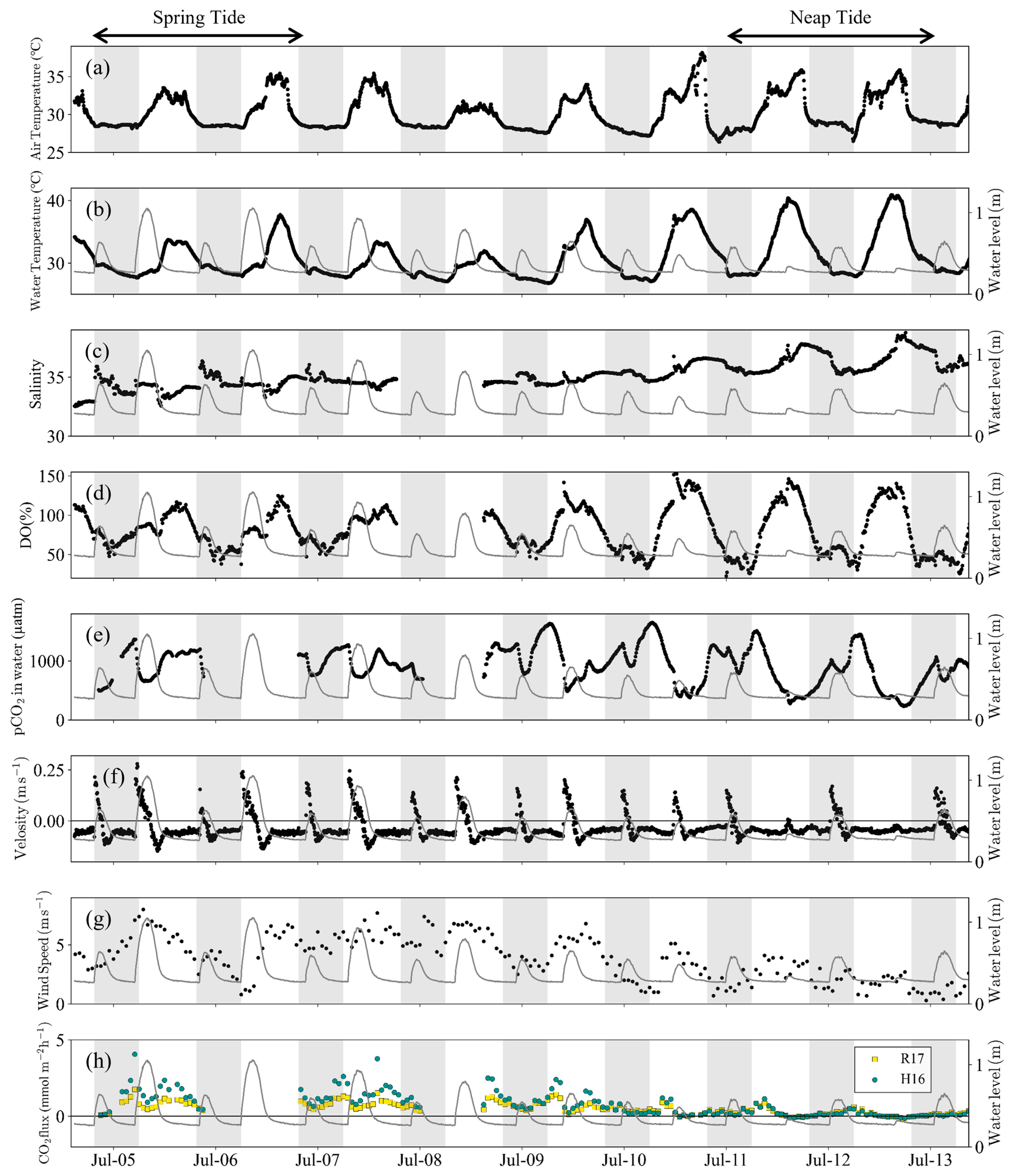
3.2. Water Quality and pCO₂ Change in Front of the Mangrove Forest

The continuous observation data of the water quality in front of the mangrove forest delineated distinct cyclic oscillations. Air and water temperature showed pronounced diurnal oscillations, reaching a maximum around 15:00 (Figure 2a,b). There was no statistically significant difference in air temperature between spring and neap tides (p > 0.05, t-test), while water temperature showed a significant difference (p < 0.0001, t-test). The mean salinity was 34.19 ± 0.74 during the spring tide but increased to 36.42 ± 0.94 during the neap, a significant difference (p < 0.0001, t-test) (Table S2, Figure 2c).

DO also showed pronounced diurnal oscillations (Figure 2d). The mean DO was 81.90 ± 19.72% during the spring tide, whereas it amounted to 75.33 ± 36.3% during the neap tide, displaying a significant difference (p < 0.01, t-test) (Table S2). The standard deviation was particularly large during the neap tide, with a maximum DO value of 124.84% during the spring tide, but reaching 146.23% during the neap tide, indicating oversaturation due to photosynthesis. In contrast to DO, pCO₂ exhibited semi-diurnal oscillations following the tidal cycle (Figure 2e). The mean pCO₂ value over the entire period was 923 ± 318 μatm, with the highest readings typically recorded during low tide (Figure 2e). After 10th July, however, pCO₂ decreased during the day despite low tide (Figure 2e). DO was oversaturated at this time (Figure 2d).

The mean CO₂ flux from water to air was 0.50 ± 0.38 mmol m⁻² h⁻¹ for the R17 model and 0.75 ± 0.76 mmol m⁻² h⁻¹ for the H16 model (Figure 2h). The mean CO₂ flux derived from both models was 0.63 ± 0.62 mmol m⁻² h⁻¹. Following Equation (1), the CO₂ flux is delineated by the gas exchange coefficient, solubility, and the differential pCO₂ existing between the atmosphere and the water. Wind speed, water depth, and current velocity, which are explanatory variables for the gas exchange coefficient, decreased from the spring to neap tides (Figure 2f,g). The mean values of pCO₂ were 954 ± 258 μatm during the spring tide and 785 ± 340 μatm during the neap tide, representing a significant difference (p < 0.0001, t-test). Consequently, the mean CO₂ flux was 1.09 ± 0.75 mmol m⁻² h⁻¹ during the spring tide and 0.18 ± 0.23 mmol m⁻² h⁻¹ during the neap tide (p < 0.0001, t-test) (Figure 2h).

3.3. Diurnal Variation of TA, DIC, and DOC

During the spring tide, TA, DIC, DOC, and δ¹³C_DIC values in front of the mangrove forest varied with the change in tidal level (Figure 3). During the neap tide, TA, DIC, and DOC tended to increase at low tide, albeit with less conspicuous dynamics than those observed during the spring tide (Figure 3). There were no significant differences in TA, DIC, DOC, and δ¹³C_DIC values between the spring and neap tides (p > 0.05, w-test). It is noteworthy that the lowest δ¹³C_DIC values were recorded at −5.64‰ during the spring tide and −4.97‰ during the neap tide, indicative of a lower δ¹³C_DIC value at low tide during the spring tide (Table S2).

The water inflow into the mangrove forest on the Yubu coast corresponded to the tidal range, with a maximum of approximately 10 m³ s⁻¹ during the spring tide and 2.5 m³ s⁻¹ during the neap tide (Figure 3). The water exchange rate amounted to 12,906 m³ d⁻¹ during the spring tide and 13,665 m³ d⁻¹ during the neap tide. TA, DIC, and DOC exports, when weighted according to the surface area of the mangrove forest (0.113 km²) were estimated at 36 ± 26 mmol m⁻² d⁻¹, 42 ± 39 mmol m⁻² d⁻¹, 10 ± 9 mmol m⁻² d⁻¹, respectively (

Table 2. Alkalinity and dissolved carbon export from the mangrove forest to the ocean. Each export value is normalized by the area of the mangrove forest (0.113 km²).

	Spring Tide	Neap Tide	Average
Q (m3 d−1)	12,906	13,665	13,286
ΔTA (μM)	280 ± 250	332 ± 193	306 ± 224
TA flux (mol d−1)	3614 ± 3221	4534 ± 2634	4064 ± 2982
TA export (mmol m−2 d−1)	32 ± 29	40 ± 23	36 ± 26
ΔDIC (μM)	306 ± 342	413 ± 316	359 ± 333
DIC flux (mol d−1)	3947 ± 4415	5639 ± 4315	4772 ± 4430
DIC export (mmol m−2 d−1)	35 ± 39	50 ± 38	42 ± 39
ΔDOC (μM)	88 ± 103	82 ± 47	85 ± 80
DOC flux (mol d−1)	1135 ± 1325	1120 ± 643	1129 ± 1062
DOC export (mmol m−2 d−1)	10 ± 12	10 ± 6	10 ± 9

).

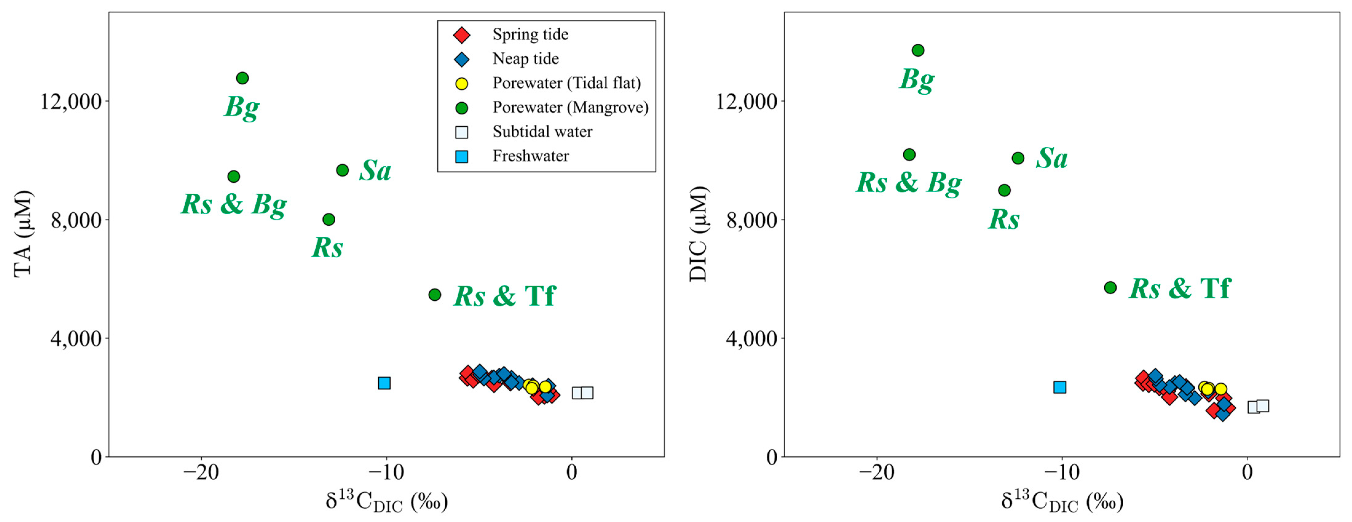
3.4. Spatial Distribution of TA, DIC, and DOC

The mean values of TA, DIC, and DOC in front of the mangrove forest were 2515 ± 254 μM, 2197 ± 360 μM, and 169 ± 55 μM, respectively (Table S2). The TA, DIC, and DOC values within the porewater exhibited substantial variations contingent upon the presence of mangroves. The mean values of TA, DIC, and DOC for mangrove porewater were 9074 ± 2662 μM, 9734 ± 286 μM, and 753 ± 361 μM, respectively, which were extremely high compared to other endmembers (subtidal water, freshwater, and tidal flat porewater) (Table S2 and Figure 4). The mean values of TA, DIC, and DOC of tidal flat porewater were 2370 ± 48 μM, 2305 ± 32 μM, and 117 ± 24 μM, respectively, while the mean and standard deviation were lower than those of mangrove porewater (Table S2 and Figure 4). For mangrove porewater, the mean δ¹³C_DIC value was −13.79 ± 4.4‰, while for tidal flat porewater, it was −2.00 ± 0.3 (Table S2).

The mangrove forest along the Yubu coast exhibits a zonation pattern. The highest values of TA and DIC (12,775 μM and 13,710 μM, respectively) were observed in porewater collected from the landward side of the mangrove forest, where B. gymnorrhiza was the predominant species (blue circle in Figure 1, Figure 4). The highest DOC value (1164 μM) was observed at a site characterized by the dominance of B. gymnorrhiza and R. stylosa (blue and red circle in Figure 1). Porewater collected at the border between the mangrove forest and the tidal flat exhibited lower concentrations for TA, DIC, and DOC, measuring 5767 μM, 5707 μM, and 183 μM, respectively, marking the lowest values among mangrove porewaters (red and yellow circle in Figure 1). The lowest δ¹³C_DIC (−18.26‰) was observed at the site dominated by B. gymnorrhiza and R. stylosa, while the highest (−7.39‰) was recorded at the border between the mangrove forest and the tidal flat (Figure 4).

4. Discussion

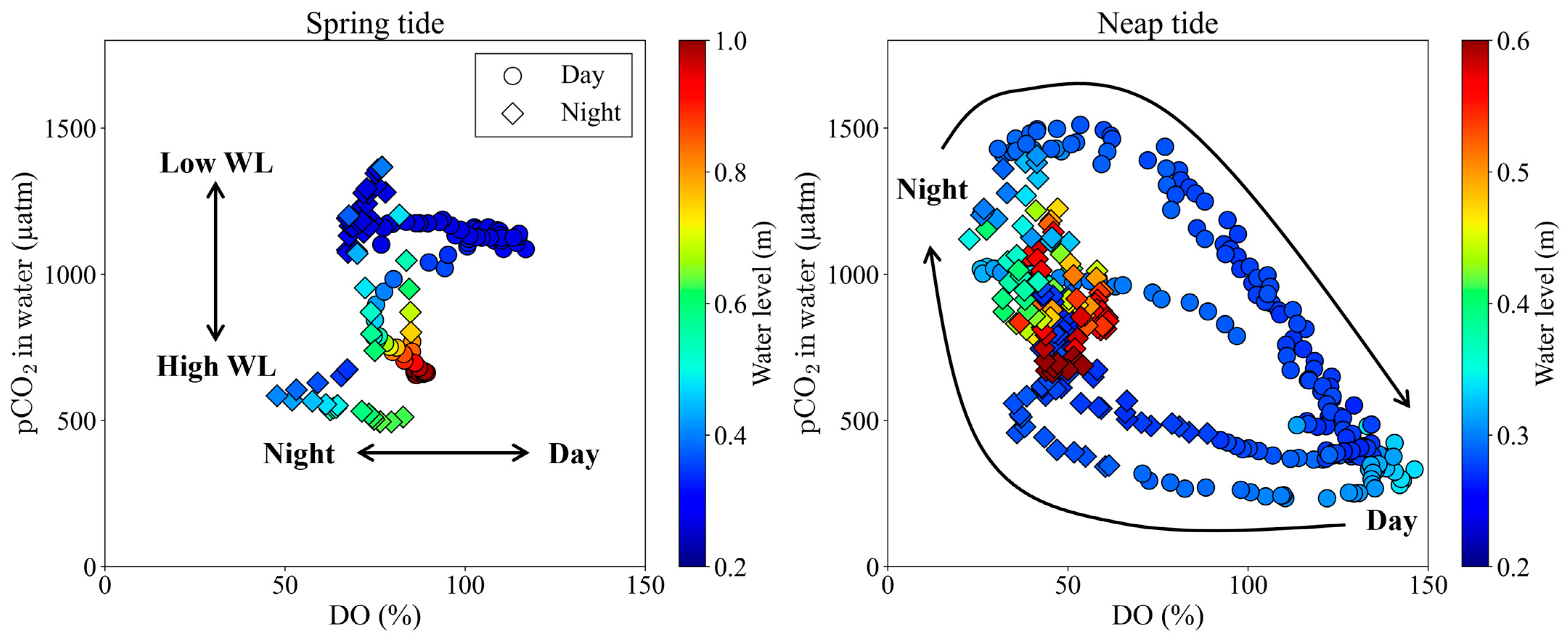
4.1. Controlling Factors of pCO₂ over Spring-Neap Tidal Cycle

On the tidal flat in front of the mangrove forest, DO exhibited a response to diurnal rhythms rather than tidal level changes (Figure 2d). Generally, within mangrove environments, DO is predominantly consumed by the abundant organic matter in the mangrove soils, and both DO and pCO₂ respond to tidal variations [22,23,24,25]. In our investigation, we observed a small decrease in DO during low tide; however, the diurnal modulation of DO showed a nighttime decrease followed by a daytime increase throughout the entire observation period (Figure 2d). This suggests that on the tidal flat in front of the mangrove forest on the Yubu coast, DO varied mainly due to the metabolism of phytoplankton and/or benthic algae rather than consumption in the mangrove soils.

The variability in pCO₂ levels in front of the mangrove forest may be attributed to the dynamics of photosynthesis and respiration in the water, in addition to the export of porewater from the mangrove soil. Generally, pCO₂ levels in mangrove adjacent waters become extremely high due to the export of porewater from the soil by tidal pumping [6,7,8,9,10,41,42,43]. Consequently, pCO₂ in mangrove adjacent waters typically reaches its maximum during low tide. However, the outcomes of this investigation demonstrate an intriguing discrepancy. During the spring tide, pCO₂ in front of the mangrove forest reached its highest value at low tide (Figure 2e and Figure 5). Conversely, during the neap tide, pCO₂ exhibits an increasing trend during the ebb tide, followed by a sharp decrease during daylight hours (Figure 2e and Figure 5). Using multiple regression analysis with pCO₂ as the objective variable and standardized values for water level, DO, and the day/night (dummy variable) as explanatory variables, we observe distinct trends between the spring and neap tides (

Table 3. Multiple regression analysis using pCO₂ as the objective variable and standardized values for water level, DO, and day/night (dummy variable) as explanatory variables. Middle tide means the period between the spring and neap tides.

	Adj. R2	F Statistics p Value	Depth(m)		DO (%)		Day-Night
			Coef.	p Value	Coef.	p Value	Coef.	p Value
Spring tide	0.625	<0.001	−0.72	<0.001	0.27	<0.01	0.01	>0.05
Middle tide	0.651	<0.001	−0.41	<0.001	−0.91	<0.001	0.43	<0.001
Neap tide	0.561	<0.001	0.07	>0.05	−1.05	<0.001	−0.63	<0.001

, Figure 5). During the spring tide, water level exerts the most substantial influence, with a coefficient value of −0.72. The day/night dummy variable was not significantly different and had the lowest influence. This suggests that, during the spring tide, porewater export via tidal pumping, as in other mangrove waters, was a controlling factor in pCO₂ [6,7,8,9,10,41,42,43]. On the contrary, during the neap tide, both DO and the day/night dummy variable significantly contribute, sporting coefficients of −1.05 and −0.63, respectively, while the water level insignificantly influences the pCO₂ dynamics. This suggests that during the neap tide, pCO₂ varied due to photosynthesis and respiration in the tidal flat and subtidal zone.

The divergence in the mechanisms driving pCO₂ during the spring and neap tides may be attributed to alterations in porewater export and offshore water inflow discharge. The inflow of seawater into the mangrove forest was about five times greater during the spring tide than during the neap tide (Figure 3). Furthermore, the δ¹³C_DIC values at low tide were lower during the spring tide than during the neap tide and showed the opposite trend at high tide (Table S2). This suggests that during the spring tide, the variations in carbonate chemistry parameters primarily arise from the water exchange occurring between the mangroves and the ocean. Conversely, during the neap tide, the inflow of open ocean water and the export of porewater become restricted. Consequently, pCO₂ in front of the mangrove forest would have been controlled by photosynthesis and respiration in the tidal flat and subtidal zone.

4.2. Low pCO₂ and CO₂ Efflux in Comparison to the Global Average

The mean pCO₂ in front of the mangrove forest on the Yubu coast was 923 ± 318 μatm, with a corresponding CO₂ efflux to the atmosphere that was 12.3 ± 6.9 (3.4–21.0) mmol m⁻² d⁻¹ using R17 model [36] and 19.1 ± 14.8 (2.6–38.6) mmol m⁻² d⁻¹ using H16 model [37], and the mean value of the two equations was 15.7 ± 10.8 (3.0–29.8) mmol m⁻² d⁻¹. As reviewed by Rosentreter et al. (2018) [25], pCO₂ values in mangrove waters worldwide, encompassing estuaries, bays, and creeks, exhibited a range between 70 to 27,188 μatm, and the mean CO₂ efflux to the atmosphere was notably higher at 56.5 ± 8.9 mmol m⁻² d⁻¹, surpassing the findings of this study. The pCO₂ values, particularly in the vicinity of mangroves, are recognized for their remarkable elevation, making the results of this research relatively lower when compared to prior studies [6,9,10,23]. As a result of the lower pCO₂, the CO₂ flux was also lower than the global average, and the mangrove front on the Yubu coast acted as a weak source of CO₂.

One reason for the low pCO₂ may be primary production on the tidal flat and subtidal zone. pCO₂ levels in mangrove waters are chiefly influenced by tidal level changes [6,9,10]. In the case of Iriomote Island, where the principal lunar semidiurnal component predominantly governs the tidal cycle, tide levels exhibit a nearly semi-diurnal cycle, encompassing both day and night. By comparing pCO₂ values during the day and night, it was evident that daytime pCO₂ was notably lower (p < 0.0001, t-test) (Table S2). The surface water surrounding Iriomote Island has a TA of roughly 2250 μM and a DIC of roughly 1900 μM [44,45]. The mean TA and DIC values in front of the mangrove forest during high tide were 2123 ± 137 μM and 1599 ± 92 μM for the diurnal period-impacted water, while they measured 2321 ± 76 μM and 2100 ± 92 μM for the nocturnal period-impacted water (Figure 3). This pattern suggests that the abundant photosynthesis occurring in the tidal flat and subtidal zone greatly diminished the concentrations of TA and DIC. In particular, the DIC levels were notably reduced, approximately 2.5 times more than TA. The concentration and ratio of TA and DIC determine the variability in pCO₂. The extensive primary production in the tidal flat and subtidal zone potentially led to a decrease in DIC, consequently suppressing the elevation of pCO₂.

Another reason for the low pCO₂ may be the comparatively limited export of porewater from the mangrove soils. For nighttime pCO₂, which is not affected by photosynthesis, the mean value was 976 ± 261 μatm (Table S2), lower than that reported values near the mangrove adjacent waters in riverine mangroves [6,9,10,23]. There are two possible reasons for the small increase in pCO₂ in front of the mangrove forest: (1) greater dilution by seawater or (2) less porewater export. The absence of elevated pCO₂ in mangrove adjacent waters has been reported in the past and was attributed to the inflow of abundant seawater [46]. If the increase in pCO₂ was suppressed by dilution with seawater, the increase in carbonate chemistry parameters should be less during the spring tide, when seawater inflow is higher, than during the neap tide. However, in this study, there was no significant difference in TA and DIC between the spring and neap tides, and pCO₂ was higher during the spring tide than the neap tide (Table S2). Therefore, it is unlikely that dilution with seawater suppressed the increase in pCO₂. The reason for the lower pCO₂ in front of the mangrove forest may have been limited porewater export from the mangrove soils. The TA and DIC values of the porewater in the mangrove soils were extremely high, indicating advanced mineralization of the organic matter deposited in the mangrove soils (Table S2, Figure 4). In many mangrove forests, mangrove-derived organic matter is deposited at depths greater than 1 m below the surface [3,4]. In contrast, in the mangrove forest on the Yubu coast, mangrove-derived organic matter was only deposited to a depth of about 20~30 cm (Figure S4). This may have led to a limited accumulation of mangrove-derived porewater, thus suppressing the escalation of carbonate chemistry parameters in front of the mangrove forest.

One of the indicators of porewater export in mangrove waters is δ¹³C_DIC [23,47,48]. The δ¹³C_DIC in mangrove porewater is substantially lower than that in offshore water, resulting in a lower δ¹³C_DIC value during low tide when pCO₂ becomes high [23,47,48]. In this study, the mean δ¹³C_DIC of porewater within the mangrove soil was notably low at −13.79 ± 4.45 (−18.26~−7.39) ‰, whereas the TA and DIC exhibited extremely high concentrations (Table S2 and Figure 4). However, the mean δ¹³C_DIC in front of the mangrove forest was −3.45 ± 1.49 (−5.64~−1.08) ‰, higher than the −10.34 ± 2.1‰ reported by Taillardat et al. (2018) [23] and the −7.8 ± 5.4‰ reported by Ray et al. (2021) [48]. Furthermore, during low tide, the TA and DIC values in front of the mangrove forest were lower than these reported values. This implies that the export of porewater to the mangrove front was relatively restricted.

In this study, pCO₂ and CO₂ efflux in front of the mangrove forest may have been effectively suppressed due to two key factors: (1) the abundant primary production in the tidal flat and subtidal zone, and (2) the limited export of porewater from the mangroves. In particular, during ebb tides, when pCO₂ typically increases due to porewater export from mangrove soils, a decrease in pCO₂ was observed (Figure 2e). This means that photosynthesis on the tidal flat offsets the increase in pCO₂ caused by the export of porewater from the mangrove soil. Therefore, the tidal flat adjacent to the mangrove forest on the Yubu coast may act as a buffer zone to mitigate the increase in pCO₂, resulting in much of the exported DIC being stored in the ocean.

4.3. Lateral TA, DIC, and DOC Exports from Mangroves to the Ocean

The lateral export of TA and DIC from mangroves to the ocean is considered to be the largest carbon sink, accounting for approximately 63% of the greenhouse gases absorbed by mangrove ecosystems, exceeding their burial rate in the soil [11]. Especially, under conditions where TA is abundantly supplied to the ocean, it may enhance the uptake of atmospheric CO₂ into the ocean [13,14]. On the Yubu coast, the lateral export of TA, DIC, and DOC from the mangrove forests to the ocean was 36 ± 26 mmol m⁻² d⁻¹, 42 ± 39 mmol m⁻² d⁻¹, and 10 ± 9 mmol m⁻² d⁻¹, respectively (Table 2). The TA, DIC, and DOC exports were relatively lower than the global average (TA: 120 ± 182 mmol m⁻² d⁻¹, DIC: 174 ± 213 mmol m⁻² d⁻¹, DOC: 24 ± 25 mmol m⁻² d⁻¹) (

Table 4. Comparison of lateral TA, DIC, and DOC export between this study and selected mangroves around the world (mmol m⁻² d⁻¹).

Location	Target	TA	DIC	DOC	Reference
Yubu Coast, Japan	Spring tide	32 ± 29	35 ± 39	10 ± 12	This study
Yubu Coast, Japan	Neap tide	40 ± 23	50 ± 38	10 ± 6	This study
Fukido River, Japan	Winter	NA	113	17	[49]
Fukido River, Japan	Summer	NA	279	72	[49]
Yutsun River, Japan	River mouth	363	179	66	[26]
Katunggan It Ibajay Ecopark, Philippines	Estuary flux	NA	361 ± 185	16.5 ± 1.7	[48]
Palau, Micronesia	Creek1	48 ± 17	79 ± 28	35 ± 12	[50]
Palau, Micronesia	Creek2	6 ± 5	10 ± 4	8 ± 3	[50]
Can Gio, Vietnam	Symmetric tidal cycle	NA	352 ± 34	21 ± 2	[43]
Can Gio, Vietnam	Asymmetric tidal cycle	NA	678 ± 79	68 ± 8	[43]
Darwin, Australia	Creek	116	85	NA	[13]
Hinchinbrook Island, Australia	Creek	21	22	NA	[13]
Seventeen Seventy, Australia	Creek	81	−97	NA	[13]
Jacobs Well, Australia	Creek	12	83	NA	[13]
Newcastle, Australia	Creek	116	77	NA	[13]
Barwon Heads, Australia	Creek	−1	−3	NA	[13]
Watson Inlet, Australia	Creek	310	440	25	[51]
Chinaman Inlet, Australia	Creek	46	120	0	[51]
Had Head, Australia	Wet Season	27 ± 5	24 ± 5	14 ± 3	[52]
Had Head, Australia	Dry Season	19 ± 4	16 ± 3	3 ± 1	[52]
Gulf of Carpentaria, Australia	Alive mangrove	519–950	584–1050	17	[53]
Gulf of Carpentaria, Australia	Dead mangrove	254–599	291–605	20	[53]
Coffs Creek, Australia	Creek	2.2 ± 1.9	2.2 ± 1.5	−0.3± 1.0	[54]
Evans Head, Australia	Creek	12 ± 6	12 ± 6	2 ± 2	[54]
Everglades, USA	SharkTREx 3	NA	269 ± 19	68 ± 4	[55]
Everglades, USA	SharkTREx 5	NA	253 ± 8	39 ± 1	[55]
Everglades, USA	Shark River	97	142	39	[22]
Amazon, Brazil	Estuary	15 ± 8	20 ± 14	0.3 ± 10	[56]

). This is thought to be due to the low accumulation of mangrove-derived organic matter in the soils on the Yubu coast, which also suppressed the export of alkalinity and dissolved carbon to the ocean (Figure S4).

The lateral export of TA and DIC to the ocean was greater during the neap tide than during the spring tide (Table 4). Taillardad et al. (2018) reported a sharp increase in carbonate chemistry parameters after an asymmetric tide (neap tide) with small tidal amplitude, within a lunar tidal cycle of about 28 days in a meso-tidal area in Vietnam [23,43]. Therefore, DIC and DOC export to the ocean after an asymmetric tide (neap tide) exceeded the symmetric tidal cycle (spring tide). In this study, both water discharge (Q) and ΔTA and ΔDIC were greater during the neap tide than during the spring tide (Table 2). On the Yubu coast, water exchange perpendicular to the mangroves due to tidal variations was almost zero during both spring and neap tides due to the lack of water inflow from behind the mangrove forest (Table S1). Water depth and current velocity in the tidal pool during the tidal flat exposure periods were not significantly different between the spring and neap tides (p > 0.05, t-test) (Figure 2f). Although not as pronounced as in Taillardad et al. (2018) [23,43], ΔTA and ΔDIC were higher during the neap tide than during the spring tide. These suggest that more TA and DIC was exported to the ocean during the neap tide due to the longer exposure period of the tidal flat. The DIC/TA export ratio in this study was 1.17 ± 0.08, which was lower than the global average of 1.41 ± 1.39. This means that compared to other mangrove sites around the world, the DIC exported from the Yubu coast remains in the ocean. A mangrove forest in the same region showed similar trends [26]. This suggests that most of the DIC exported to the ocean from Japanese mangroves, which are at the northern limit of their distribution in the Indo-Pacific region, may be stored in the ocean for a long time.

5. Conclusions

In this study, we investigated the semi-monthly pCO₂ variations on a tidal flat adjacent to a fringe mangrove forest, located at the northern limit of mangrove distribution in the Indo-Pacific region and the export of TA, DIC, and DOC to the ocean. We reported the following three findings:

(1)

Semi-monthly pCO₂ variations on the tidal flat in the mangrove front were controlled by the tidal level during spring tide and by photosynthesis and respiration on the tidal flat during neap tide (Table 3 and Figure 5). This means that during neap tide, photosynthesis on the tidal flat offset the increase in pCO₂ caused by the porewater export from the mangrove soil.

(2)

The pCO₂ and CO₂ efflux in front of the mangrove forest was much lower than the global average, and it may have been effectively suppressed by the primary production in the tidal flat and the limited export of porewater from the mangroves.

(3)

On the Yubu coast, the DIC/TA export ratio was 1.17 ± 0.08, which was lower than the global average of 1.41 ± 1.39, indicating that the DIC exported from the Yubu coast remains in the ocean compared to other mangrove sites around the world (Table 4).

References

1. Nellemann, C.; Corcoran, E.; Duarte, C.M.; Valdrés, L.; Young, C.D.; Fonseca, L.; Grimsditch, G. Blue Carbon: The Role of Healthy Oceans in Binding Carbon; UN Environment, GRID-Arendal: Arendal, Norway, 2009. [Google Scholar]
2. Howard, J.; Sutton-Grier, A.; Herr, D.; Kleypas, J.; Landis, E.; Mcleod, E.; Pidgeon, E.; Simpson, S. Clarifying the Role of Coastal and Marine Systems in Climate Mitigation. Front. Ecol. Environ. 2017, 15, 42–50. [Google Scholar] [CrossRef]
3. Duarte, C.M.; Middelburg, J.J.; Caraco, N. Major Role of Marine Vegetation on the Oceanic Carbon Cycle. Biogeosciences 2005, 2, 1–8. [Google Scholar] [CrossRef]
4. Duarte, C.M.; Losada, I.J.; Hendriks, I.E.; Mazarrasa, I.; Marbà, N. The Role of Coastal Plant Communities for Climate Change Mitigation and Adaptation. Nat. Clim. Chang. 2013, 3, 961–968. [Google Scholar] [CrossRef]
5. Stieglitz, T.C.; Clark, J.F.; Hancock, G.J. The Mangrove Pump: The Tidal Flushing of Animal Burrows in a Tropical Mangrove Forest Determined from Radionuclide Budgets. Geochim. Cosmochim. Acta 2013, 102, 12–22. [Google Scholar] [CrossRef]
6. Chen, X.; Santos, I.R.; Call, M.; Reithmaier, G.M.S.; Maher, D.; Holloway, C.; Wadnerkar, P.D.; Gómez-Álvarez, P.; Sanders, C.J.; Li, L. The Mangrove CO2 Pump: Tidally Driven Pore-water Exchange. Limnol. Oceanogr. 2021, 66, 1563–1577. [Google Scholar] [CrossRef]
7. Borges, A.V.; Djenidi, S.; Lacroix, G.; Théate, J.; Delille, B.; Frankignoulle, M. Atmospheric CO2 flux from Mangrove Surrounding Waters. Geophys. Res. Lett. 2003, 30, 1558. [Google Scholar] [CrossRef]
8. Maher, D.T.; Santos, I.R.; Golsby-Smith, L.; Gleeson, J.; Eyre, B.D. Groundwater-Derived Dissolved Inorganic and Organic Carbon Exports from a Mangrove Tidal Creek: The Missing Mangrove Carbon Sink? Limnol. Oceanogr. 2013, 58, 475–488. [Google Scholar] [CrossRef]
9. Call, M.; Maher, D.T.; Santos, I.R.; Ruiz-Halpern, S.; Mangion, P.; Sanders, C.J.; Erler, D.V.; Oakes, J.M.; Rosentreter, J.; Murray, R.; et al. Spatial and Temporal Variability of Carbon Dioxide and Methane Fluxes over Semi-Diurnal and Spring–Neap–Spring Timescales in a Mangrove Creek. Geochim. Cosmochim. Acta 2015, 150, 211–225. [Google Scholar] [CrossRef]
10. Call, M.; Santos, I.R.; Dittmar, T.; de Rezende, C.E.; Asp, N.E.; Maher, D.T. High Pore-Water Derived CO2 and CH4 Emissions from a Macro-Tidal Mangrove Creek in the Amazon Region. Geochim. Cosmochim. Acta 2019, 247, 106–120. [Google Scholar] [CrossRef]
11. Maher, D.T.; Call, M.; Santos, I.R.; Sanders, C.J. Beyond Burial: Lateral Exchange Is a Significant Atmospheric Carbon Sink in Mangrove Forests. Biol. Lett. 2018, 14, 20180200. [Google Scholar] [CrossRef]
12. Santos, I.R.; Burdige, D.J.; Jennerjahn, T.C.; Bouillon, S.; Cabral, A.; Serrano, O.; Wernberg, T.; Filbee-Dexter, K.; Guimond, J.A.; Tamborski, J.J. The Renaissance of Odum’s Outwelling Hypothesis in “Blue Carbon” Science. Estuar. Coast. Shelf Sci. 2021, 255, 107361. [Google Scholar] [CrossRef]
13. Sippo, J.Z.; Maher, D.T.; Tait, D.R.; Holloway, C.; Santos, I.R. Are Mangroves Drivers or Buffers of Coastal Acidification? Insights from Alkalinity and Dissolved Inorganic Carbon Export Estimates across a Latitudinal Transect. Glob. Biogeochem. Cycles 2016, 30, 753–766. [Google Scholar] [CrossRef]
14. Saderne, V.; Fusi, M.; Thomson, T.; Dunne, A.; Mahmud, F.; Roth, F.; Carvalho, S.; Duarte, C.M. Total Alkalinity Production in a Mangrove Ecosystem Reveals an Overlooked Blue Carbon Component. Limnol. Oceanogr. Lett. 2021, 6, 61–67. [Google Scholar] [CrossRef]
15. Macreadie, P.I.; Anton, A.; Raven, J.A.; Beaumont, N.; Connolly, R.M.; Friess, D.A.; Kelleway, J.J.; Kennedy, H.; Kuwae, T.; Lavery, P.S.; et al. The Future of Blue Carbon Science. Nat. Commun. 2019, 10, 3998. [Google Scholar] [CrossRef] [PubMed]
16. Mamidala, H.P.; Ganguly, D.; Purvaja, R.; Singh, G.; Das, S.; Rao, M.N.; Kazip Ys, A.; Arumugam, K.; Ramesh, R. Interspecific Variations in Leaf Litter Decomposition and Nutrient Release from Tropical Mangroves. J. Environ. Manag. 2023, 328, 116902. [Google Scholar] [CrossRef] [PubMed]
17. Chen, X.; Zhang, F.; Lao, Y.; Wang, X.; Du, J.; Santos, I.R. Submarine Groundwater Discharge-Derived Carbon Fluxes in Mangroves: An Important Component of Blue Carbon Budgets? J. Geophys. Res. C Oceans 2018, 123, 6962–6979. [Google Scholar] [CrossRef]
18. Alongi, D.M. Lateral Export and Sources of Subsurface Dissolved Carbon and Alkalinity in Mangroves: Revising the Blue Carbon Budget. J. Mar. Sci. Eng. 2022, 10, 1916. [Google Scholar] [CrossRef]
19. Shoji, J.; Tomiyama, T. Influence of Vegetation Coverage on Dissolved Oxygen Concentration in Seagrass Bed in the Seto Inland Sea: Possible Effects on Fish Nursery Function. Estuaries Coasts 2023, 46, 1098–1109. [Google Scholar] [CrossRef]
20. Smith, K.J.; Able, K.W. Dissolved Oxygen Dynamics in Salt Marsh Pools and Its Potential Impacts on Fish Assemblages. Mar. Ecol. Prog. Ser. 2003, 258, 223–232. [Google Scholar] [CrossRef]
21. Dubuc, A.; Waltham, N.; Malerba, M.; Sheaves, M. Extreme Dissolved Oxygen Variability in Urbanised Tropical Wetlands: The Need for Detailed Monitoring to Protect Nursery Ground Values. Estuar. Coast. Shelf Sci. 2017, 198, 163–171. [Google Scholar] [CrossRef]
22. Reithmaier, G.M.S.; Ho, D.T.; Johnston, S.G.; Maher, D.T. Mangroves as a Source of Greenhouse Gases to the Atmosphere and Alkalinity and Dissolved Carbon to the Coastal Ocean: A Case Study from the Everglades National Park, Florida. J. Geophys. Res. Biogeosci. 2020, 125, e2020JG005812. [Google Scholar] [CrossRef]
23. Taillardat, P.; Ziegler, A.D.; Friess, D.A.; Widory, D.; Truong Van, V.; David, F.; Thành-Nho, N.; Marchand, C. Carbon Dynamics and Inconstant Porewater Input in a Mangrove Tidal Creek over Contrasting Seasons and Tidal Amplitudes. Geochim. Cosmochim. Acta 2018, 237, 32–48. [Google Scholar] [CrossRef]
24. Ho, D.T.; Ferrón, S.; Engel, V.C.; Anderson, W.T.; Swart, P.K.; Price, R.M.; Barbero, L. Dissolved Carbon Biogeochemistry and Export in Mangrove-Dominated Rivers of the Florida Everglades. Biogeosciences 2017, 14, 2543–2559. [Google Scholar] [CrossRef]
25. Rosentreter, J.A.; Maher, D.T.; Erler, D.V.; Murray, R.; Eyre, B.D. Seasonal and Temporal CO2 Dynamics in Three Tropical Mangrove Creeks—A Revision of Global Mangrove CO2 Emissions. Geochim. Cosmochim. Acta 2018, 222, 729–745. [Google Scholar] [CrossRef]
26. Akhand, A.; Watanabe, K.; Chanda, A.; Tokoro, T.; Chakraborty, K.; Moki, H.; Tanaya, T.; Ghosh, J.; Kuwae, T. Lateral Carbon Fluxes and CO2 Evasion from a Subtropical Mangrove-Seagrass-Coral Continuum. Sci. Total Environ. 2021, 752, 142190. [Google Scholar] [CrossRef] [PubMed]
27. Ewel, K.; Twilley, R.; Ong, J. Different Kinds of Mangrove Forests Provide Different Goods and Services. Glob. Ecol. Biogeogr. Lett. 1998, 7, 83–94. [Google Scholar] [CrossRef]
28. Woodroffe, C.D.; Rogers, K.; McKee, K.L.; Lovelock, C.E.; Mendelssohn, I.A.; Saintilan, N. Mangrove Sedimentation and Response to Relative Sea-Level Rise. Ann. Rev. Mar. Sci. 2016, 8, 243–266. [Google Scholar] [CrossRef] [PubMed]
29. Fujimoto, K.; Hasada, K.; Taniguchi, S.; Furukawa, K.; Ono, K.; Watanabe, S. Progressing influences of sea-level rise to mangrove forests on Iriomote Island, southwestern Japan. In Proceedings of the Annual Meeting of the Association of Japanese Geographers; The Association of Japanese Geographers: Tokyo, Japan, 2018. (In Japanese) [Google Scholar] [CrossRef]
30. Nakamura, W.; Nakamura, Y.; Fujimoto, K.; Suzuki, T.; Higa, H. Analysis on Mangroves Distribution Change over the last 40 Years by using RGB Images of Aira River Mouth in Iriomote Island, Japan and Effect by Sea Level Rise. J. Japan Soc. Civil Eng. Ser. B2 (Coastal Eng.) 2021, 77, I_925–I_930. (In Japanese) [Google Scholar] [CrossRef]
31. Miyagi, T.; Miyagi, F.; Baba, S. The idea and significance of non-disturbed corer“Geoslicer NM series”for mangrove forest-floor investigation. Mangrove Sci. 2023, 14, 15–20. (In Japanese) [Google Scholar]
32. Endo, T.; Tanaka, T.; Otani, S.; Fujita, T.; Yamoch, S. Validity Verification of Measurement Method of Carbon Dioxide Concentration in Water using Water-resistant Breathable Tube. J. Jpn. Soc. Civ. Eng. Ser. B2 2013, 69, I_1251–I_1255. (In Japanese) [Google Scholar] [CrossRef]
33. Dickson, A.G.; Sabine, C.L.; Christian, J.R. Guide to Best Practices for Ocean CO2 Measurements; North Pacific Marine Science Organization: Sidney, BC, Canada, 2007; 191p. [CrossRef]
34. Torres, M.E.; Mix, A.C.; Rugh, W.D. Precise Δ13C Analysis of Dissolved Inorganic Carbon in Natural Waters Using Automated Headspace Sampling and Continuous-flow Mass Spectrometry. Limnol. Oceanogr. Methods 2005, 3, 349–360. [Google Scholar] [CrossRef]
35. Weiss, R.F. Carbon Dioxide in Water and Seawater: The Solubility of a Non-Ideal Gas. Mar. Chem. 1974, 2, 203–215. [Google Scholar] [CrossRef]
36. Rosentreter, J.A.; Maher, D.T.; Ho, D.T.; Call, M.; Barr, J.G.; Eyre, B.D. Spatial and Temporal Variability of CO2 and CH4 Gas Transfer Velocities and Quantification of the CH4 Microbubble Flux in Mangrove Dominated Estuaries. Limnol. Oceanogr. 2017, 62, 561–578. [Google Scholar] [CrossRef]
37. Ho, D.T.; Coffineau, N.; Hickman, B.; Chow, N.; Koffman, T.; Schlosser, P. Influence of Current Velocity and Wind Speed on Air-water Gas Exchange in a Mangrove Estuary. Geophys. Res. Lett. 2016, 43, 3813–3821. [Google Scholar] [CrossRef]
38. Wanninkhof, R. Relationship between Wind Speed and Gas Exchange over the Ocean Revisited. Limnol. Oceanogr. Methods 2014, 12, 351–362. [Google Scholar] [CrossRef]
39. Ray, R.; Baum, A.; Rixen, T.; Gleixner, G.; Jana, T.K. Exportation of Dissolved (Inorganic and Organic) and Particulate Carbon from Mangroves and Its Implication to the Carbon Budget in the Indian Sundarbans. Sci. Total Environ. 2018, 621, 535–547. [Google Scholar] [CrossRef]
40. Alling, V.; Porcelli, D.; Mörth, C.-M.; Anderson, L.G.; Sanchez-Garcia, L.; Gustafsson, Ö.; Andersson, P.S.; Humborg, C. Degradation of Terrestrial Organic Carbon, Primary Production and out-Gassing of CO2 in the Laptev and East Siberian Seas as Inferred from Δ13C Values of DIC. Geochim. Cosmochim. Acta 2012, 95, 143–159. [Google Scholar] [CrossRef]
41. Bouillon, S.; Middelburg, J.J.; Dehairs, F.; Borges, A.V.; Abril, G.; Flindt, M.R.; Ulomi, S.; Kristensen, E. Importance of Intertidal Intertidal Sediment Processes and Porewater Exchange on the Water Column Biogeochemistry in a Pristine Mangrove Creek (Ras Dege, Tanzania). Biogeosciences 2007, 4, 311–322. [Google Scholar] [CrossRef]
42. Akhand, A.; Chanda, A.; Manna, S.; Das, S.; Hazra, S.; Roy, R.; Choudhury, S.B.; Rao, K.H.; Dadhwal, V.K.; Chakraborty, K.; et al. A Comparison of CO2 Dynamics and Air-Water Fluxes in a River-Dominated Estuary and a Mangrove-Dominated Marine Estuary. Geophys. Res. Lett. 2016, 43, 11726–11735. [Google Scholar] [CrossRef]
43. Taillardat, P.; Willemsen, P.; Marchand, C.; Friess, D.A.; Widory, D.; Baudron, P.; Truong, V.V.; Nguyễn, T.-N.; Ziegler, A.D. Assessing the Contribution of Porewater Discharge in Carbon Export and CO2 Evasion in a Mangrove Tidal Creek (Can Gio, Vietnam). J. Hydrol. 2018, 563, 303–318. [Google Scholar] [CrossRef]
44. Chen, C.T.A.; Liu, C.T.; Pai, S.C. Variations in Oxygen, Nutrient and Carbonate Fluxes of the Kuroshio Current. La Mer 1995, 33, 161–176. [Google Scholar]
45. Chou, W.-C.; Sheu, D.D.; Chen, C.T.A.; Wen, L.-S.; Yang, Y.; Wei, C.-L. Transport of the South China Sea Subsurface Water Outflow and Its Influence on Carbon Chemistry of Kuroshio Waters off Southeastern Taiwan. J. Geophys. Res. 2007, 112, C12008. [Google Scholar] [CrossRef]
46. Akhand, A.; Chanda, A.; Watanabe, K.; Das, S.; Tokoro, T.; Chakraborty, K.; Hazra, S.; Kuwae, T. Low CO2 Evasion Rate from the Mangrove-Surrounding Waters of the Sundarbans. Biogeochemistry 2021, 153, 95–114. [Google Scholar] [CrossRef]
47. Ray, R.; Thouzeau, G.; Walcker, R.; Vantrepotte, V.; Gleixner, G.; Morvan, S.; Devesa, J.; Michaud, E. Mangrove-Derived Organic and Inorganic Carbon Exchanges Between the Sinnamary Estuarine System (French Guiana, South America) and Atlantic Ocean. J. Geophys. Res. Biogeosci. 2020, 125, e2020JG005739. [Google Scholar] [CrossRef]
48. Ray, R.; Miyajima, T.; Watanabe, A.; Yoshikai, M.; Ferrera, C.M.; Orizar, I.; Nakamura, T.; San Diego-McGlone, M.L.; Herrera, E.C.; Nadaoka, K. Dissolved and Particulate Carbon Export from a Tropical Mangrove-Dominated Riverine System. Limnol. Oceanogr. 2021, 66, 3944–3962. [Google Scholar] [CrossRef]
49. Ohtsuka, T.; Onishi, T.; Yoshitake, S.; Tomotsune, M.; Kida, M.; Iimura, Y.; Kondo, M.; Suchewaboripont, V.; Cao, R.; Kinjo, K.; et al. Lateral Export of Dissolved Inorganic and Organic Carbon from a Small Mangrove Estuary with Tidal Fluctuation. Forests 2020, 11, 1041. [Google Scholar] [CrossRef]
50. Call, M.; Sanders, C.J.; Macklin, P.A.; Santos, I.R.; Maher, D.T. Carbon Outwelling and Emissions from Two Contrasting Mangrove Creeks during the Monsoon Storm Season in Palau, Micronesia. Estuar. Coast. Shelf Sci. 2019, 218, 340–348. [Google Scholar] [CrossRef]
51. Faber, P.A.; Evrard, V.; Woodland, R.J.; Cartwright, I.C.; Cook, P.L.M. Pore-Water Exchange Driven by Tidal Pumping Causes Alkalinity Export in Two Intertidal Inlets. Limnol. Oceanogr. 2014, 59, 1749–1763. [Google Scholar] [CrossRef]
52. Sadat-Noori, M.; Maher, D.T.; Santos, I.R. Groundwater Discharge as a Source of Dissolved Carbon and Greenhouse Gases in a Subtropical Estuary. Estuaries Coasts 2016, 39, 639–656. [Google Scholar] [CrossRef]
53. Sippo, J.Z.; Maher, D.T.; Schulz, K.G.; Sanders, C.J.; McMahon, A.; Tucker, J.; Santos, I.R. Carbon Outwelling across the Shelf Following a Massive Mangrove Dieback in Australia: Insights from Radium Isotopes. Geochim. Cosmochim. Acta 2019, 253, 142–158. [Google Scholar] [CrossRef]
54. Santos, I.R.; Maher, D.T.; Larkin, R.; Webb, J.R.; Sanders, C.J. Carbon Outwelling and Outgassing vs. Burial in an Estuarine Tidal Creek Surrounded by Mangrove and Saltmarsh Wetlands. Limnol. Oceanogr. 2019, 64, 996–1013. [Google Scholar] [CrossRef]
55. Volta, C.; Ho, D.T.; Maher, D.T.; Wanninkhof, R.; Friederich, G.; Del Castillo, C.; Dulai, H. Seasonal Variations in Dissolved Carbon Inventory and Fluxes in a Mangrove-dominated Estuary. Glob. Biogeochem. Cycles 2020, 34, e2019GB006515. [Google Scholar] [CrossRef]
56. Cabral, A.; Dittmar, T.; Call, M.; Scholten, J.; de Rezende, C.E.; Asp, N.; Gledhill, M.; Seidel, M.; Santos, I.R. Carbon and Alkalinity Outwelling across the Groundwater-Creek-Shelf Continuum off Amazonian Mangroves. Limnol. Oceanogr. Lett. 2021, 6, 369–378. [Google Scholar] [CrossRef]
Figure 1. Location map and sampling sites on the Yubu coast, Iriomote Island, Japan. The blue star indicates the station where we installed a mooring system and collected water samples from both spring and neap tides. The circles and crosses indicate the site where we collected porewater and surface soil samples, respectively. The squares indicate the site where we collected end-member water samples. The green area and white line indicate mangrove distribution and freshwater input, respectively. The original pictures are from the Geospatial Information Authority in Japan.
Jmse 11 02356 g001
Figure 2. Time series observations of (a) is air temperature, (b) is water temperature, (c) is salinity, (d) is DO, (e) is pCO2, (f) is current velocity, (g) is wind speed, and (h) is CO2 flux. Grey lines indicate water level change. The grey bands represent the nighttime portion of the diurnal cycle. A positive current velocity means northward flow. A positive CO2 flux value means the CO2 flux from water to air. R17 and H16 indicate different gas transfer velocity models by Rosentreter et al. (2017) [36] and Ho et al. (2016) [37], respectively.
Jmse 11 02356 g002
Figure 3. Diurnal variations in TA, DIC, DOC, and δ13CDIC at the blue star in Figure 1 and their lateral fluxes on the Yubu coast. The grey and red lines indicate water level change and discharge, respectively. The grey bands represent the nighttime portion of the diurnal cycle. Positive fluxes and discharge mean the input to the mangrove forest.
Jmse 11 02356 g003
Figure 4. The relationship between δ13CDIC vs. TA and DIC for all water samples. Green and yellow circles mean porewater samples in the mangrove and tidal flat, respectively. Bg, Rs, Sa, and Tf represent samples collected around B. gymnorrhiza, R. stylosa, S. alba, and tidal flat dominated areas, respectively (Figure 1).
Jmse 11 02356 g004
Figure 5. The relationship between DO saturation and pCO2 in water both spring and neap tides. Circles and diamonds indicate the data collected during daytime and nighttime, respectively.
Jmse 11 02356 g005