A Bi-Level Programming Approach to Optimize Ship Fouling Cleaning

Abstract

Ship fouling has significant adverse effects on vessel performance and environmental sustainability. Therefore, this research study develops a bi-level programming model to simultaneously optimize cleaning equipment deployment by cleaning service providers in the upper level and cleaning decisions by shipping companies in the lower level. To address the interaction within the bi-level problem, the model is transformed into a single-level formulation using the big-M method. This transformation greatly simplifies the complexity of the computation and reduces computation time. Numerical experiments are conducted using real-world data to evaluate the performance of the proposed models. In addition, sensitivity analyses are performed to investigate the influence of key parameters. The results indicate that cleaning service providers primarily purchase equipment in the first year based on the demand distribution. To maximize profit, they may choose to forgo a portion of the demand. The sensitivity analysis reveals that sacrificing part of the demand can lead to an additional USD 27 million in profits compared with satisfying all demand. Moreover, increasing the cleaning price reduces both demand and equipment purchases but increases total profits. Conversely, increasing purchase costs reduces profits and the total amount of equipment purchased. When service providers can no longer generate profits, they are likely to exit the market. These findings offer valuable insights for service providers and shipping companies in the practical deployment of cleaning equipment and foul cleaning decisions, respectively.

1. Introduction

Maritime shipping is a crucial component of global logistics, responsible for delivering over 80% of global trade by volume in 2022 according to the United Nations Conference on Trade and Development (UNCTAD). During shipping voyages, various marine organisms, such as algae, plants, and small animals, attach to the surface of a ship’s hull, leading to ship fouling. Such ship fouling has significant adverse effects on both vessel performance and environmental sustainability. First, it increases hydrodynamic drag, which in turn increases fuel consumption and greenhouse gas emissions. Utama and Nugroho [1] provide an overview of the relationship between biofouling, ship drag, and fuel consumption. Hakim et al. [2] conclude that fuel consumption increases by about 10% in a year due to marine fouling. Second, ship fouling can facilitate the transport and introduction of non-native species, leading to ecological disturbance and potential damage to marine ecosystems. Fitridge et al. [3] show that a conservative estimate of the direct economic losses caused by biofouling on the aquaculture industry is 5%–10%. Therefore, it is imperative to regularly clean ship hulls to reduce the adverse impacts of biofouling. There are two main approaches to keeping a ship’s hull clean: the first approach is to use antifouling coatings [4], and the second is hull cleaning [5,6]. Antifouling coatings, as the name suggests, involve the application of special coatings to the surface of a ship’s hull to reduce the attachment of pollutants and marine organisms. These coatings typically contain additives that deter biofouling, making the surface of a ship’s hull easier to clean than in the absence of such coatings. Conversely, hull cleaning involves the physical or chemical removal of pollutants and marine organisms that have already attached to the surface of a ship’s hull. Methods used include scraping, high-pressure water cleaning, high-frequency ultrasonic cleaning, and chemical cleaning.

This article primarily focuses on the second approach, that is, the cleaning of a ship’s hull when pollutants and marine organisms are already attached. Those interested in antifouling coatings can refer to references [7,8]. Many countries have issued regulations on biofouling cleaning. For example, New Zealand and Australia require all vessels to carry out hull cleaning within 30 days of arrival in their ports 1. These regulations aim to prevent the spread of invasive species due to contaminated hulls and to maintain the ecological balance of marine ecosystems.

The hull cleaning process involves two parties: cleaning service providers and shipping companies. The former provide cleaning equipment and services, aiming to maximize their profits, whereas the latter decide whether and where to use the cleaning service such that their cost is minimized. To formulate the interaction between the two parties, a bi-level non-linear programming model was developed. In the upper level of the model, the service provider makes decisions regarding the deployment of equipment, considering factors such as service revenue and equipment costs. Meanwhile, in the lower level, shipping companies optimize their cleaning decisions by balancing the cost of fouling cleaning, the additional fuel cost caused by fouling, and the availability of cleaning equipment. The problem is challenging from a computational standpoint due to the interaction between the decisions at both levels and the non-linearity of the lower-level problem. To address the complexity of the problem, the bi-level non-linear model is transformed into a single-level linear model using the big-M method, a mathematical technique used in linear programming to handle constraints with binary decision variables. The transformed problem can be easily solved by the off-the-shelf Gurobi solver (version 10.0), a widely-used software package for linear programming (LP), mixed-integer linear programming (MILP), quadratic programming (QP), mixed-integer quadratic programming (MIQP), and other related optimization problems. Numerical experiments are conducted to compare the performance of the proposed solution method with a heuristic algorithm that iteratively solves the upper-level and lower-level problems in sequence until the upper-level solution remains unchanged. The results demonstrate that the proposed method, which transforms the bi-level model into a single-level model, is well suited to the problem as it significantly speeds up computation compared with the heuristic algorithm. Furthermore, the results of the numerical experiments suggest that cleaning service providers engage in partial demand fulfillment to maximize profit. In addition, it is recommended that equipment procurement be prioritized in the first year. Sensitivity analyses are performed to explore the impact of key parameters. The findings reveal that requiring full demand satisfaction results in a USD 27 million loss in profit for the cleaning service providers. Increases in the purchase cost of equipment also decrease the providers’ profits and potentially lead to some service providers exiting the market. However, increasing cleaning price will increase total profits at the expense of fulfilling only a portion of the demands.

The rest of the paper is organized as follows. Section 2 briefly reviews the related literature. Section 3 describes the problem and formulates it as a bi-level programming model. The solution method is proposed in Section 4, and several numerical experiments are conducted in Section 5. In Section 6, a comprehensive discussion is provided on the limitations of the present research and future directions for further investigation. Finally, the conclusions drawn from the study are summarized in Section 7.

2. Literature Review

This study aims to develop and optimize the fouling cleaning process through the use of a bi-level programming model. To provide a comprehensive understanding of the subject, this literature review mainly focuses on an exploration of the research topic and an examination of the relevant literature pertaining to the chosen model type.

Research on ship fouling has garnered attention for more than 40 years. Evans [9] summarized important findings on the biology of fouling algae, which have proven valuable for the advancement of antifouling technologies. Additionally, Callow [10] provided comprehensive information on various solution methods to combat fouling, encompassing both traditional and modern approaches. These methods include the use of antifouling paints, copper, organo-tin, tributyltin, and fluoropolymers of silicones. Since ship fouling has significant negative impacts on vessel performance and environmental sustainability, there are many studies aimed at quantifying these effects. Townsin [11] elucidated ship speed and power performance penalties caused by slime, shell, and weed separately. Monty et al. [12] assessed the ship drag penalty caused by light calcareous tubeworm fouling. Demirel et al. [13] analyzed the effect of barnacle fouling on ship resistance and powering. Coraddu et al. [14] developed a data-driven digital twin of the ship using information collected from on board sensors to predict the speed losses caused by fouling. Demirel et al. [15] investigated frictional resistance coefficients under a range of representative coating and fouling conditions. Farkas et al. [16] and Song et al. [17] carried out simulations to investigate the impacts of different fouling conditions on different ship types. The results show that the influence can vary significantly amongst different ship types. Farkas, Degiuli, and Martić [18] divided biofouling into soft and hard fouling, where the latter has greater impact. To quantify the influence of hard fouling, they developed a roughness function through simulation to measure the resistance caused by fouling. Erol, Cansoy, and Aybar [19] used data collected from all automation systems instead of noon reports to improve the measurement accuracy of the relationship between fouling and ship performance. In addition to quantifying the impacts, there are also studies investigating the effectiveness of different cleaning methods. Tribou and Swain [20] assessed the effectiveness of grooming with a five-headed rotating brush to clean biofouling. Experiments show that the effectiveness of the tool depends on the fouling condition. Oliveira and Granhag [21] investigated the maximum wall shear stress and jet stagnation pressure that do not cause damage or wear to antifouling coatings. Zhong et al. [22] conducted experiments to verify the feasibility of ultrasonic-enhanced submerged cavitation jets in the cleaning of ship fouling. Given the importance of determining the optimal timing for cleaning methods, several researchers have contributed to this field. Farkas, Degiuli, and Martić [23] address the challenge of rapidly predicting propeller performance with fouled surfaces when making maintenance schedules. Farkas, Degiuli, and Martić [24] also developed a model to rapidly predict the effect of biofouling on a ship’s hydrodynamic performance during maintenance schedule optimization. Georgiev and Garbatov [25] performed conceptual multipurpose vessel design and fleet sizing considering hull form, resistance and propulsion, and other dimensions crucial to vessel design. Degiuli et al. [26] optimized the maintenance schedule for containerships considering fouling penalties under real environmental conditions. While the literature has extensively examined the effects of fouling, cleaning methods, and cleaning schedules, there remains a gap in comprehensive research that simultaneously addresses the optimal locations and timing for ship cleaning, as well as the appropriate number of devices to be deployed.

The problem in this study is formulated as a bi-level model. Bi-level optimization involves two levels of optimization interacting with each other (typically involving a leader in the upper level and a follower in the lower level), where the decisions made in the upper level affect the solution of the lower level and the solution of the lower level in turn influences the objective function or constraints of the upper level. Bi-level programming problems arise in many different applications, such as transportation management [27,28], facility location [29,30,31], and logistics optimization [32,33]. In the shipping industry, many problems are also formulated as bi-level models. Qi, Wang, and Psaraftis [34] conducted a comprehensive review of bi-level optimization models for air emission management in the shipping industry. Wang et al. [35] proposed a novel bi-level model aimed at optimizing the energy consumption of a fleet. The upper-level optimization model determined the loading and speed of each ship, taking into account relevant factors such as port information, the navigational environment, time requirements, and ship parameters. The lower-level problem was formulated as a dynamic model, optimizing energy consumption by considering varied environmental factors and port information. Zhu, Shen, and Shi [36] developed a bi-level multi-objective model for the allocation of carbon emission allowances. In this model, the government acted as the leader initiating the allocation process, while shipping companies served as followers and made decisions regarding carbon emissions within their operations. Yang, Pan, and Wang [37] reconstructed liner shipping networks considering the impacts of two new railway systems built under the one belt one road policy. The upper-level liner shipping company decided shipping routes while the lower-level shippers decided delivery amounts along the routes. Zhuge et al. [38] investigated the effects of different policies regarding vessel speed reduction in a port area. Four policies were compared and two bi-level subsidy design models were formulated. Ziar et al. [39] designed an environmentally friendly intermodal transportation network. The government in the upper level decided the location of dry ports, while the freight carriers in the lower level optimized shipping routes. Wang, Wang, and Zhen [40] optimized the subsidy plan for scrubbers and shore power through a bi-level mixed-integer programming model, where the government at the upper level minimized the total subsidy amount while ship operators at the lower level chose the most cost-effective energy supply. Cai et al. [41] used a bi-level mixed-integer programming model to determine the type and amount of search and rescue equipment allocated to activated stations. Although bi-level models have been widely used in maritime operation optimization involving two decision parties, no research has been conducted to explore ship fouling cleaning when cleaning service providers and ships interact with each other.

In conclusion, this research makes three main contributions:

• This study provides a quantitative approach to optimize the fouling cleaning process, which is a unique contribution compared to the existing literature. By applying mathematical techniques and optimization methods, the present research offers a systematic framework for achieving efficient and effective foul cleaning.
• The present research introduces a bi-level model that incorporates both service providers and demanders. In this model, the upper-level decision makers, who are the service providers, determine the optimal deployment of cleaning equipment, including location, quantity, and timing, in order to maximize total profits. On the other hand, the lower-level decision makers, which are the ships, decide when and where to clean fouling to minimize the total cost. It is important to note that the upper-level deployment decision influences the cleaning decisions of the lower-level ships, while the lower-level decisions also impact the upper-level deployment. This bi-level model allows for the simultaneous optimization of equipment deployment and service purchase decisions. By considering the interactions between these two groups, the study offers comprehensive solutions that address the needs and objectives of both service providers and demanders.
• To enhance computational efficiency, the present research transforms the complex bi-level non-linear problem into a single-level linear problem through the big-M method, which converts the formulation of the lower-level problem into constraints for the upper-level problem. By doing so, the two problems are effectively merged into a single-level optimization problem, which can be solved using linear programming techniques. This transformation simplifies the optimization process and reduces the computational complexity, resulting in faster solution times.

3. Problem Description and Formulation

This section presents problem description and the model formulation. The main nomenclature is summarized in

Table 1. Nomenclature.

Sets
$R$	Set of container shipping routes, indexed by $r$,$r\in R$
$P$	Set of all ports on shipping routes, indexed by $p$,$p\in P$
$S$	Set of homogenous ships, indexed by $s$,$s\in S$
$N$	Planning period, indexed by $n$, $n\in \{1,\dots , \left|N\right|\}$
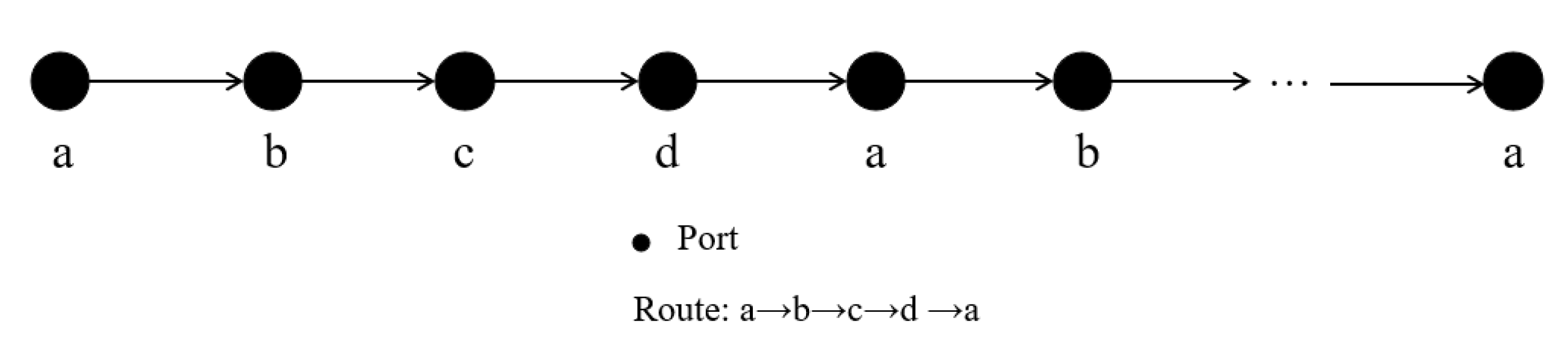
${\Phi }_s$	An ordered set of port–time pairs of ship $s$
${\Phi }_{sk}$	Set of all port–time pairs of ship $s$ at the $k$th year
${\Omega }_s$	Set of all port–time pairs of ship $s$ that have $y_{spt}^{\ast }=1$
${\Omega }_{sk}$	Set of all port–time pairs of ship $s$ that have $y_{spt}^{\ast }=1$ and $365(k-1)<t\le 365k$
${\mathrm{V}}_{spt}$	Set of ships that are in service at port $p$ when ship $s$ arrives at this port at the port–time pair $(p,t)$
${\mathbb{Z}}_0^{+}$	Set of non-negative integers
Parameters
$C^f$	The unit fuel cost (USD/nautical mile)
$C^p$	The cleaning price (USD) at port $p$
$C^e$	The amortized purchasing cost (USD/year) of cleaning equipment
$L_{sp}$	The distance (nautical mile) of the next leg for ship $s$ after visiting port $p$
$D_{sp}$	The dwell time (days) of ship $s$ at port $p$
$\alpha$	The increase in the rate of fouling (kg/m2·day)
$\beta$	The coefficient between fuel consumption growth rate and ship fouling level
${\pi }_{spt}$	The position of port–time pair $(p,t)$ at set ${\Phi }_s$
${\tau }_{spt}$	The position of port–time pair $(p,t)$ at set ${\Omega }_s$
Decision variables
$x_{pn}$	The amount of equipment to be deployed at port $p$ at the beginning of the $n$th year
$y_{spt}$	Binary variable which equals 1 if the ship $s$ cleans fouling at the port–time pair $(p,t)$ or 0 otherwise
$F_{spt}$	The fouling accumulation (kg) on a ship $s$ at port–time pair $(p,t)$

, and additional ones will be introduced whenever necessary.

The present research designs the plan for cleaning equipment deployment and ship fouling cleaning in a liner shipping network with a set of shipping routes, with the set indicated by $R$. Let $N$ be the set of the planning horizon consisting of $\left|N\right|$ time periods, each corresponding to a year. In this context, the route $r\in R$ is defined as a closed loop, serving $\left|P_r\right|$ ports of call and $\left|A_r\right|$ legs, where $\left|A_r\right|=\left|P_r\right|-1$. For instance, the route $r$ can be described by $(a,b,c,d,a)$ where port $a$, $b$, $c$, $d$, and $a$ are the first, second, third, fourth, and fifth port of call, respectively. The voyage from the $i$^th port of call to the ($i+1$)^th port of call is the $i$^th leg. The collection of all ports within these routes forms the set $P$. A fleet of homogeneous ships, denoted as $S$, sails along these routes. Each ship $s\in S$ operates exclusively and repeatedly on a single route, as illustrated in Figure 1. In contrast, a route may accommodate multiple ships with diverse schedules, as depicted in Figure 2. When ship $s$ arrives at port $p$, its time of arrival is recorded as $t$ (measured in days), creating a port–time pair denoted as $(p,t)$. These pairs are arranged in the order of the ship’s ports of call. For any $n\in N$, there is an ordered set ${\Phi }_{sn}$ including all the port–time pairs of ship $s$ in which the time $t$ satisfies $365(n-1)<t\le 365n$. All port–time pairs of ship $s$ during planning period $N$ are combined to form the ordered set ${\Phi }_s$, where ${\Phi }_s={\bigcup }_{n\in N}{\Phi }_{sn}$. It is important to note that all ships accumulate fouling during their voyages. It is assumed that biofouling does not increase while a ship is in motion due to its high speed. However, when a ship remains stationary, such as when floating or at berth, fouling accumulates linearly with time at a rate of $\alpha$. The extent of fouling accumulation on ship $s$ when arriving at a given port–time pair $(p,t)$ is denoted as $F_{spt}$ (kg/m²). For instance, in Figure 1, ship $s$ departs from port $a$ without any fouling on the first day. After three days of sailing, it arrives at port $b$ with no fouling accumulation ($F_{sb4}=0$). However, after spending two days berthed at port $b$, the fouling on the ship increases to $2\alpha$ ($F_{sb4}+2\alpha =2\alpha$). Furthermore, it is assumed that the growth rate of fuel consumption is linearly related to fouling, with a coefficient of $\beta$. For example, considering the fouling of ship $s$ before departing from port $b$ as $2\alpha$, fuel consumption will increase by the proportion of $2\alpha \beta$ when the ship travels from port $b$ to port $c$.

3.1. Bi-Level Decisions

Two parties are involved in the present research: cleaning service providers and ships. The service providers provide fouling cleaning services at different ports with different prices, while ships arriving at a port of call decide whether to purchase the fouling cleaning service from the service providers. The research problem is formulated as a bi-level model. In the upper level, service providers optimize their service deployment strategies. In the lower level, ships, as the customers of fouling cleaning services, optimize their cleaning decisions.

Before introducing the bi-level problem, it should be mentioned that ships are cost-driven, which means that regardless of the deployment plans proposed by service providers, each ship $s$ has its own optimal decisions as to where to use the cleaning service. The decisions are exclusively determined by total costs, as shown in the following model:

$$[\mathrm{P}1] \mathrm{Minimize} {\sum }_{(p,t)\in {\Phi }_s}\left[\left(F_{spt}+\alpha D_{sp}\right)\beta \left(1-y_{spt}\right)C^f{L}_{sp}+C^p{y}_{spt}\right]$$

(1)

subject to

$$F_{spt}=\left(F_{s{p}^{\prime }{t}^{\prime }}+\alpha D_{s{p}^{\prime }}\right)\left(1-y_{s{p}^{\prime }{t}^{\prime }}\right), \forall \left(p,t\right),\left(p^{\prime },t^{\prime }\right)\in {\Phi }_s: {\pi }_{spt}-{\pi }_{s{p}^{\prime }{t}^{\prime }}=1$$

(2)

$$y_{spt}\in \left\{\mathrm{0,1}\right\}, \forall \left(p,t\right)\in {\Phi }_s.$$

(3)

The objective Function (1) minimizes total costs which consist of additional fuel costs incurred by biofouling and cleaning costs. Constraints (2) are a state transition function between two consecutive states. Constraints (3) define $y_{spt}$ to be binary.

Since P1 is deterministic, the optimal solutions $y_{spt}^{\ast }$, $\forall (p,t)\in {\Phi }_s$, $s\in S$ can be easily obtained. For each $y_{spt}^{\ast }=1$, it means that ship $s$ requires a cleaning service when arriving at port–time pair $(p,t)$. Let ${\Omega }_s$ and ${\Omega }_{sk}$ be the set for ship $s$ that includes all port–time pairs $(p,t)$ that have $y_{spt}^{\ast }=1$ and the port–time pairs that have $y_{spt}^{\ast }=1$ and $365(k-1)<t\le 365k$, respectively. Therefore, ${\Omega }_s$ can be regarded as the demand for cleaning services for ship $s$. Having ship demands, the bi-level decision problem can be formulated.

The service providers collectively act as the leader, whose main goal is to maximize profits by designing an optimal deployment plan for cleaning equipment. Their profits are derived from service revenue minus equipment costs. It is worth noting that different prices for cleaning services exist at different ports, while the equipment costs remain the same. Since fouling accumulation occurs over a period of time, the service providers are not required to purchase all the equipment in the first year. Instead, they determine the amount of equipment to be purchased at the beginning of each year ($n$th year) for each port, denoted as $x_{pn}$. Deploying more equipment allows for the servicing of a greater number of ships, thus increasing service revenue. However, it also leads to higher equipment costs. Hence, the service providers need to carefully design the deployment plan to balance between revenue and costs.

On the other hand, the ships, as the followers, determine whether and where to utilize the cleaning service under the given the deployment plan $\overrightarrow{x}$. To maximize the total profits, the deployment plan made by service providers may not be able to serve all demands. Consequently, the ships that cannot be served will not use the cleaning service on the subsequent voyages and instead turn to other techniques, such as antifouling painting. Because ship demands are the best choice based on total costs, any violation will increase total costs, and it is assumed that ships do not accept cost increases. The total demands when ship $s$ arrives at port $p$ at port–time pair $(p,t)$ is denoted as ${|\mathrm{V}}_{spt}|$. Given the deployment plan $\overrightarrow{x}$, the choices of ship $s$ can be modeled as follows:

$$[\mathrm{P}2] Y_s\left(\overrightarrow{x}\right)=\mathrm{a}\mathrm{r}\mathrm{g}\mathrm{m}\mathrm{i}\mathrm{n}{\sum }_{k\in N}{\sum }_{\left(p,t\right)\in {\Omega }_{sk}}\left(\left|{\mathrm{V}}_{spt}\right|+1-{\sum }_{n=1}^k{x}_{pn}\right)y_{spt}$$

(4)

subject to

$$y_{spt}\le y_{s{p}^{\prime }{t}^{\prime }}, \forall \left(p,t\right), \left(p^{\prime },t^{\prime }\right)\in {\Omega }_s:{\tau }_{spt}-{\tau }_{s{p}^{\prime }{t}^{\prime }}=1$$

(5)

$$y_{spt}\in \left\{\mathrm{0,1}\right\}, \forall (p,t)\in {\Omega }_s.$$

(6)

Let $(p,t)\in {\Omega }_s$ be the first pair at which the equipment supply is insufficient to satisfy demands, i.e., $\left|{\mathrm{V}}_{spt}\right|+1>{\sum }_{n=1}^k{x}_{pn}$. In the optimal solution, there will be $y_{s{p}^{\prime }{t}^{\prime }:{\tau }_{s{p}^{\prime }{t}^{\prime }}<{\tau }_{spt}}=1$ and $y_{s{p}^{\prime }{t}^{\prime }:{\tau }_{s{p}^{\prime }{t}^{\prime }}\ge {\tau }_{spt}}=0$. This means that when the port can provide sufficient equipment, the ship $s$ will use the service. Conversely, if the port cannot meet requirements, the ship $s$ will not use the service. Constraints (5) state that the ship will leave the market and turn to other techniques once it cannot be served. Constraints (6) define $y_{spt}$ to be binary.

3.2. Model Formulation

Given the lower-level solution $Y_s\left(\overrightarrow{x}\right)$, $\forall s\in S$, the service providers can maximize total profits by designing the equipment deployment plan as follows:

$$[\mathrm{P}3] \mathrm{Maximize} {\sum }_{s\in S}{\sum }_{\left(p,t\right)\in {\Omega }_s}{C}^p{y}_{spt}-{\sum }_{p\in P}{\sum }_{n\in N}{C}^e{x}_{pn}(\left|N\right|-n+1)$$

(7)

subject to

$$x_{pn}\in {\mathbb{Z}}_0^{+}, \forall p\in P, n\in N$$

(8)

$${\overrightarrow{y}}_s\in Y_s\left(\overrightarrow{x}\right), \forall s\in S$$

(9)

where Constraints (8) impose non-negativity conditions on the decision variables of service providers. Constraints (9) indicate that $y_{spt}$ depends on the decisions of ship $s$ at the lower-level problem, denoted by $Y_s\left(\overrightarrow{x}\right)$. The optimal decisions of ship $s$ are determined by P2. If there exists more than one optimal solution to the lower-level problem, the ships will select the one that benefits upper-level decision makers.

4. Solution Method

Bi-level problems are known for their computational complexity due to their hierarchical structure and the requirement to solve both an upper-level and a lower-level problem simultaneously. Furthermore, the presence of non-linearity in the lower-level problem adds to the computational challenge. However, there is a method to alleviate this complexity by transforming the bi-level non-linear problem into a single-level linear programming problem, which is shown in Figure 3. To achieve this transformation, the formulation of the lower-level problem (P2) is converted into constraints for the upper-level problem (P3). By doing so, the two problems are effectively merged into a single-level optimization problem, which can be solved using linear programming techniques. This transformation simplifies computational complexity and allows for the utilization of efficient linear programming algorithms. P2 requires that if $\left|{\mathrm{V}}_{spt}\right|\ge {\sum }_{n=1}^k{x}_{pn}$, $y_{spt}=0$, and if $\left|{\mathrm{V}}_{spt}\right|+1\le {\sum }_{n=1}^k{x}_{pn}$, $y_{spt}$ can be a value of zero or one depending on the decision made at the last port–time pair, which means that if the existing equipment is insufficient to cover the demand, the ship will not use cleaning services any more even if it can be served in the subsequent ports of call. Therefore, let $y_{spt}$ and $y_{s{p}^{\prime }{t}^{\prime }}$ denote the decision at the current and the last port–time pair, respectively, where ${\tau }_{spt}-{\tau }_{s{p}^{\prime }{t}^{\prime }}=1$. When $\left|{\mathrm{V}}_{spt}\right|+1\le {\sum }_{n=1}^k{x}_{pn}$, if $y_{s{p}^{\prime }{t}^{\prime }}=1$, $y_{spt}=1$, and if $y_{s{p}^{\prime }{t}^{\prime }}=0$, $y_{spt}=0$. To transform the bi-level problem into a single-level problem, the binary variable $w_{spt}$, $\forall \left(p,t\right)\in {\Omega }_s$ is defined to indicate the relationship between $\left|{\mathrm{V}}_{spt}\right|$ and ${\sum }_{n=1}^k{x}_{pn}$. If $w_{spt}=1$, $\left|{\mathrm{V}}_{spt}\right|+1\le {\sum }_{n=1}^k{x}_{pn}$, and if $w_{spt}=0$, $\left|{\mathrm{V}}_{spt}\right|\ge {\sum }_{n=1}^k{x}_{pn}$. When $w_{spt}=0$, it is necessary to ensure $y_{spt}=0$, and when $w_{spt}=1$, we should obtain $y_{spt}=y_{s{p}^{\prime }{t}^{\prime }}$. The transformation from a bi-level problem to a single-level problem using the big-M method is as follows:

$$[\mathrm{P}4] \left|{\mathrm{V}}_{spt}\right|\ge {\sum }_{n=1}^k{x}_{pn}-M{w}_{spt}, \forall \left(p,t\right)\in {\Omega }_{sk}, k\in N$$

(10)

$$\left|{\mathrm{V}}_{spt}\right|+1\le {\sum }_{n=1}^k{x}_{pn}+M(1-w_{spt}), \forall \left(p,t\right)\in {\Omega }_{sk}, k\in N$$

(11)

$$y_{spt}-y_{s{p}^{\prime }{t}^{\prime }}\le 1-w_{spt}, \forall \left(p,t\right), \left(p^{\prime },t^{\prime }\right)\in {\Omega }_s:{\tau }_{spt}-{\tau }_{s{p}^{\prime }{t}^{\prime }}=1$$

(12)

$$y_{s{p}^{\prime }{t}^{\prime }}-y_{spt}\le 1-w_{spt}, \forall \left(p,t\right), \left(p^{\prime },t^{\prime }\right)\in {\Omega }_s:{\tau }_{spt}-{\tau }_{s{p}^{\prime }{t}^{\prime }}=1$$

(13)

$$y_{spt}\le w_{spt}, \forall \left(p,t\right)\in {\Omega }_s$$

(14)

where $M$ is the total number of ships in the network plus one. The inequalities in P4 are equivalent to (4) and (5).

5. Numerical Experiments

In this section, the performance of the solution method is evaluated using real-world data. The proposed approach, which transforms the bi-level problem into a single-level problem, is compared with a heuristic algorithm that sequentially solves the upper-level and lower-level problems. This comparison demonstrates the superiority of the proposed method. Furthermore, the optimal decisions of both service providers and ships are determined using the proposed method, and the interaction between these two parties is analyzed. Additionally, sensitivity analysis is conducted to assess the influence of key parameters. All the experiments were carried out on a laptop with 6 CPU cores, 2.6 GHz processing speed, and 24 GB of memory. The model is coded in Python and solved by Gurobi 9.5.0.

5.1. Parameter Setting

Five routes, listed in

Table 2. Ship routes.

Index	Route
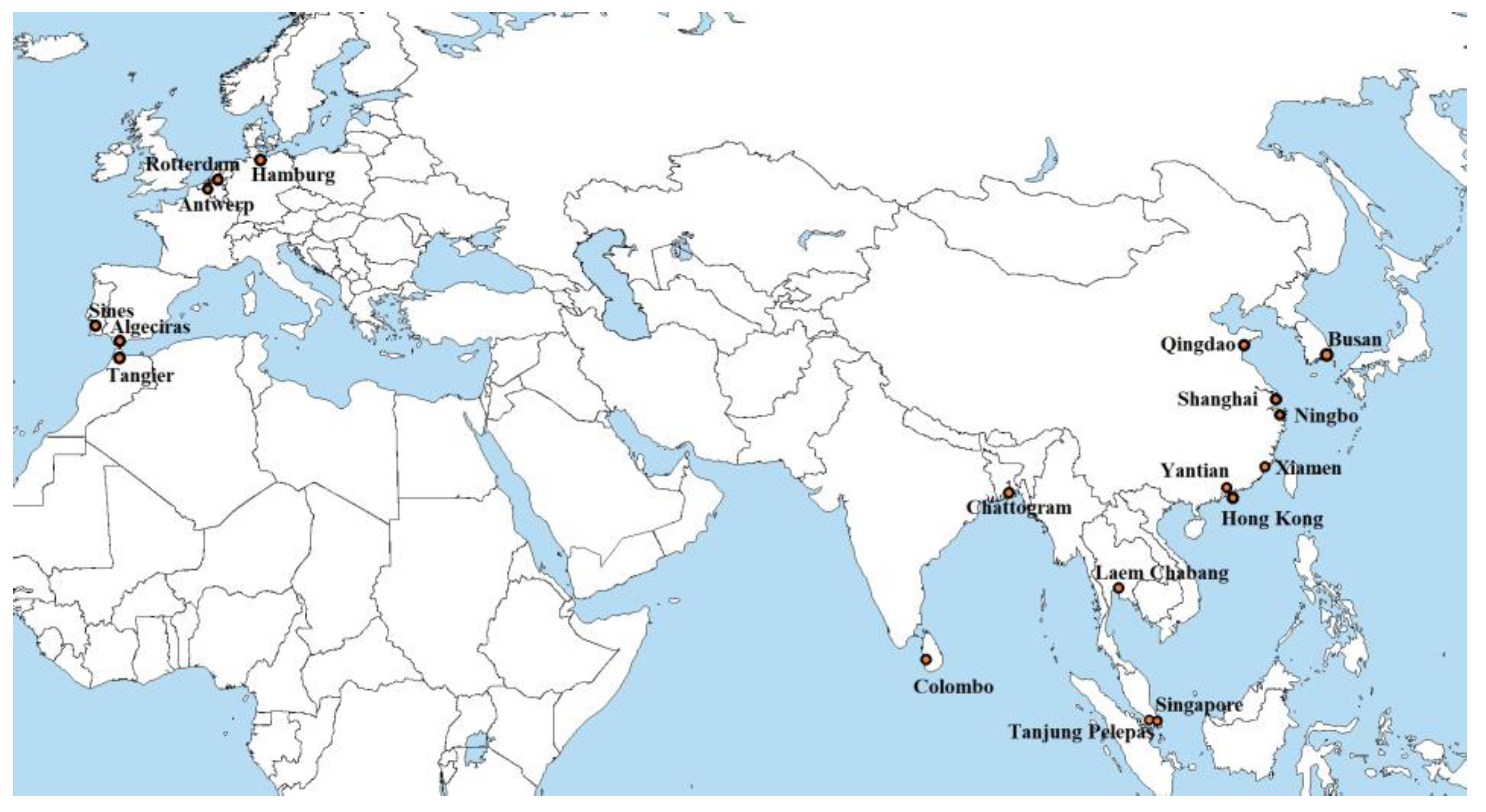
1	Ningbo → Xiamen → Yantian → Tanjung Pelepas → Rotterdam → Port Tanger Med → Hong Kong → Ningbo
2	Shanghai → Yantian → Tanjung Pelepas → Colombo → Port Tanger Med → Hamburg → Antwerp → Port Tanger Med → Singapore → Laem Chabang → Ningbo → Shanghai
3	Antwerp → Rotterdam → Algeciras → Singapore → Hong Kong → Shanghai → Qingdao → Busan → Ningbo → Shanghai→ Yantian → Tanjung Pelepas → Sines → Antwerp
4	Busan → Ningbo → Tanjung Pelepas→ Rotterdam → Tanjung Pelepas → Shanghai → Qingdao → Ningbo → Busan
5	Shanghai → Tanjung Pelepas → Chittagong → Tanjung Pelepas → Singapore → Laem Chabang → Ningbo → Shanghai

, were selected from the Asia–Europe network of a global liner shipping company to evaluate the performance of the proposed model. These routes contain 18 ports, as shown in Figure 4. A total of 250 ships travels on these routes, with 100 ships sailing on each of the first four routes and 50 ships sailing on the last route. The departure time of ships on the five routes is randomly generated from the ranges [1, 75], [1, 80], [1, 90], [1, 85], and [1, 40], respectively. The second numbers in the brackets are the duration required for a ship to complete the corresponding route. The sailing speed is 12 knots, and the planning period is set to five years. The dwell time at each port of call is randomly generated from the range [5, 15]. Having the departure time from the first port of call, the distance between ports of call, ship dwell time, and sailing speed, the set of port–time pairs of each ship can be calculated. The unit fuel cost is USD 110.6/nautical mile according to Meng, Du, and Wang [42] and Wu et al. [43]. The ship cleaning price is randomly generated from [26808, 40549] according to Schultz et al. [44]. The amortized purchasing cost is set to USD 100,000/year. According to Bryers and Characklis [45] and Hakim et al. [2], $\alpha$ and $\beta$ are estimated to be 6.72 and 0.0001, respectively.

5.2. Computational Performance

To test the performance of the solution method, it is compared with an algorithm described in Algorithm 1. This algorithm iteratively solves the upper-level and lower-level problem in sequence until the upper-level solution stays unchanged. A comparison between the proposed solution method and Algorithm 1 is shown in

Table 3. Comparison between the proposed solution method and Algorithm 1.

Planning Period	Computation Time
	Single Level	Algorithm
5	17.1	390.8
10	19.7	430.8
20	20.3	480.5

. Since the planning period will influence total demand, the computation times of the different methods under different planning periods are shown. Results show that transforming the bi-level model to a single level speeds up computation, and the proposed method is therefore suitable for our problem.

Algorithm 1. The heuristic for solving bi-level problems
1	Initialization: Regard all $y_{spt}=1$ in Problem (1), denoted by $y_{spt}^{\ast }$, as the input of P3
2	Repeat until $x_{pn}^{\ast }$ stays unchanged:
3	Solve P3 with $y_{spt}^{\ast }$ and obtain $x_{pn}^{\ast }$
4	Solve P2 with $x_{pn}^{\ast }$ and obtain $y_{spt}^{\ast }$
5	Return $x_{pn}^{\ast }$ and $y_{spt}^{\ast }$

Before solving the bi-level problem, the optimal solution for P1 is first obtained as the input of the bi-level problem. The time consumption is 89.4 s. Every port–time pair with $y_{spt}=1$ is regarded as a cleaning demand. The demand distribution on each port over five years is shown in Figure 5. It shows that the demand is concentrated in only six ports, with only slight variations in demand from year to year at each port.

Having the demand, the bi-level problem can be solved, which takes 17.1 s. The deployment plan of the cleaning equipment is shown in Figure 6. Only four ports are deployed with equipment considering the revenue earned by providing service and the equipment purchase costs. It is worth noting that most of the equipment is purchased in the first year, with a small number of purchases in the second and third year. The reason can be found from Figure 7, which presents the maximal daily demand of the four ports in each year. The maximal demand is roughly the same each year, explaining why procurement is concentrated in the first year. However, there is a slight increase in demand in the second and third year, resulting in additional purchases. The total profit earned for providing cleaning services over the planning period is around USD 45.7 million.

For ships, due to the deployment plan of devices, not all demands can be satisfied. Figure 8 shows a comparison between initial demand and satisfied demand. The lighter bars on the left represent initial demand, while the darker bars on the right represent satisfied demand. Since the Shanghai and Ningbo ports are not equipped with cleaning devices, the demand for these two ports is lost. Similarly, the Singapore and Tanjung Pelepas ports see demand lost due to insufficient equipment supply.

5.3. Sensitivity Analysis

In this section, the impacts of some key parameters are analyzed, such as the demand satisfaction requirements, the cleaning price, and the purchase costs.

It can be seen from the above analysis that some demand is lost due to the lack of cleaning equipment. What if we require all demand be satisfied? The answers are shown in

Table 4. The comparison between partial satisfaction and full satisfaction of demand.

	Revenue (USD, Millions)	Cost (USD, Millions)	Profit (USD, Millions)
Partial satisfaction	153	107	46
Full satisfaction	187	168	19
Change	34	61	−27

. When requiring all demand be satisfied, the service providers can earn USD 34 million more in revenue but spend USD 61 million more on equipment, resulting in a USD 27 million loss in profit. The equipment deployment plan also changes, as shown in Figure 9. The lighter bars on the left represent results without the full demand satisfaction requirement, while the darker bars on the right represent the results of full demand satisfaction. It shows that the ports that previously had no equipment, i.e., Ningbo and Yantian, are now equipped with cleaning devices. The other four ports that previously provided services are now equipped with more equipment, especially in the third year. It suggests that in order for service providers to maintain a loyal customer base, they may need to make a trade-off by sacrificing a portion of their profits.

Second, the impact of cleaning price is explored. The cleaning price in each port is changed in proportion from 0.1 to 10. The influences on demand, equipment deployment, and profits are shown in Figure 9 and elaborated below.

Figure 10a shows total port demand before (referred to as initial demand) and after (referred to as actual demand) the ship is affected by the equipment deployment plan. It shows that when cleaning price is too low, even with very high demand, service providers are reluctant to provide service because the revenue cannot cover the cost. With the increase in cleaning price, the initial demand continues to decline because expensive cleaning costs discourage ships from cleaning for longer periods of time until the additional fouling costs become prohibitively high. As a result, cleaning frequency decreases, which is reflected in the initial demand. The actual satisfied demand follows a broadly similar trend to the initial demand, except for a slight increase when price increases by 2 to 2.5 times. The slight increase can be explained by Figure 10b, which depicts the total demand in each year when the price is 2 and 2.5 times the original price. It is worth noting that when price increases by 2 to 2.5 times, there is only a slight drop in demand. Because the revenue from each demand is increasing, service providers will serve as many demands as possible, so the actual demand will increase slightly. When the price continues to increase because the initial demand is falling, the actual demand is also falling, though the gap between the two will become smaller and smaller.

The total amount of purchased equipment in each year is shown in Figure 10c. When the cleaning price is too low, service providers will not purchase any equipment. When prices continue to increase, equipment purchases generally show a downward trend. However, there is an exception. The reason can be found in Figure 11, which shows the annual equipment deployment of the five ports (because other ports have no equipment deployment). When cleaning price increases, the initial demand may shift between different ports. For example, the ships sailing on route 1 in Table 2 may change their cleaning port from Rotterdam to Ningbo because the rising cleaning price allows ships to sail a longer distance before cleaning. The demand change may result in previously unequipped ports such as Ningbo now having equipment, previously equipped ports such as Rotterdam now without equipment, and changes in deployment between ports.

Overall, increasing cleaning price can increase profits, as shown in Figure 10d. However, in extreme cases when there is no demand, service providers will exit the market.

Finally, the impact of purchase cost was investigated. Purchase cost was changed in proportion from 0.5 to 2.0 with a step size of 0.1, as shown in Figure 12. Figure 12a,b present the variation in equipment deployment plans and total profit. Changing purchase cost does not affect initial demand because purchase cost does not appear in the model of P1, so with the increase in purchase cost the potential revenue stays the same while the cost of equipment increases, resulting in a profit loss and therefore resulting in a reduction in the total amount of purchased equipment. When profit reaches zero, service providers will exit the market, which means no fouling cleaning service can be found in the market.

6. Discussions

There are three main limitations to be acknowledged in this study. Firstly, the assumption that ships that cannot be served will not use the cleaning service on subsequent voyages and will opt for alternative techniques like antifouling painting may have practical implications. Under this assumption, if a ship decides to clean fouling during a port visit but cannot find available cleaning equipment, it will never use the cleaning service again. This means that the service providers lose this customer permanently. This assumption has an impact on the demand for cleaning services, as well as the equipment procurement and deployment decisions made by service providers. If delayed cleaning is allowed, the ship may decide to use the cleaning service at the next port of call, thereby maintaining demand. With increased demand, the revenue of service providers may increase. Future research could consider this aspect and modify the formulation of the model accordingly. Instead of pre-calculating the cleaning demand in P1, the objective function of P1 can become the lower-level objective function. The decision-making process will be constrained by the deployment of cleaning equipment in the upper level, taking into account the possibility of delayed cleaning.

Secondly, the present study assumes that cleaning demands are primarily driven by cost considerations. While cost is an important factor, there are situations where ships are obliged to undergo fouling cleaning irrespective of its cost-effectiveness. For instance, certain countries may enforce regulations mandating the cleaning of fouling before a ship’s entry into their ports. This regulatory requirement significantly influences the demand for cleaning services. To incorporate this realistic situation, future research could introduce a binary parameter for each port that indicates cleaning requirements. If the parameter is set to 1, it signifies that cleaning before the visit is required, otherwise there is no such requirement. This parameter can then be incorporated into the constraints of the lower-level problem to restrict the cleaning decisions accordingly.

Thirdly, this study is based on the assumption that biofouling does not increase while a ship is in motion due to its high speed. However, this assumption may not be universally applicable and can be influenced by various factors, including the specific marine environment, vessel design, and the duration of ship operation. These factors can affect the extent of biofouling settlement during ship motion. To address this limitation and enhance the model’s applicability to a wider range of scenarios, we will consider incorporating fouling accumulation while ships are in motion into the accumulation function in future research. This addition will provide a more comprehensive and accurate representation of biofouling dynamics, accounting for the influence of ship motion on fouling accumulation.

These modifications will address the limitations of the current study and provide a more comprehensive and realistic understanding of the fouling cleaning decision-making process. By considering the possibility of delayed cleaning and incorporating regulatory requirements, research can offer practical insights for decision makers in the industry and enhance the applicability of findings.

7. Conclusions

This research develops a bi-level model to optimize the hull cleaning process. To overcome computational complexity, an efficient approach leveraging the big-M method is employed to convert the problem into a computationally tractable single-level formulation. Comprehensive numerical experiments are conducted to assess the performance of the developed models. The findings highlight several important insights. Firstly, the results indicate that service providers may choose to sacrifice a portion of the demand in order to maximize profits. Additionally, there is a notable concentration of equipment procurement in the initial year due to high demand during that period. Sensitivity analyses are additionally conducted to investigate the impact of key parameters on the system. Notably, the results elucidate that pursuing complete demand satisfaction may yield a substantial USD 27 million loss in profit. Furthermore, manipulating the cleaning price exerts a direct influence on demand levels and equipment purchases, thereby affecting overall profitability. Additionally, variations in purchase costs directly impact profits, resulting in corresponding adjustments to the total number of equipment purchases. Finally, the study reveals that market exit becomes a likely outcome in scenarios where service providers fail to generate profits.

These findings provide valuable insights into optimization of the hull cleaning process and offer practical implications for decision makers in the industry. For service providers, understanding the trade-off between demand satisfaction and profit maximization can help them make strategic decisions on how to best allocate their resources and prioritize their operations. By strategically sacrificing a portion of the demand, service providers can optimize their profitability and resource utilization. Furthermore, the observed concentration of equipment procurement in the initial year due to high demand highlights the need for proactive planning and allocation of resources. Understanding this pattern can assist service providers in effectively managing their equipment inventory and optimizing their procurement strategies to meet the fluctuating demand. Additionally, this study reveals that service providers can directly influence demand levels and equipment purchases by manipulating cleaning prices, thereby affecting their overall profitability. These findings provide valuable guidance for decision makers in formulating pricing strategies to maximize profitability. For ship operators, the insights gained from this study can help them develop cost-effective cleaning strategies. By considering factors such as pricing strategies, equipment procurement patterns, and cost considerations, ship operators can minimize expenses while maintaining the desired level of cleanliness. Importantly, the practical implications of this study extend beyond financial considerations. By optimizing the hull cleaning process, decision makers can significantly reduce the environmental impact associated with marine fouling and improve operational efficiency.

References

- Utama IK, A.P.; Nugroho, B. Biofouling, ship drag, and fuel consumption: A brief overview. J. Ocean Technol. 2018, 13, 42–48. [Google Scholar]
- Hakim, M.L.; Utama, I.K.A.P.; Nugroho, B.; Yusim, A.K.; Baithal, M.S.; Suastika, I.K. Review of correlation between marine fouling and fuel consumption on a ship. In Proceedings of the SENTA: 17th Conference on Marine Technology, Surabaya, Indonesia, 6–7 December 2017; pp. 122–129. [Google Scholar]
- Fitridge, I.; Dempster, T.; Guenther, J.; De Nys, R. The impact and control of biofouling in marine aquaculture: A review. Biofouling 2012, 28, 649–669. [Google Scholar] [CrossRef] [PubMed]
- Farkas, A.; Degiuli, N.; Martić, I.; Vujanović, M. Greenhouse gas emissions reduction potential by using antifouling coatings in a maritime transport industry. J. Clean. Prod. 2021, 295, 126428. [Google Scholar] [CrossRef]
- Dinariyana AA, B.; Deva, P.P.; Ariana, I.; Handani, D.W. Development of model-driven decision support system to schedule underwater hull cleaning. Brodogradnja 2022, 73, 21–37. [Google Scholar] [CrossRef]
- Farkas, A.; Degiuli, N.; Martić, I.; Ančić, I. Energy savings potential of hull cleaning in a shipping industry. J. Clean. Prod. 2022, 374, 134000. [Google Scholar] [CrossRef]
- Yebra, D.M.; Kiil, S.; Dam-Johansen, K. Antifouling technology—Past, present and future steps towards efficient and environmentally friendly antifouling coatings. Prog. Org. Coat. 2004, 50, 75–104. [Google Scholar] [CrossRef]
- Maan, A.M.; Hofman, A.H.; de Vos, W.M.; Kamperman, M. Recent developments and practical feasibility of polymer-based antifouling coatings. Adv. Funct. Mater. 2020, 30, 2000936. [Google Scholar] [CrossRef]
- Evans, L.V. Marine algae and fouling: A review, with particular reference to ship-fouling. Bot. Mar. 1981, 24, 167–171. [Google Scholar] [CrossRef]
- Callow, M. Ship fouling: Problems and solutions. Chem. Ind. 1990, 5, 123–127. [Google Scholar]
- Townsin, R.L. The ship hull fouling penalty. Biofouling 2003, 19 (Suppl. S1), 9–15. [Google Scholar] [CrossRef]
- Monty, J.P.; Dogan, E.; Hanson, R.; Scardino, A.J.; Ganapathisubramani, B.; Hutchins, N. An assessment of the ship drag penalty arising from light calcareous tubeworm fouling. Biofouling 2016, 32, 451–464. [Google Scholar] [CrossRef] [PubMed]
- Demirel, Y.K.; Uzun, D.; Zhang, Y.; Fang, H.C.; Day, A.H.; Turan, O. Effect of barnacle fouling on ship resistance and powering. Biofouling 2017, 33, 819–834. [Google Scholar] [CrossRef] [PubMed]
- Coraddu, A.; Oneto, L.; Baldi, F.; Cipollini, F.; Atlar, M.; Savio, S. Data-driven ship digital twin for estimating the speed loss caused by the marine fouling. Ocean Eng. 2019, 186, 106063. [Google Scholar] [CrossRef]
- Demirel, Y.K.; Song, S.; Turan, O.; Incecik, A. Practical added resistance diagrams to predict fouling impact on ship performance. Ocean Eng. 2019, 186, 106112. [Google Scholar] [CrossRef]
- Farkas, A.; Degiuli, N.; Martić, I.; Dejhalla, R. Impact of hard fouling on the ship performance of different ship forms. J. Mar. Sci. Eng. 2020, 8, 748. [Google Scholar] [CrossRef]
- Song, S.; Demirel, Y.K.; Muscat-Fenech CD, M.; Tezdogan, T.; Atlar, M. Fouling effect on the resistance of different ship types. Ocean Eng. 2020, 216, 107736. [Google Scholar] [CrossRef]
- Farkas, A.; Degiuli, N.; Martić, I. An investigation into the effect of hard fouling on the ship resistance using CFD. Appl. Ocean Res. 2020, 100, 102205. [Google Scholar] [CrossRef]
- Erol, E.; Cansoy, C.E.; Aybar, O.Ö. Assessment of the impact of fouling on vessel energy efficiency by analyzing ship automation data. Appl. Ocean Res. 2020, 105, 102418. [Google Scholar] [CrossRef]
- Tribou, M.; Swain, G. Grooming using rotating brushes as a proactive method to control ship hull fouling. Biofouling 2015, 31, 309–319. [Google Scholar] [CrossRef]
- Oliveira, D.R.; Granhag, L. Ship hull in-water cleaning and its effects on fouling-control coatings. Biofouling 2020, 36, 332–350. [Google Scholar] [CrossRef]
- Zhong, X.; Dong, J.; Liu, M.; Meng, R.; Li, S.; Pan, X. Experimental study on ship fouling cleaning by ultrasonic-enhanced submerged cavitation jet: A preliminary study. Ocean Eng. 2022, 258, 111844. [Google Scholar] [CrossRef]
- Farkas, A.; Degiuli, N.; Martić, I. The impact of biofouling on the propeller performance. Ocean Eng. 2021, 219, 108376. [Google Scholar] [CrossRef]
- Farkas, A.; Degiuli, N.; Martić, I. Assessment of the effect of biofilm on the ship hydrodynamic performance by performance prediction method. Int. J. Nav. Archit. Ocean Eng. 2021, 13, 102–114. [Google Scholar] [CrossRef]
- Georgiev, P.; Garbatov, Y. Multipurpose vessel fleet for short black sea shipping through multimodal transport corridors. Brodogradnja 2021, 72, 79–101. [Google Scholar] [CrossRef]
- Degiuli, N.; Farkas, A.; Martić, I.; Grlj, C.G. Optimization of maintenance schedule for containerships sailing in the Adriatic Sea. J. Mar. Sci. Eng. 2023, 11, 201. [Google Scholar] [CrossRef]
- Chang, J.S.; Mackett, R.L. A bi-level model of the relationship between transport and residential location. Transp. Res. Part B Methodol. 2006, 40, 123–146. [Google Scholar] [CrossRef]
- Stoilova, K.; Stoilov, T. Model predictive traffic control by bi-level optimization. Appl. Sci. 2022, 12, 4147. [Google Scholar] [CrossRef]
- Gang, J.; Tu, Y.; Lev, B.; Xu, J.; Shen, W.; Yao, L. A multi-objective bi-level location planning problem for stone industrial parks. Comput. Oper. Res. 2015, 56, 8–21. [Google Scholar] [CrossRef]
- Abareshi, M.; Zaferanieh, M. A bi-level capacitated P-median facility location problem with the most likely allocation solution. Transp. Res. Part B Methodol. 2019, 123, 1–20. [Google Scholar] [CrossRef]
- Casas-Ramírez, M.S.; Camacho-Vallejo, J.F.; Díaz, J.A.; Luna, D.E. A bi-level maximal covering location problem. Oper. Res. 2020, 20, 827–855. [Google Scholar] [CrossRef]
- Camacho-Vallejo, J.F.; González-Rodríguez, E.; Almaguer, F.J.; González-Ramírez, R.G. A bi-level optimization model for aid distribution after the occurrence of a disaster. J. Clean. Prod. 2015, 105, 134–145. [Google Scholar] [CrossRef]
- Lee, M.C.; Wee, H.M.; Wu, S.; Wang, C.E.; Chung, R.L. A bi-level inventory replenishment strategy using clustering genetic algorithm. Eur. J. Ind. Eng. 2015, 9, 774–793. [Google Scholar] [CrossRef]
- Qi, J.; Wang, S.; Psaraftis, H. Bi-level optimization model applications in managing air emissions from ships: A review. Commun. Transp. Res. 2021, 1, 100020. [Google Scholar] [CrossRef]
- Wang, K.; Li, J.; Yan, X.; Huang, L.; Jiang, X.; Yuan, Y.; Negenborn, R.R. A novel bi-level distributed dynamic optimization method of ship fleets energy consumption. Ocean Eng. 2020, 197, 106802. [Google Scholar] [CrossRef]
- Zhu, M.; Shen, S.; Shi, W. Carbon emission allowance allocation based on a bi-level multi-objective model in maritime shipping. Ocean Coast. Manag. 2023, 241, 106665. [Google Scholar] [CrossRef]
- Yang, D.; Pan, K.; Wang, S. On service network improvement for shipping lines under the one belt one road initiative of China. Transp. Res. Part E Logist. Transp. Rev. 2018, 117, 82–95. [Google Scholar] [CrossRef]
- Zhuge, D.; Wang, S.; Zhen, L.; Laporte, G. Subsidy design in a vessel speed reduction incentive program under government policies. Nav. Res. Logist. 2021, 68, 344–358. [Google Scholar] [CrossRef]
- Ziar, E.; Seifbarghy, M.; Bashiri, M.; Tjahjono, B. An efficient environmentally friendly transportation network design via dry ports: A bi-level programming approach. Ann. Oper. Res. 2023, 322, 1143–1166. [Google Scholar] [CrossRef]
- Wang, W.; Wang, S.; Zhen, L. Optimal subsidy design for energy generation in ship berthing. Marit. Policy Manag. 2023, 1–14. [Google Scholar] [CrossRef]
- Cai, L.; Wu, Y.; Zhu, S.; Tan, Z.; Yi, W. Bi-level programming enabled design of an intelligent maritime search and rescue system. Adv. Eng. Inform. 2020, 46, 101194. [Google Scholar] [CrossRef]
- Meng, Q.; Du, Y.; Wang, Y. Shipping log data based container ship fuel efficiency modeling. Transp. Res. Part B Methodol. 2016, 83, 207–229. [Google Scholar] [CrossRef]
- Wu, Y.; Huang, Y.; Wang, H.; Zhen, L. Nonlinear programming for fleet deployment, voyage planning and speed optimization in sustainable liner shipping. Electron. Res. Arch. 2023, 31, 147–168. [Google Scholar] [CrossRef]
- Schultz, M.P.; Bendick, J.A.; Holm, E.R.; Hertel, W.M. Economic impact of biofouling on a naval surface ship. Biofouling 2011, 27, 87–98. [Google Scholar] [CrossRef]
- Bryers, J.; Characklis, W. Early fouling biofilm formation in a turbulent flow system: Overall kinetics. Water Res. 1981, 15, 483–491. [Google Scholar] [CrossRef]