Hydrodynamic Simulation of Green Hydrogen Catamaran Operating in Lisbon, Portugal

Abstract

Similar to other industries, the maritime industry is also facing increasing restrictions on ships regarding pollution control. The research presented in this paper is aimed at studying the pros and cons of alternative fuels followed by a detailed analysis on hydrogen fuel cells (PEMFC) for a particular ship operating in Lisbon, Portugal. Dynamic forces acting on the ship have been studied for a year. Assessing various scenarios based on these results aids ship operators in making informed decisions regarding the future course of action for their existing vessels. These different cases are first: business as usual (diesel engine), second: replacing the diesel engine with a hydrogen hybrid system and, third: replacement of the ship with a new hydrogen hybrid ship. The study is based on the simulation of numerical equations and CFD simulation results. As the result, the second scenario is best suited in both aspects; namely, environmental and economic.

1. Introduction

It is estimated that around 80–90% of international trade is facilitated by maritime vessels, which is largely attributed to its cost efficiency in transportation [1]. There is a direct relationship between world trade and world economic growth [2,3]. Therefore, with the increasing world economy and shipping industry, carbon emissions are also expected to swell if business continues as usual. To address this challenge, the International Maritime Organization (IMO) has made several efforts to control these emissions by formulating emissions related to policies and regulations. There are a range of measures that an operator can adopt to achieve these reductions like regulatory requirements (energy efficiency design index, ship energy efficiency management plan, etc.), advancements in technology (improved engines, alternative fuels, etc.), adjustments related to a ship’s operation (slow steaming, low emission fuels, etc.), and market-based instruments (cap-and-trade systems, rebate mechanism, etc.) [4]. On top of the IMO’s regulations, local governments are also actively taking part in policy making. The recent example of such a policy is an agreement related to emission trading systems (EU ETS) made by the EU’s legislative bodies in January 2023, and to be enforced in January 2024, which penalizes the ship operators based on the amount of carbon emitted.

It is evident that shipping significantly impacts both the economy and the environment. Therefore, it is important to study available options to reduce the environmental impact while the shipping industry keeps booming. Pros and cons of available alternative fuels are studied to boil down to only one which is than studied on the selected ship. A SIMULINK model is designed for the catamaran ferry “Almadense” (the selected ship) operating on Tagus River. The following objectives are studied:

• To study an alternative fuel technology (the hydrogen fuel cell) for the ship considered in this study.
• To develop a MATLAB SIMULINK model of a power system and subsequently reproduce year-long simulation outcomes by utilizing year-long data inputs.
• To perform lifetime economic and environmental analyses for all the three considered cases.
• To suggest the optimum size of hybrid system components.

2. Literature Review

Carbon emissions contribution via shipping increased from 1.8% in 1996 to 2.9% in 2018 [5,6]. Numerous studies have been conducted to evaluate the potential application of different technologies across a spectrum of ship sizes and travel routes. The economic factor proved to be the most influencing factor for the implementation of potential technologies [5]. Another key parameter for the selection of new technology is the required power and distance for travel. This is due to the size and storage restrictions along with efficiencies, route predictability, present technology capabilities, and up-front costs [7].

Although very low sulphur fuel oil (VLSFO) is currently in use, because of new IMO regulation enforcements that went into effect in 2020, there are a variety of alternate fuels such as liquefied natural gas (LNG), methanol, liquid petroleum gas (LPG), ethanol, hydrogen, etc., that have better GHG emission reduction potentials. Amongst these, currently LNG is the most studied alternative fuel. On the other hand, green hydrogen provides a cleaner and efficient fuel, but it is limited to short-range shipping [5]; these fuels have been compared with conventional marine gas oils (MGO) in terms of their physical parameters [8], as shown in

Table 1. Properties of different fuels that could be used as alternative fuels for power generation [8].

Parameter	Density	LHV	Vol. Energy Density	Volume
	[t/m3]	[GJ/t]	[GJ/m3]	[m3/GJ; Normalized]
MGO	0.835	42.7	35.7	1
LPG	0.49	46	22.6	1.58
H2 @350 bar	0.023	120	2.8	12.78
H2 liquid	0.071	120	8.52	4.18
Ammonia	0.61	18.6	11.4	3.17

. These parameters are especially important when considering their storage requirements.

In terms of transportation, liquid or gaseous hydrogen transportation is more efficient compared to ammonia [9].

A hybrid combination of hydrogen and green ammonia is suggested in [10] for the best environmental performance whereas dual fuel engine with LNG is considered to have the best net present value (NPV) performance. These calculations also include carbon taxes, which are not applicable for the case study presented in this paper. Ammonia is also toxic for humans and it could incur a negative NPV due to its high operation costs [10,11].

For short-distance transits of small- to medium-sized ships, compressed hydrogen emerged as the dominant choice [12]. In a hybrid system, fuel cells (FCs) have a higher energy density with a considerably lower power density, whereas batteries exhibit a higher power density, which complements the characteristics of FCs (as shown in Figure 1), summing up to make a hybrid system.

Electrochemical energy is harvested and converted into electrical energy in a hydrogen FC. Fundamentally, there are different types of FC technologies available today, amongst which the PEMFC (proton exchange membrane fuel cell) is the best suited for ships with lower power demands like ferries, boats, and fishing vessels. The PEMFC is amongst the lightest and most compact FC with high power density and efficiency. Additionally, PEMFCs have a higher cold start potential with better transient performance [13].

Figure 1. Ragone plot adapted from [14] for various types of emerging green technologies to power the energy system based on their power and energy densities.

Figure 1. Ragone plot adapted from [14] for various types of emerging green technologies to power the energy system based on their power and energy densities.

The study presented in [15] ranks FC technologies on different parameters; namely, safety, emissions, efficiency, cost, lifetime, power output, fuel type, and size on a scale of five. The Molthen Carbonate Fuel Cell (MCFC) operating on diesel oil (diesel oil undergo reforming process to extract hydrogen) scores the highest, although it is not an environment friendly alternative. The PEMFC scores the second highest.

A robust and fairly accurate numerical simulation of the PEMFC was performed by [16] on a marine vessel. The study concentrated on assessing the dynamic response of fuel cells within a hybrid system subjected to step load changes. This highlights the possibility of achieving a good fidelity using dynamic simulations. Another study [17] quantified the emission reduction of a ferry in Denmark that used a hybrid hydrogen system; the authors determined a total decline of 65% in greenhouse gases. This massive reduction highlights the potential of such technology in achieving the desired goal of emissions reduction. But this reduction in emission comes with an increased economic cost. The adoption of the PEMFC as the primary power source for marine ships results in a heightened cost, ranging between 35% and 38% higher than conventional diesel propulsion and with this price surge, a notable reduction of 73–78% in GHGs emissions can be achieved [18].

Further insights into this decline have been examined in reference [19], where a liquified natural gas fuel cell (LNGFC) demonstrated a superior performance compared to a PEMFC. However, LNGFCs comes with a cost that is nearly three times the price of PEMFCs. AFC, SOFC, and low-temperature PEMFCs exhibit efficiencies in the range of 50% to 60%, surpassing all the other FCs. Quantitatively, a low-temperature PEMFC consumes the least hydrogen fuel (approximately 60 g/kWh) [19]. Apart from all these advantages of PEMFCs over other FC types, PEMFCs are easily available in the market and have extended maintenance intervals [19], making it a better choice overall. These are potential figures and need to be verified in actual scenarios. There are 3123 ferries which are equipped with FCs onboard [18], some of which only utilize FCs for auxiliary power demands. This suggests that the implementation of FCs in the marine sector is still in the R&D phase [20]. Therefore, a significant economic investment along with technological development is required.

Identified Research Gaps

• There is a lack of studies that simulate the model under real environmental conditions. Most of the studies were performed while assuming the average condition of a voyage using simplified numerical methods.
• There are no studies, to the best of the authors’ knowledge, that analyzes the lifetime economic cost of running the ship (with new technology) and the environmental emissions for an already commissioned ship under different possible scenarios. Such an analysis would consider the scenario of the ship’s continuous operation on diesel for its remaining lifespan, or with a transition to alternate technology, or through decommissioning and replacement with a new alternate fuel-powered ship.
• According to the literature review, it is clear that a unique analysis of the selected technology for a particular ship on a specified route is required.
• There is a lack of studies that calculate the power system component sizing based on the real environmental condition simulation that balances both economic and environmental concerns.

3. Methodology

This study focuses on the analysis of the catamaran ferry “Almadense”, currently in operational service in Lisbon whose specifications are as per

Table 2. Specifications of the catamaran ferry “Almadense”, operating on the route Porto Brandão, Belém, and Trafaria in Lisbon, Portugal [21].

	Value	Unit
Capacity	360 + 29	PAX + Vehicle
Length	47.5	m
Beam	16	m
Depth	3.65	m
Draft	2.2	m
Gross Tonnage	1479	t

. Operating along the River Tagus, this diesel-powered catamaran connects three key ports: Porto Brandão, Belém, and Trafaria, as illustrated in Figure 2. The vessel boasts a catamaran-style hull design renowned for its high efficiency, primarily attributed to minimized hull drag forces.

The ship starts its operation in the morning at 05:30 a.m. and the last voyage finishes at 09:30 p.m. when it arrives at Porto Brandão, concluding a daily voyage composed of 55 trips. The block coefficient “$C_B$” of the ship has been calculated numerically using Equation (1) where $Fn$ is the Froude number. This $C_B$ is essential to calculating the hydrodynamic forces (wave and hull resistance). There are many ways of estimating it; one that has been used in this study includes Fn (Froude number) according to [22]. The study limited the range of Fn between 0.27 and 0.36 for passenger ships [22]. This range is used as a verification method to verify the $C_B$. The ship considered in this study satisfies this range with Fn of 0.28. This acts as additional yet simpler approach for $C_B$ verification:

$$C_B=1.2-2.378Fn$$

(1)

3.1. Case I—Hydrogen Hybrid System Modelling

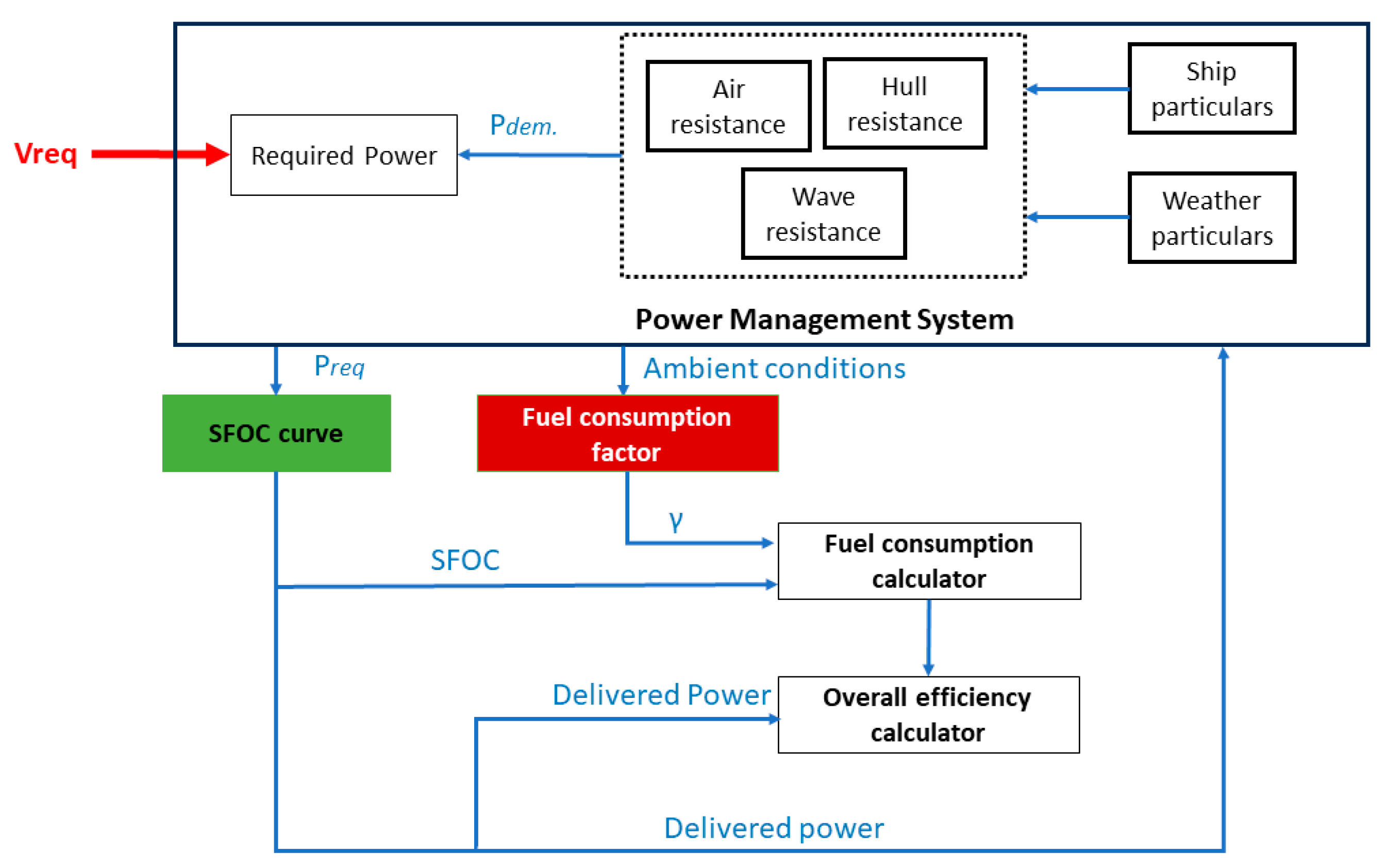
To have an optimal design of an energy system, a hybrid power system is designed in MATLAB SIMULINK with the principle as shown in Figure 3. The design simply works on the principle that in order to propel the ship at a certain advance speed, it has to overcome all the resistance that it would encounter which includes hull, waves, and air resistances. If the power supplied overcomes these resistances, the ship will start moving at the desired speed.

The speed profile of the ship for an average day is used as an input to simulate the designed model. The velocity demand profile is kept constant (as shown in Figure 4), but environmental conditions of the ship’s operation vary. This variation changes the power demand even for the same velocity demand.

The power needed by the ship is influenced by various external forces as previously mentioned. An outlined representation of the power required is depicted in Figure 5, incorporating factors such as the instantaneous wave height (ξ_wave), water-specific weight (σ_wave), wind speed (v_air), actual wind direction (θ_air), air pressure (P_air), air density (ρ_air), resulting ship speed (v_ship), and direction (θ_ship). To provide this power demand, a modular FC with a unit capacity of 200 kW inspired by Ballard’s FcWave module [23] is used in this study. The characteristic and efficiency curves of this FC are assumed as shown in Figure 6 and Figure 7, respectively.

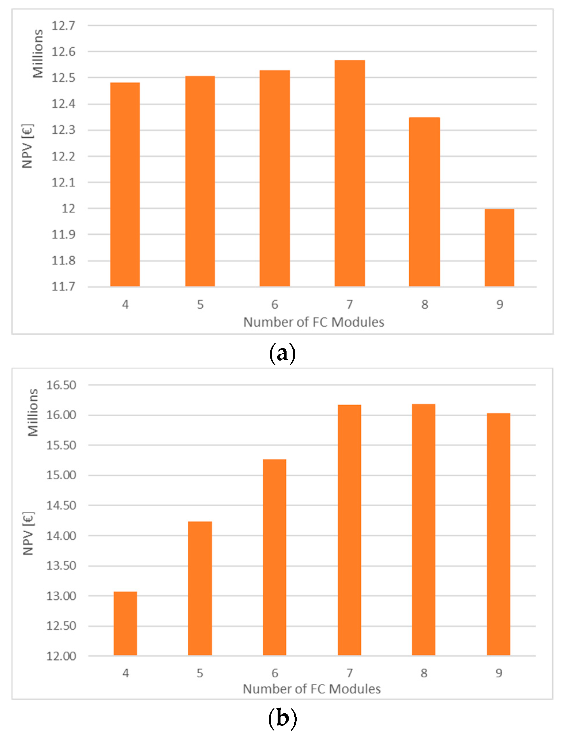
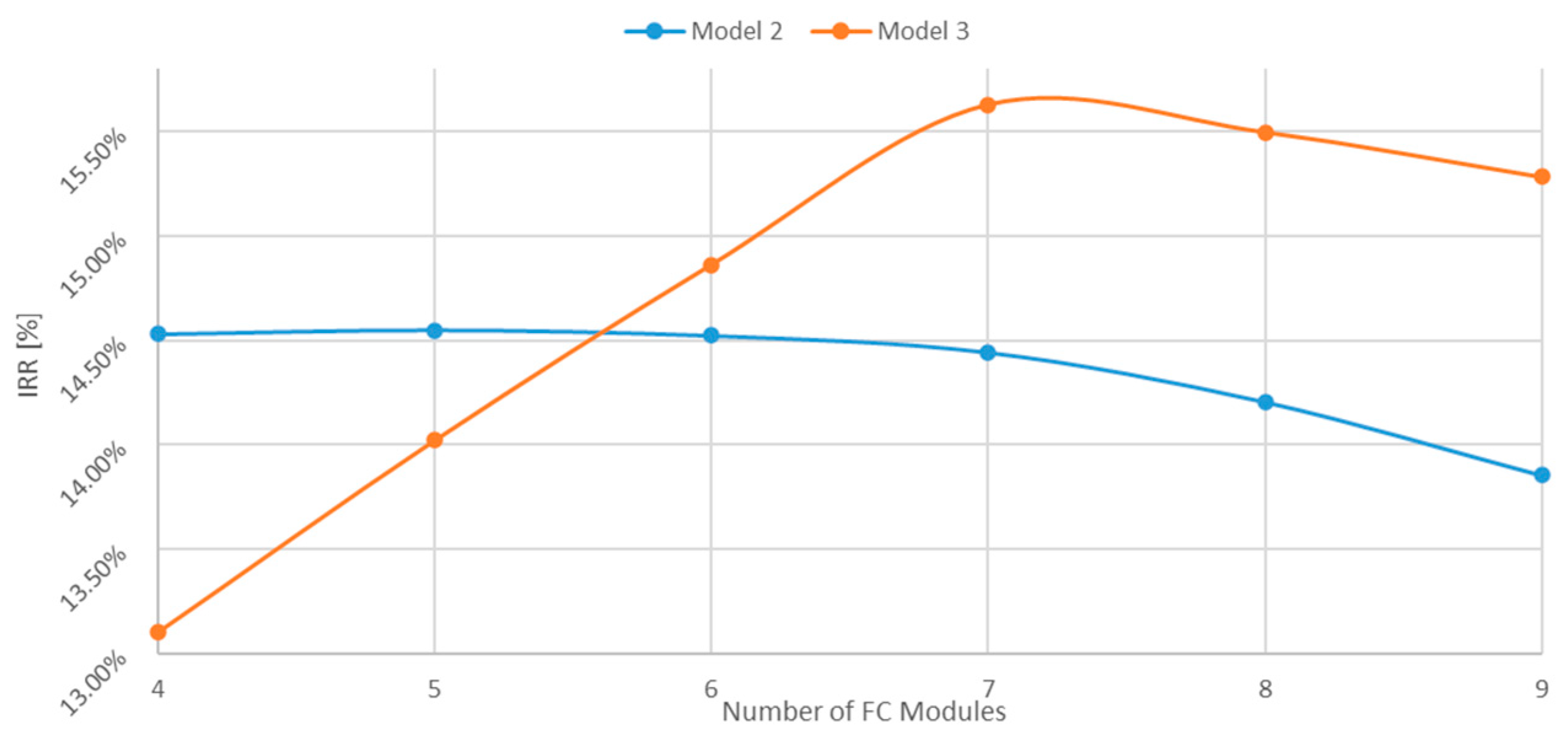
The FC module generates varying voltage and current outputs, necessitating the use of a DC–DC boost converter to maintain a constant voltage for the propulsion motor. Multiple simulations were conducted, altering the number of FC modules to determine the optimal module numbers. A crucial determining factor is the annual hydrogen consumption, directly influencing the operating expense (OPEX). To calculate the hydrogen used, the hydrogen mass flow is required, which is calculated during the simulation for every simulation step using Equation (2):

$${\dot{m}}_{H_2}=\frac{{P_{fc}}^{*}}{{\mathsf{\eta }}_{fc}\widehat{{LHV}_{H_2}}}$$

(2)

where ${P_{fc}}^{*}$ is the power delivered by the FC, ${\mathsf{\eta }}_{fc}$ is the FC efficiency for the corresponding load, and $\widehat{{LHV}_{H_2}}$ is the lower heating value of hydrogen. The DC–DC boost converter stabilizes the voltage output to 815 V corresponding to the voltage requirements of the DC propulsion motor (because of high torque). The motor used here is an ABB DC motor with Cat. No. 3BSM003050-XVJ with a power rating of 1355 kW at 970 rpm.

Apart from the power requirement of the propulsion, the power system in this study is also designed to supply energy to the ship’s auxiliary demands. The auxiliary system includes all the necessary equipment like communication, navigation, fire management systems, etc., along with all the devices required for comfortable movements of crew and passengers like air conditioning system, lighting, power ramps, etc. This study assumes that this power is fixed at a constant value of 50 kW. The power supplied while in port is sourced from a battery power pack. In the designed hybrid power system, if the number of FC modules is less (while using a simulation to track different module numbers) but there is a higher power demand exceeding FC capacity, the battery pack supplements the FC system for propulsion. This leads to an increase in the battery size to accommodate the combined power needs. Apart from this, the battery also provides interim power until the FC catches up. Equation (3) represents the total power available in the bus bar where $I_{BATTERY}$ and $I_{BFC}$ are currently drawn from the battery and the fuel cell modules, respectively, and $V$ is the bus bar voltage:

$${(I}_{FC}+I_{BATTERY})V=P_M$$

(3)

3.1.1. Power Management System (PMS)

The PMS evaluates real-time conditions acting on the vessel, and their effects are compared with required power, i.e., the desired speed. After evaluation, as a result, its output is the net required power for the ferry to continue to propel at the set speed, which instructs the energy producers either to increase or decrease the power. This is accomplished in simultaneous stages by performing simultaneous calculations. The PMS calculates the difference between the delivered power and the power opposing the propulsion ship due to environmental forces (namely, wave and wind forces and air resistance).

The PMS senses the difference in power and guides the energy providers either to increase or decrease power delivery. These decisions are defined as per Equations (4)–(7):

$$P_{error}\left(t\right)=P_{ef}\left(t\right)-P_{del}\left(t\right)$$

(4)

$${P_{req}}^{*}\left(t\right)=K_p{P}_{error}\left(t\right)+K_i\int P_{error}\left(t\right)+K_d\frac{∆P_{error}\left(t\right)}{∆t}$$

(5)

$$P_{ef}\left(t\right)=\left(F_{wave}\left(t\right)+F_{air}\left(t\right)+F_{hull}\left(t\right)\right)v\left(t\right)$$

(6)

$${P_{req}\left(t\right)}^{}={P_{req}}^{*}\left(t\right)+P_{aux}\left\{\begin{array}{c}{0\le P^{*}}_{req}\left(t\right)-P_{aux};and\\ {P^{*}}_{req}\left(t\right)-P_{aux}\le {\mathit{P}}_{\underset{\mathit{motor}}{\max }}\end{array}\right.$$

(7)

where $P_{error}\left(t\right)$ is the generated difference, $P_{ef}\left(t\right)$ is the total power opposing the propulsion, $P_{del}\left(t\right)$ is the power delivered by the propulsion motor, ${P_{req}}^{*}\left(t\right)$ is the power requirement except for auxiliary power, and $K_p,K_d,\mathrm{a}\mathrm{n}\mathrm{d}{K}_i$ are the controller constants which are obtained after repeated trials of many combinations. 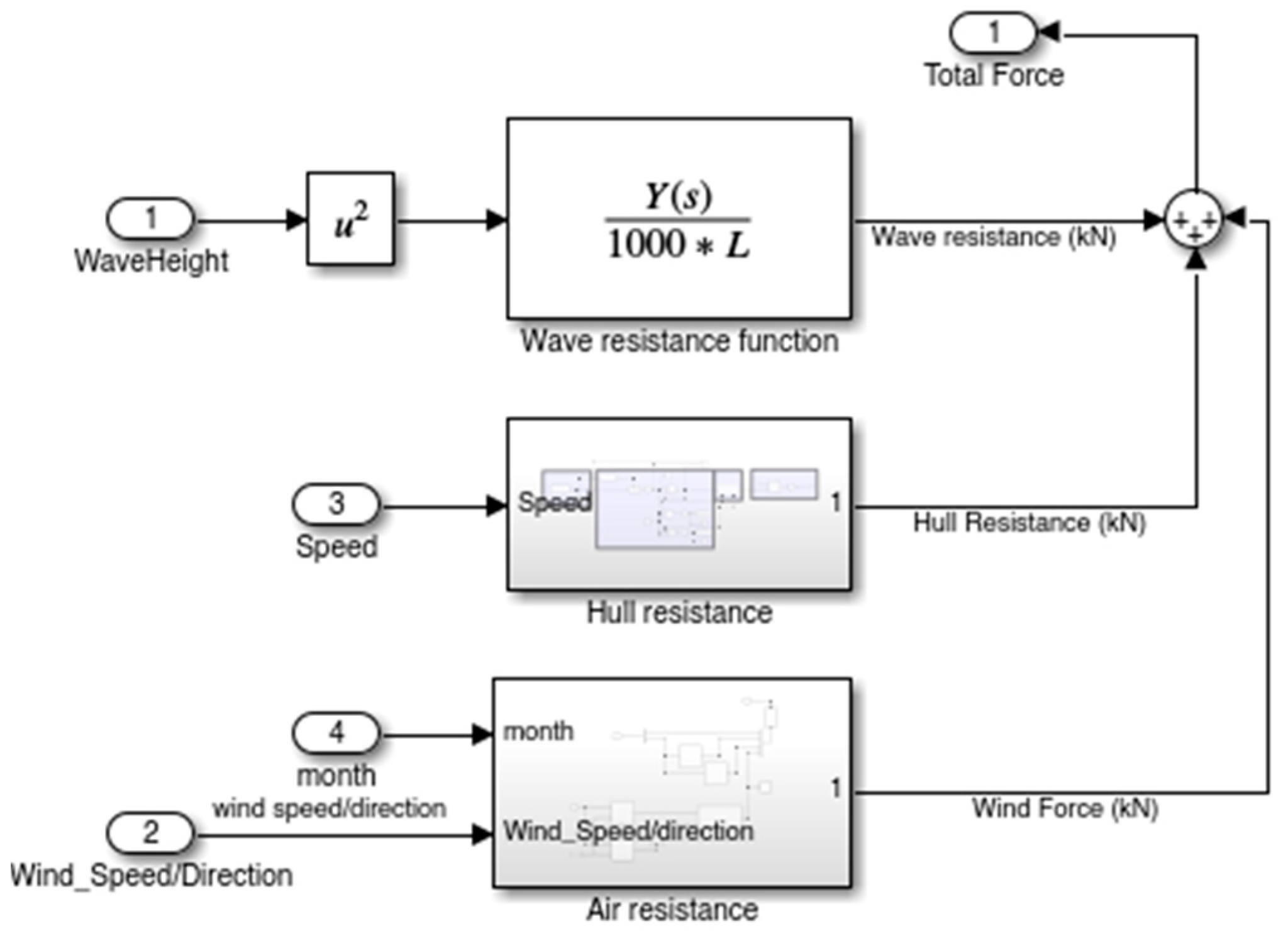Lastly, $F_{wave}\left(t\right),F_{air}\left(t\right),\mathrm{a}\mathrm{n}\mathrm{d}{F}_{hull}\left(t\right)$ are the external environment forces. The total forces are calculated in SIMULINK as shown in Figure 8; $P_{req}\left(t\right)$ is the total required power estimated by the PMS and $v\left(t\right)$ is the ship’s surge velocity. The power is limited by maximum motor power ($P_{\underset{motor}{\mathrm{m}\mathrm{a}\mathrm{x}}}$). Here, ${P_{req}}^{*}\left(t\right)$ is estimated by using a PID controller. This controller varies the amount of hydrogen and oxygen (or battery power in the case of battery operation) using the standard PID Equation (5). Auxiliary power demand is added to this, making the total demand power ${P_{req}\left(t\right)}^{}$, whereas the opposing forces demands $P_{ef}\left(t\right)$. Fundamentally, this $P_{ef}\left(t\right)$ has to be satisfied. After all the system losses, $P_{del}\left(t\right)$ is the power that has been delivered by the propeller which has to satisfy $P_{ef}\left(t\right)$ need. If there is a mismatch, $P_{error}\left(t\right)$ appears, resulting in an increase or decrease in ${P_{req}}^{*}\left(t\right)$. This process of repetitive iterations will continue until $P_{error}\left(t\right)$ reaches zero (or to a minimum error limit).

The wave resistance is calculated via Equation (8) [24]. The wave height (ξ(t)) in this equation is dynamic and is different for every month.

$$∆F_{wave}=\raisebox{1ex}{$0.64{\xi \left(t\right)}^2{B}^2{C}_B\sigma $}\!\left/ \!\raisebox{-1ex}{$L$}\right.$$

(8)

Here, σ is the specific weight of water, L is the length of the ship, and B corresponds to the breadth of the ship. For the simulation performed in this study, the average of each month is used for every second of the ship’s operational day. Similarly, the air resistance is governed via Equation (9) where the density of air varies each month of the year. This density depends on ambient temperature and pressure conditions:

$$F_{air}=\frac{1}{2}{C}_d{\rho }_{air}{A}_{proj.}{v^2}_{attack}$$

(9)

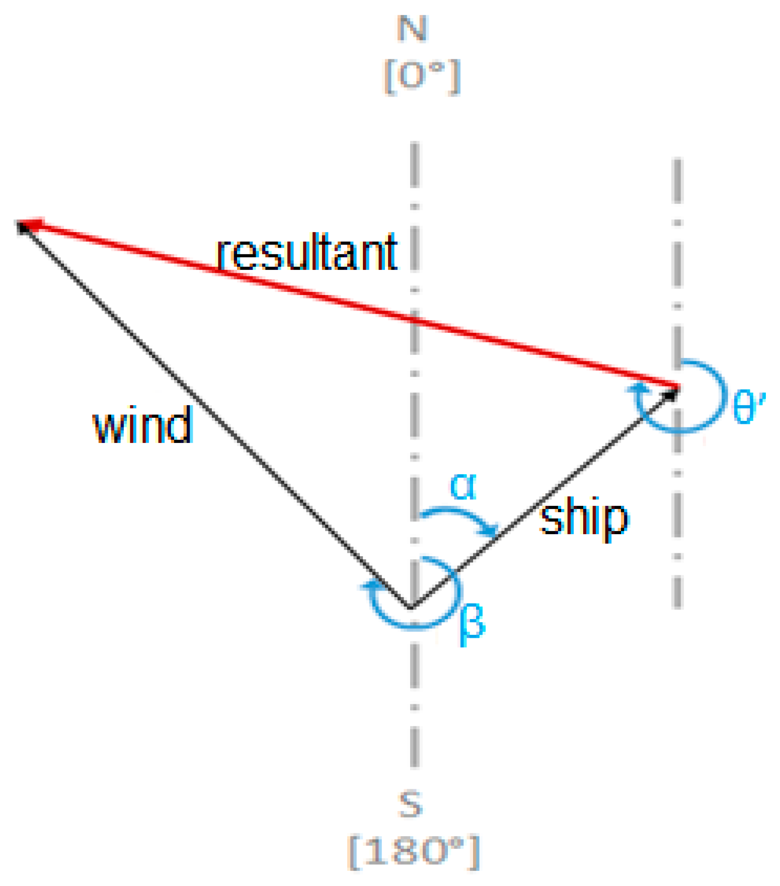
where $C_d$ is the drag coefficient of the ship that depends on the angle of attack of the incoming wind; ${\rho }_{air}$ is the density of air; $A_{proj.}$ is the projected sectional area of the ship for incoming wind that depends on the angle of the incoming wind. Lastly, $v_{attack}$ is the resultant velocity of incoming wind. This velocity is relative to the actual wind speed and direction in addition to the ship’s speed and direction. This resultant wind velocity and direction is calculated as a vector product of both the velocities as represented in Figure 9.

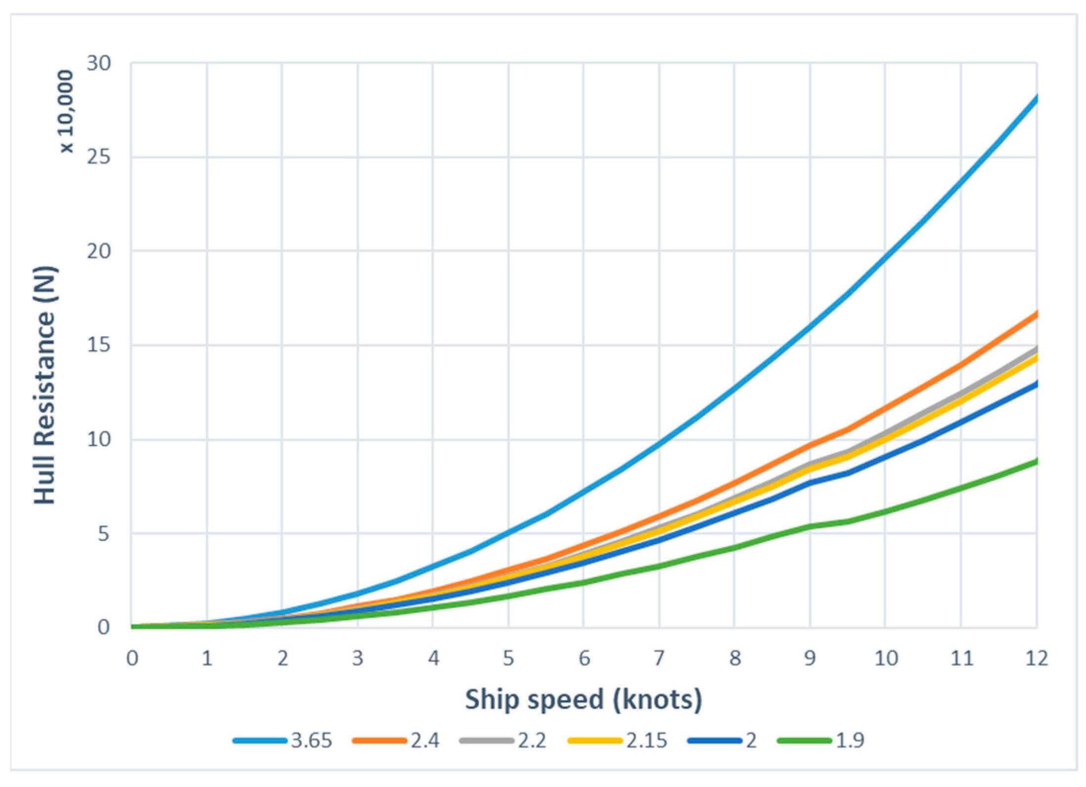
Lastly, the hull force (the force exerted by water) is calculated in the simulation. This force depends on the draft of the ship as the higher the draft, the higher the hull force. Therefore, this force is simulated by varying the draft using a randomizer block of the SIMULINK library depicting change in the ship’s draft (passenger + cars). This randomizer block generates a random signal for each voyage that changes the number of passengers and vehicles transported. The number of passengers and vehicles changes the displacement of the ship and hence affects the draft according to Equations (10) and (11). A CFD analysis of the designed model satisfying the physical parameters was conducted using the CFD simulation ANSYS Fluent software [25] to calculate the force exerted by moving water at various drafts. The results are input into the SIMULINK model as a 2D lookup table (see Figure 10). During the simulations, this 2D lookup table provides the force corresponding to the calculated draft.

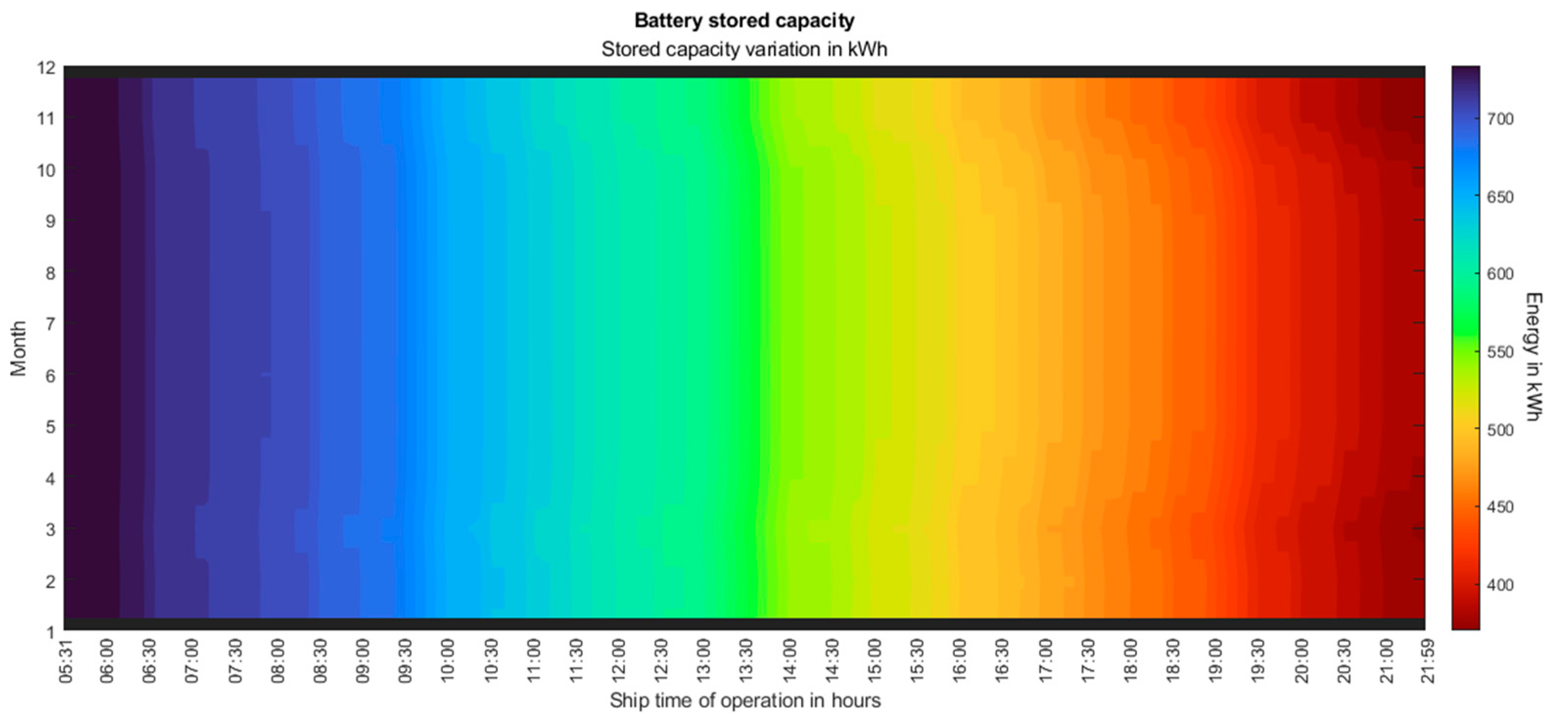
$$T=T_{lightweight}+T_{added}$$

(10)

$${T^{\prime }}_{added}=\frac{W_{added}}{1000TPC}\left[cm\right]$$

(11)

Here, T is the calculated draft, $T_{lightweight}$ is the light weight draft of the ship, $T_{added}$ is the draft added due to the added weight in meters, ${T^{\prime }}_{added}$ is the added draft in centimeters, $W_{added}$ is the total weight added, and $TPC$ is the parameter of the ship that represents the weight needed to change the draft by 1 cm. The study involves the meticulous consideration of monthly data, wherein environmental parameters were meticulously recorded every second throughout the ship’s operational duration. The process involved calculating the average environmental parameters for each specific time instance (e.g., 6:31 a.m.) across the entire month. This method was consistently applied across various months within the year, enabling the representation of average environmental parameters for each month.

The sum of all these forces results in the total force, and consequently the product of this total force and the actual velocity of the ship provides the opposing power $P_{ef}\left(t\right)$.

3.1.2. Energy Management System (EMS)

The EMS is responsible for the decision to distribute the power requirement between both the energy providers (FCs and the battery system). To accomplish that, firstly the system must check if the vessel is in port or sailing since the FC system is not designed in this study to operate in port and switch to ideal conditions (air purging). The EMS is responsible for deciding the energy distribution as shown in the decision flow diagram Figure 11. The FC capacity depends on the number of modules that change for each simulation.

3.2. Case II—Diesel Engine Modelling

It is important to compare the hybrid system with a conventional diesel engine-powered system (current system) in order to produce a holistic analysis. To perform this analysis, the diesel engine system is also modelled in SIMULINK and simulated under exactly the same conditions. In this study, a MAN Diesel & Turbo 8L23/30A 4-stroke IMO Tier II engine [26] is considered with a power rating of 1280 kW. Also, as there is only one energy provider (a diesel engine), the EMS is omitted. The only variables left to calculate are the efficiency and the fuel consumption. For fuel consumption calculations, the specific fuel oil consumption (SFOC) outlined under the reference conditions has been employed, resulting in the tabulated consumptions presented in

Table 3. MAN 8L23/30A SFOC consumption at different engine loads.

Load [%]	100	85	75	50	25
SFOC [g/kWh]	194	193	192	194	210

:

But in actual conditions, the SFOC changes with the change in ambient conditions (temperature and pressure). These conditions are measured, and a factor named the fuel consumption factor (γ) is calculated using Equations (12) and (13) which is then multiplied by the reference load SFOC:

$$\gamma =1+0.0006\left(t_x-t_r\right)+0.0004\left(t_{bax}-t_{bar}\right)+0.07\left(p_r-p_x\right)$$

(12)

$${SFOC}_x={\gamma SFOC}_r$$

(13)

where, $t_r,t_{bar},\mathrm{a}\mathrm{n}\mathrm{d}{p}_r$ are the reference ambient temperature, charge air temperature before cylinder, and ambient air pressure, respectively, as provided in the manufacturer’s manual [26], whereas $t_x,t_{bax},\mathrm{a}\mathrm{n}\mathrm{d}{p}_x$ are the ambient temperature, charge air temperature before cylinder, and ambient air pressure, respectively, corresponding to the conditions of the simulation. Lastly, ${SFOC}_r$ is the reference SFOC as given in Table 3 and ${SFOC}_x$ is the calculated SFOC engine under the simulated environmental conditions.

The schematic diagram of the designed SIMULINK model is shown in Figure 12. The PMS of Case II (Diesel Engine Modelling) remains the same as the one considered in Case I (hydrogen hybrid modelling). The remaining modelling is majorly based on the SFOC of the engine under consideration.

To facilitate a comparative analysis between Case I and Case II in terms of economic and environmental impacts, it is imperative to measure the quantity of the diesel fuel utilized. The calculation of the diesel flow rate involves the utilization of the power output and specific fuel oil consumption (SFOC), as determined via Equation (14):

$${\dot{m}}_{fuel}=P_{del}\left(t\right){SFOC}_x\left(t\right)$$

(14)

The overall efficiency of the diesel engine is calculated as the ratio between the power delivered by the engine and the power potential of the fuel used to deliver that power. This is computed using Equations (15) and (16):

$$P_{fuel}\left(t\right)={\dot{m}}_{fuel}\widehat{{LHV}_{FO}}\frac{60\times 60}{3.6\times 1000}$$

(15)

$${\mathsf{\eta }}_{DE}=\raisebox{1ex}{$P_{del}\left(t\right)$}\!\left/ \!\raisebox{-1ex}{$P_{fuel}\left(t\right)$}\right.$$

(16)

4. Preliminary Results

4.1. Case I—Hydrogen Hybrid System Modelling

Energy distribution amongst the FC modules and the battery largely depends on the size of the FC. The battery acts as a buffer until either the FC system takes over or the FC does not have enough potential.

The hydrogen consumption over a year follows the “U” shaped characteristic as can be seen in Figure 13. This trend emerges due to the decreased external forces during the summer months, resulting in diminished air and water densities alongside reduced wave heights. Hydrogen consumption reaches its peak in the month of November. The influence of the external forces on the ship dynamics reveals a noteworthy dominance of wave and hull forces over air drag. While air drag occasionally aids propulsion rather than opposing it, its impact remains notably minimal. The predominance between wave and hull forces fluctuates seasonally, with the wave force exhibiting significant variation due to seasonal fluctuations in wave heights, whereas the hull force remains relatively stable (see Figure 14).

Figure 13 represents the hydrogen consumption for different FC modules. The total consumption per year increases with the increase in the number of FC modules until six and then experiences a dip as shown in

Table 4. Hydrogen fuel consumption per year for different FC module configurations in kg.

FC Module No.	H2 Consumed [kg]
4	215,279
5	231,020
6	232,470
7	225,565
8	208,157
9	199,774

. This is because as the number of FC modules increases, the load on each module decreases and FCs have higher electrical efficiency with low loads (see Figure 7).

The simulations are also helpful in deciding the capacity of the battery to be installed. The power required at every instance remains the same regardless of the FC module number. As an example, if a 1000 kW power is required at a given time but the FC modules only have the capacity of delivering 800 kW (in case of 4 FC modules), the remaining power will be compensated for by the battery. Consequently, the annual total energy provided by the battery is observed to be higher in instances with fewer FC modules, as demonstrated in

Table 5. Energy consumed by the battery in a year with varying FC module configurations.

FC Module No.	Electricity Consumed [MWhe]
4	676.06
5	388.70
6	217.50
7	131.58
8	130.09
9	130.09

.

With the increase in FC modules, the energy consumption of the battery decreases. This is simply because the required energy is primarily delivered through the FCs. But Table 5 shows that after seven modules, the consumption does not decrease further. The explanation behind this fact is that after seven modules, the FCs have enough potential to match the required power and the battery is only essential while in port.

4.2. Case II—Diesel Engine Modelling

After simulation, Case II also follows the similar “U” shaped fuel consumption characteristic. This effect can also be seen in the engine efficiency for different months. The maximum fuel consumption occurs in the month of November, similarly to the results obtained for Case I. In total, the diesel engine consumes 472,136 kg of diesel in a year.

5. Module Selection and Economic Viability Study

Apart from the technical analysis, an economic viability study is equally important in order to make the project’s selection eligible for investors. Also, according to a study conducted by [5] (as referred to in the Literature Review section), the economic factor is the most powerful influence in the selection of technology. Therefore, the FC module with the maximum return has been selected. The economic viability study is based on various market parameters, such as inflation, discount rate, etc., that affect the return of the project. These parameters are calculated by using the assumptions established in

Table 6. Market parameter values for economic viability analysis.

Parameter	Value
Expected Inflation Rate ($i$)	0.88%
Interest ($I$)	5.0%
Taxes	21.0%
Loan Tenure	30 years
Payment Receiving Period (Days)	30 days
Payment Sending Period (Days)	44 days
Discount rate [27]	6.08%

.

Linear depreciation of equipment is considered. To calculate the lifetime returns of a project, the components’ lifetimes, capital expenditure (CAPEX), and OPEX are required.

Table 7. Equipment life in years, CAPEX, and OPEX [27,28,29,30,31,32,33,34].

Equipment	Life	CAPEX	OPEX
Ship (diesel engine)	30	EUR 7,000,000	69,068 EUR/year
Engine	30	318.18 EUR/kW	61,948.73 EUR/year
FC	30	909.1 EUR/kW	4.73 EUR/(kW-year)
Hydrogen Storage	30	656.36 EUR/kg-H2	9.1 EUR/(kW-year)
DC–DC Converter	30	181.82 EUR/kW	3.0 EUR/(kW-year)
Battery	10	120.0 EUR/kWh	0.45 EUR/(kW-year)
Propulsion Motor	30	122.73 EUR/kW	1.23 EUR/(kW-year)

shows these values for all the components used in this study.

The net income of a project depends on revenues generated and on the expenses. For the ship Almadense, revenues are generated by ticket sales of vehicles and passengers along with some complimentary revenues [32]. Expenses like crew salary [32], ship maintenance costs, and fuel charges affect the annual net income. Diesel fuel prices are constantly fluctuating in the market and therefore prices before 2022 have been sourced from Transtejo Soflusa (TTSL) (ship operator, Lisbon, Portugal) reports [23,26]. For prices beyond 2022, they are assumed and calculated based on forecasts made by Det Norske Veritas (DNV) in their maritime forecast to 2050 as shown in Figure 15.

For Case I, green hydrogen was used as it is accepted to be the most environmentally friendly. The ship operates in Portugal; therefore, the prices considered are also associated with Portugal according to the research results of PwC until the year 2050 [36] (see Figure 16). For years beyond 2050, linear forecasting was used.

Grid electricity is needed to re-charge the battery while in port and it will be charged during the off-time operation, i.e., during the nights. Since the requirement of electricity begins in the year 2026, it requires forecasts. In this study, forecasts prepared by Energy Brainpool in their research for the average baseload price for EU27 countries are considered [37]. Beyond 2050, the last trend is followed and kept until 2055 (see Figure 17).

Annual profit and loss accounts, annual balance sheet, and statement cash flows are generated for all the three case scenarios for the ship’s lifetime of 30 years. Fuel expenses after the calculations emerge as the key factor that affects the economic analysis apart from CAPEX and OPEX.

To make a sensible conclusion, three base scenarios or models are considered. The first scenario considers the ship to continue to use a diesel engine (business as usual) for its remaining life. The second and third scenarios incorporate the FC as the main power source. The difference between the latter two is that, in the second model, the current ship is retrofitted with a FC that completely replaces the diesel engine, whereas a completely new ship is assumed to be operating on FC power in the third model. In practice, ship construction involves a substantial timeline. To enhance the practicality of this study, it is presumed that the ship order is commissioned towards the end of 2023. A gap of 2 years accounts for all the construction-related formalities (involving actual construction). For Model 2, the ship is assumed to run as usual until 2026. Both the models consider the hybrid FC system; the calculations are carried out by changing FC modules to decide the optimal size. To select the economically viable solution, a balanced approach of the internal rate of return (IRR) and NPV is taken. These two approaches are considered to be the key performance indicators (KPI) which are calculated using Equations (17) and (18).

$$NPV={\sum }_{a=1}^n\frac{F_{VAR}\left(a\right)}{{\left(1+d\right)}^a}-TotalInvestment$$

(17)

$$0=NPV={\sum }_{a=1}^n\frac{F_{VAR}\left(a\right)}{{\left(1+IRR\right)}^a}-TotalInvestment$$

(18)

where $F_{VAR}$ is the financing cash flow for the year $a$, $d$ is the discount rate, NPV is the net present value, and $IRR$ is the internal rate of return of the project. $F_{VAR}$ is calculated using three factors: the financing cash flow, operating cash flow, and investment cash flow. The financing and investment cash flows are the outflows of cash whereas the operating cash flow is the inflow of cash into the company.

Figure 18 represents the NPV of Models 2 and 3 for varying FC modules, where it can be seen that the maximum value of the NPV for Model 2 is achieved at the 7 FC module configuration whereas, for Model 3, 8 FC modules lead to a higher NPV (although with a very small margin between 7 and 8 modules); 8 FC modules have an edge but with only a 0.03% increase in the NPV with regards to 7 FC modules. On the other hand, investment increases by 2.35% with regards to the 7-module configuration.

For IRR, similar conclusions are obtained, i.e., the 7 FC module configuration leads to the best result. The change in IRR is also similar to the previous case as shown in Figure 19.

6. Selected Configuration Results

With the simulation results, it is validated that, when the ship encounters situations where it fails to reach the specified desired advance speed due to power limitations of the system, the speed is constrained to the threshold where the system attains maximum power under the prevailing conditions.

The hydrogen storage tank is based on the value obtained through simulation and it is designed for the highest consumption. A total of 440.1 kg-H₂ is consumed during an average day in November, making this value the highest hydrogen consumption in a year. The tank is oversized by 20%, with a value of 5.50 kg mass. Figure 20 shows the consumption of hydrogen from the starting of its operation day (5:31 a.m.) until the end (09:59 p.m.).

The battery capacity selection is also carried out in a similar way and the highest value achieved is 369.8 kWh. The battery capacity is obtained using the Equation (19) given below:

$$C_{BAT}=\frac{E_{BA{T}_{CON}}}{{\eta }_b{k}_{DoD}}=770.58\mathrm{k}\mathrm{W}\mathrm{h}$$

(19)

where $C_{BAT}$ is the installed battery capacity, $E_{BA{T}_{CON}}$ is the energy consumed (369.8 kWh), $k_{DoD}$ is assumed DoD of battery (50%), and ${\eta }_b$ is the assumed total battery efficiency. In this case, the battery is designed to operate between 90% and 40% of its total capacity. This range of operation increases the lifetime of a battery and keeps it healthier for a longer period of time. Figure 21 shows the variation in battery energy during its operation day for an average day of each month of the year.

Environmental Pollution

Environmental protection is the main topic of this study. The combustion of each tonnage of oil in the engine produces 3.206 tons of CO₂, whereas FCs do not produce any emissions during their operation. Emissions generated by the grid electricity to charge the battery depend on the energy mix of the grid. More than 67% of the electricity came from renewable sources between 1 January and 30 September 2023, in Portugal as seen in Figure 22 [38].

Portugal’s government has made a firm commitment to achieve net-zero grid electricity carbon emissions by 2045. Therefore, as a result, a linear reduction in carbon emissions from 2020 to 2045 has been employed for emission calculations (see Figure 23).

Through simulations of Cases I and II for Models 1, 2, and 3, fuel consumptions were recorded for every month of a year. To compare the lifetime emissions of each model, yearly emissions were considered, and models were compared by their lifetime emissions as shown in

Table 8. The CO₂ emission results of all models considered in this study over the lifetime of their operation in tons.

	Model 1	Model 2	Model 3
CO2 emissions [tons]	45,410	23,947	1310

. Model 3 evidently reduced emissions to almost 97% whereas Model 2 reduced emissions by nearly 47% as compared to Model 1.

7. Conclusions and Future Work

Fuel cells represent an innovative technology aiding the decarbonization of the shipping sector. This paper studied the best possibilities of achieving the FC-driven ferryboat ship on a specified route by examining three options. The simulation outcomes of the chosen FC setup revealed that amongst the external resistive forces affecting the ship’s power demand, wave and air drag exert the most significant influence. These forces interchange their dominant roles according to the varying months. During the summer months, marked by low wave heights, the hull resistance prevails, while, in the winter months, the wave force becomes dominant. Consequently, the model produces diverse outcomes when tested across different seasons, illustrating the seasonal impact on component sizing.

The simulation performance shows the ability of a hybrid FC model to reduce carbon emissions to just 3% for Model 3 and 53% for Model 2 as compared with Model 1. Economically, the CAPEX of the battery is one of the key influencing factors (apart from fuel costs) as it is a recurring investment where it contributes to 3% and 7.7% for Models 2 and 3, respectively. The upfront FC hybrid system cost along with hydrogen fuel and electricity costs must plunge down to give preference over conventional engines. An increase in FC modules lead to an increase in capital cost, but this cost factor alone does not solely dictate the selection of a technology. The cost of hydrogen as a fuel decreases with the increase in FC modules. This affects the configuration selection, since this cost denotes around 61% of all expenses. With the economic selection criteria, 7 FC modules with a battery size of 770 kWh for Model 3 exhibits the best result with an IRR of 15.63% and an NPV of EUR 16.1 million. On the other hand, Model 2 results makes more sense, as replacing the relatively new ship is a difficult decision. The best way to achieve these results in the real world largely depends on government policies, technology advancements, and where investors interests are, with investors’ interest being directly related to government policies.

Future work includes the enhancement of calculations in order to match the Energy Efficiency eXisting ship Index (EEXI) requirements, considering the degradation of the equipment involved over the period of time and the analysis of possible on-board renewable re-charging facilities. The designed simulation model can also be adapted to analyze different ships operating in different locations, with changing only a few parameters and blocks. In order to perform a similar economic analysis, carbon taxes are needed to be accounted for when considering bigger ships. The study can be enhanced to obtain the overall emissions via fuel that includes well-to-pump emissions (emissions that have already been emitted through the production and transportation stages).

References

1. Evers, V.; Kirkels, A.; Godjevac, M. Carbon footprint of hydrogen-powered inland shipping: Impacts and hotspots. Renew. Sustain. Energy Rev. 2023, 185, 113629. [Google Scholar] [CrossRef]
2. 1968–2018; 50 Years of Review of Maritime Transport: Reflecting on the Past; Exploring the Future, Trade and Trade Facilitation, Series 11, United Nations Conference on Trade and Development (UNCTD): Genova, November 2018. Available online: https://unctad.org/system/files/official-document/dtl2018d1_en.pdf (accessed on 10 October 2023).
3. World GDP over the Last Two Millennia. Our World in Data. Available online: https://ourworldindata.org/grapher/world-gdp-over-the-last-two-millennia?time=1964..latest (accessed on 10 October 2023).
4. Zhu, M.; Shen, S.; Shi, W. Carbon emission allowance allocation based on a bi-level multi-objective model in maritime shipping. Ocean Coast. Manag. 2023, 241, 106665. [Google Scholar] [CrossRef]
5. Moshiul, A.M.; Mohammad, R.; Hira, F.A. Alternative Fuel Selection Framework toward Decarbonizing Maritime Deep-Sea Shipping. Sustainability 2023, 15, 5571. [Google Scholar] [CrossRef]
6. European Commission. Reducing Emissions from the Shipping Sector. Available online: https://climate.ec.europa.eu/eu-action/transport/reducing-emissions-shipping-sector_en (accessed on 4 October 2023).
7. Irvine, M. Energy Transition Outlook 2023: Transport in Transition; DNV: Bærum, Norway, 2023. [Google Scholar]
8. Brinks, H.; Hektor, E.A. Ammonia as a Marine Fuel; DNV GL—Maritime: Bærum, Norway, 2020. [Google Scholar]
9. Lan, R.; Tao, S. Ammonia as a Suitable Fuel for Fuel Cells. Front. Energy Res. 2014, 2, 110206. [Google Scholar] [CrossRef]
10. Gore, K.; Rigot-Müller, P.; Coughlan, J. Cost assessment of alternative fuels for maritime transportation in Ireland. Transp. Res. Part D Transp. Environ. 2022, 110, 103416. [Google Scholar] [CrossRef]
11. McKinlay, C.J.; Turnock, S.R.; Hudson, D.A. Route to zero emission shipping: Hydrogen, ammonia or methanol? Int. J. Hydrogen Energy 2021, 46, 28282–28297. [Google Scholar] [CrossRef]
12. Fu, Z.; Lu, L.; Zhang, C.; Xu, Q.; Zhang, X.; Gao, Z.; Li, J. Fuel cell and hydrogen in maritime application: A review on aspects of technology, cost and regulations. Sustain. Energy Technol. Assess. 2023, 57, 103181. [Google Scholar] [CrossRef]
13. Klebanoff, L.; Pratt, J.; Leffers, C.; Sonerholm, K.; Escher, T.; Burgard, J.; Ghosh, S. Comparison of the greenhouse gas and criteria pollutant emissions from the SF-BREEZE high-speed fuel-cell ferry with a diesel ferry. Transp. Res. Part D Transp. Environ. 2017, 54, 250–268. [Google Scholar] [CrossRef]
14. Muthukumar, M.; Rengarajan, N.; Velliyangiri, B.; Omprakas, M.; Rohit, C.; Raja, U.K. The development of fuel cell electric vehicles—A review. Mater. Today Proc. 2021, 45, 1181–1187. [Google Scholar] [CrossRef]
15. Inal, O.B.; Deniz, C. Assessment of fuel cell types for ships: Based on multi-criteria decision analysis. J. Clean. Prod. 2020, 265, 121734. [Google Scholar] [CrossRef]
16. Bagherabadi, K.M.; Skjong, S.; Bruinsma, J.; Pedersen, E. System-level modeling of marine power plant with PEMFC system and battery. Int. J. Nav. Arch. Ocean Eng. 2022, 14, 100487. [Google Scholar] [CrossRef]
17. Wu, P.; Bucknall, R. Hybrid fuel cell and battery propulsion system modelling and multi-objective optimisation for a coastal ferry. Int. J. Hydrog. Energy 2020, 45, 3193–3208. [Google Scholar] [CrossRef]
18. Perčić, M.; Vladimir, N.; Jovanović, I.; Koričan, M. Application of fuel cells with zero-carbon fuels in short-sea shipping. Appl. Energy 2022, 309, 118463. [Google Scholar] [CrossRef]
19. Wang, Z.; Dong, B.; Wang, Y.; Li, M.; Liu, H.; Han, F. Analysis and evaluation of fuel cell technologies for sustainable ship power: Energy efficiency and environmental impact. Energy Convers. Manag. X 2023, 100482. [Google Scholar] [CrossRef]
20. Nazir, H.; Muthuswamy, N.; Louis, C.; Jose, S.; Prakash, J.; Buan, M.E.; Flox, C.; Chavan, S.; Shi, X.; Kauranen, P.; et al. Is the H2 economy realizable in the foreseeable future? Part III: H2 usage technologies, applications, and challenges and opportunities. Int. J. Hydrog. Energy 2020, 45, 28217–28239. [Google Scholar] [CrossRef] [PubMed]
21. Transtejo Soflusa. Almadense and Lisbonense. Transtejo—Transportes Tejo, S.A. Available online: https://ttsl.pt/terminais-e-frota/frota/lisbonense-e-almadense/ (accessed on 9 October 2023).
22. Charchalis, A. Estimating the Main Dimensions of the Ship’s Hull. J. KONES Powertrain Transp. 2018, 25, 75–80. [Google Scholar]
23. Elkafas, A.G.; Rivarolo, M.; Gadducci, E.; Magistri, L.; Massardo, A.F. Fuel Cell Systems for Maritime: A Review of Research Development, Commercial Products, Applications, and Perspectives. Processes 2022, 11, 97. [Google Scholar] [CrossRef]
24. Full Scale Measurements Speed and Power Trials Analysis of Speed/Power Trial Data. In Proceedings of the International Towing Tank Conference (ITTC). 2005. Available online: https://ittc.info/media/1936/75-04-01-012.pdf (accessed on 5 April 2023).
25. ANSYS Inc. ANSYS CFX-Solver Modeling Guide; Ansys® Academic Research Fluent (includes CFD-Post); ANSYS Inc.: Canonsburg, PA, USA, 2023. [Google Scholar]
26. L23/30A Project Guide Four-Stroke Propulsion Engine Compliant with IMO Tier II. MAN Diesel & Turbo. Available online: https://man-es.com/applications/projectguides/4stroke/manualcontent/Propulsion/PG_P-I_L2330A.pdf (accessed on 12 June 2023).
27. Corporate Income Tax (IRC) in Portugal. Available online: https://eportugal.gov.pt/en/cidadaos-europeus-viajar-viver-e-fazer-negocios-em-portugal/impostos-para-atividades-economicas-em-portugal/imposto-sobre-o-rendimento-das-pessoas-coletivas-irc-em-portugal (accessed on 23 September 2023).
28. Correia, L.M. SHIPS & THE SEA—BLOGUE dos NAVIOS e do MAR: LISBONENSE e ALMADENSE baptizados em Aveiro. Available online: https://lmcshipsandthesea.blogspot.com/2010/05/lisbonense-e-almadense-baptisados-em.html?m=0 (accessed on 25 September 2023).
29. Kim, K.; Roh, G.; Kim, W.; Chun, K. A Preliminary Study on an Alternative Ship Propulsion System Fueled by Ammonia: Environmental and Economic Assessments. J. Mar. Sci. Eng. 2020, 8, 183. [Google Scholar] [CrossRef]
30. Wang, Y.; Wright, L.A. A Comparative Review of Alternative Fuels for the Maritime Sector: Economic, Technology, and Policy Challenges for Clean Energy Implementation. World 2021, 2, 456–481. [Google Scholar] [CrossRef]
31. Henze, V. Battery Pack Prices Fall to an Average of $132/kWh, But Rising Commodity Prices Start to Bite/BloombergNEF, BloombergNEF. Available online: https://about.bnef.com/blog/battery-pack-prices-fall-to-an-average-of-132-kwh-but-rising-commodity-prices-start-to-bite/#_ftn1 (accessed on 1 October 2023).
32. Transtejo. Report and Accounts. 2020. Available online: https://ttsl.pt/wp-content/uploads/2023/08/TTSL_Relatorio-e-Contas-_TT_2020.pdf (accessed on 26 September 2023).
33. Soflusa. Report and Accounts. 2021. Available online: https://ttsl.pt/wp-content/uploads/2023/03/TTSL_Relatorio-Gestao-e-Contas_SL_2021.pdf (accessed on 15 August 2023).
34. Abma, D.; Verbeek, R.; Kelderman, B.; Hoogvelt, B.; Quispel, M. D2.8/D2.9 Standardized Model and Cost/Benefit Assessment for Right-Size Engines and Hybrid Configurations; European Commission: Geneva, Switzerland, 2018. [Google Scholar]
35. Ovrum, E.; Longva, T.; Hammer, L.S.; Hydle Rivedal, N.; Endresen, Ø.; Eide, M.S. Maritime Forecast to 2050. DNV AS. Available online: https://llsra.lt/wp-content/uploads/2023/04/DNV_Maritime_Forecast_2050_2022-final.pdf (accessed on 27 September 2023).
36. Green Hydrogen Economy—Predicted Development of Tomorrow: PwC. PwC. Available online: https://www.pwc.com/gx/en/industries/energy-utilities-resources/future-energy/green-hydrogen-cost.html (accessed on 27 September 2023).
37. Schmitt, A.; Kellermann, C.; Triems, C.; Zhou, H. EU Energy Outlook 2050: How Will the European Electricity Market Develop over the Next 30 Years?—Energy BrainBlog. Available online: https://blog.energybrainpool.com/en/eu-energy-outlook-2050-how-will-the-european-electricity-market-develop-over-the-next-30-years/ (accessed on 2 September 2023).
38. APREN. APREN—Production. Available online: https://www.apren.pt/en/renewable-energies/production (accessed on 11 October 2023).
Figure 2. The ship’s route in Tagus River (the red line indicates the followed regular route whereas the yellow line represents a less frequently travelled route).
Jmse 11 02273 g002
Figure 3. The hybrid power system designed in MATLAB SIMULINK (“*” suffix denotes energy providers output before converter) for the ferryboat Almadense (constructed by Navalria shipyard, Grupo Martifer—Aveiro, Portugal) operating en route to Porto Brandão, Belém, and Trafaria in Lisbon.
Jmse 11 02273 g003
Figure 4. The speed–time variation of the ship Almadense for an average day of operating en route to Porto Brandão, Belém, and Trafaria in Lisbon.
Jmse 11 02273 g004
Figure 5. Ship power demand profile.
Jmse 11 02273 g005
Figure 6. Assumed FC characteristic curve to be used in this study.
Jmse 11 02273 g006
Figure 7. Assumed FC module efficiency curve used in this study.
Jmse 11 02273 g007
Figure 8. Individual calculation blocks of all the forces acting on the ship’s body; namely, in SIMULINK.
Jmse 11 02273 g008
Figure 9. A vector representation showing the resultant vector in relation to north.
Jmse 11 02273 g009
Figure 10. Hull resistances for different ship speeds and drafts.
Jmse 11 02273 g010
Figure 11. EMS decision flow diagram for the selected case.
Jmse 11 02273 g011
Figure 12. Case 2 principle schematic diagram representing the flow of signals and variables required for the simulation.
Jmse 11 02273 g012
Figure 13. Hydrogen consumption in kg for an average operating day of the month throughout the year with varying FC module numbers (200 kW unity).
Jmse 11 02273 g013
Figure 14. The force profile of all the external forces acting on the ship for the month (a) of July and (b) of November.
Jmse 11 02273 g014
Figure 15. The MGO price forecast by DNV from 2011 to 2050 in EUR per liter [35].
Jmse 11 02273 g015
Figure 16. The green hydrogen price forecast from 2026 to 2055 in EUR/kg for Portugal [36].
Jmse 11 02273 g016
Figure 17. Average electricity prices in EUR/MWh from 2022 to 2050 [37] with linear forecasts until 2055.
Jmse 11 02273 g017
Figure 18. (a) The Model 2 NPV of business over its lifetime for different configurations of FC modules; (b) the Model 3 NPV of business over its lifetime for different configurations of FC modules.
Jmse 11 02273 g018
Figure 19. Models 2 and 3 IRR for the different FC configurations used to select the best solution.
Jmse 11 02273 g019
Figure 20. Hydrogen tank variation contour graph for the average operation day of each month of the year.
Jmse 11 02273 g020
Figure 21. Battery capacity variation contour graph for the average operation day of each month of the year.
Jmse 11 02273 g021
Figure 22. The Portugal mainland electricity generation mix from 1 January to 30 September [38].
Jmse 11 02273 g022
Figure 23. Carbon emissions via grid in Portugal from 2000 to 2055; includes historical data (2000–2019) and predictions (2020–2055).
Jmse 11 02273 g023