Command-Filter-Based Region-Tracking Control for Autonomous Underwater Vehicles with Measurement Noise

Abstract

This paper investigates the AUV region-tracking control problem with measurement noise and transient and steady-state constraints. To achieve the fluctuation of AUV tracking error within an expected region while satisfying the transient and steady-state performance constraints, this paper proposes an improved nonlinear tracking error transformation method. This method converts the tracking error into a new virtual error variable through nonlinear conversion, thus transforming the above performance requirements for the tracking error into boundedness requirements for the new virtual error variable. In addition, aiming at the problem of measurement noise causing strong fluctuation of the control signal, this paper proposes a finite-time AUV control method based on a two-stage command filter. This method utilizes a finite-time sliding mode differentiator to filter the virtual control signal during the derivation of the control law using the backstepping technique. In light of the signal loss incurred by two-stage filtering and its potential impact on system stability, a finite-time compensator is designed to compensate the signal loss and achieve finite-time stability of the closed-loop system. Finally, simulations conducted using ODIN AUV demonstrate that the proposed method exhibits smooth control signal and low energy consumption characteristics. Furthermore, the tracking error meets the requirements for both transient and steady-state performance, as well as regional tracking.

1. Introduction

An autonomous underwater vehicle (AUV), as a mobile underwater platform, carries various sensors or actuators to perform underwater tasks, and AUVs are widely used in ocean engineering, ocean rescue, ocean science, and other fields [1,2,3]. AUV trajectory tracking is the basis of many underwater engineering problems. Due to the complexity of the underwater environment, the coupling of AUV dynamics, and highly nonlinear factors, AUV trajectory tracking involves many challenges [4,5].

Many AUV trajectory tracking methods have been proposed, and efforts have been made to improve the tracking accuracy of AUVs so that the tracking error converges to zero as much as possible [6,7,8,9]. Due to the existence of sea currents, measurement noise, and other types of interference, with improved tracking accuracy requirements, the control signal often causes stronger fluctuations, resulting in increased energy consumption and probable actuator failure. However, for some special task requirements, such as underwater detection of aircraft crashes, seabed mapping, and other tasks, in order to avoid blind areas, the detection range of sensors carried by the AUV will need to be larger than the target area, or the detection range will always partially overlap with the detected area. In such tasks, the tracking accuracy requirements of the AUV are relaxed to ensure that the AUV will operate in a set area. Meanwhile, the measurement indicators of control performance are more focused on energy consumption and fluctuating control volume.

Based on the above special tasks and their control objectives, some scholars put forward the concept of regional tracking [10]. Different from trajectory tracking, in which the AUV tracks a curve and takes the tracking error converging to zero as the target, regional tracking requires the AUV to track a bounded region with a curve as the center line (the desired region) and does not require the tracking error to converge to zero (i.e., it does not have to converge to the curve). At present, the typical region tracking control method is based on boundary potential function. With this method, the boundary potential function is constructed by making reference to the expected region boundary and the region tracking control law is deduced. A control method was proposed in [11] that can reach the approximate Jacobian region for robots with model uncertainty. This method was an extension of the region tracking method in [10] from tracking the regular region to tracking the irregular region. An adaptive regional tracking method for an AUV with a redundant thruster system to realize regional tracking under the presence of thruster faults was proposed in [12]. Different from the above methods [10,11,12], in Ref. [13], a region-tracking method was proposed based on the piecewise Lyapunov function. Simulation based on ODIN AUV showed that the region-tracking performance was better when there was model uncertainty, current disturbance and actuator constraint. However, the above research only focused on whether the steady-state performance of AUVs met the requirements of regional tracking and ignored the transient performance. That is, only the final convergence range of tracking errors under the current control was analyzed without considering the performance of tracking errors in the convergence process.

In recent years, with the development of performance constraint control theory, methods that can actively constrain transient and steady-state performance have been proposed, such as the obstacle Lyapunov function method [14,15,16], the funnel constraint method [17,18,19], and the prescribed performance function method [20,21,22,23,24,25,26,27]. Among them, the prescribed performance function method is used in AUV control because of its flexibility in setting constraints such as convergence rate, overshoot, and steady-state error range. For example, the prescribed performance function was used in [21] to convert the AUV error relative to the tracking target into a two-stage open-loop dynamic error model, and a controller was designed accordingly to achieve convergence of the tracking error to an arbitrarily small final bound. A robust adaptive trajectory tracking control method with prescribed performance was proposed in [22], along with a non-logarithmic error mapping function to avoid potential singularity problems in the control method. In order to meet the requirements of higher precision control in the process of tracking error convergence, a new finite-time prescribed performance function was proposed in [23], using which the convergence time of the function could be clearly set. A finite-time prescribed performance control method combining the Tan type barrier Lyapunov function and performance function was proposed in [24], in which the AUV tracking error could converge to a specific region within a finite time under the constraint of transient performance. Ref. [27] considers the problem of mismatched disturbances in a class of strict feedback nonlinear systems, combining disturbance observer technology and inversion methods with a prescribed performance function. The proposed controller guarantees both transient and steady-state performance metrics for tracking errors while providing better disturbance attenuation capabilities. The case of AUV model uncertainty and unknown disturbance was further considered in [25], and the results showed that the tracking trajectory under this method could still be guaranteed to converge to the bounded region within a certain time.

Because a prescribed performance function method can constrain the steady-state and transient performance of tracking errors at the same time, it makes a good choice for the design of regional tracking control. However, the existing prescribed performance methods still aim to improve the accuracy of tracking errors, which conflicts with the goal of regional tracking to reduce the accuracy requirement in exchange for improved energy consumption and control smoothness. To solve this problem, in our previous research [28], the authors combined the advantages of the region-tracking and prescribed performance function methods and proposed an adaptive region-tracking control method with specified transient performance, which could achieve the objectives of transient AUV tracking error meeting the prescribed performance and steady-state tracking error not converging to zero within the expected region. However, the control signal obtained by this method was easily affected by noise, and its amplitude fluctuated greatly, leading to a significant increase in the energy consumption index. In addition, from the perspective of practical engineering, frequent switching of control quantity will aggravate propeller wear, thus increasing the probability of thruster fault [29,30]. Based on the problems in [28], a nonlinear error transformation loop was added between the tracking error and the controller in [31], so that the controller could output control signals based on the converted error, thus achieving reduced energy consumption and control signal fluctuation. However, this method could not directly adjust the control signals actively.

The command filter method can actively filter signals and compensate filtering errors. It was first proposed by Farrell to solve the problem, but it was difficult to improve the control accuracy because the dynamic surface method never considered filtering errors [32]. The command filter method has been widely applied in nonlinear control systems [33,34], and some scholars have combined it with finite-time technology [35,36] and adaptive technology [37,38] to further improve the control performance. However, in the existing literature, the command filter method was mainly used to obtain the approximate derivative of the virtual control law, and its error compensation performance was used to improve the control performance; the research has seldom paid attention to the effect of the filtering part of the method on the active signal regulation. Therefore, it is still a challenge to utilize the active filtering part of the command filter method to reduce the impact of measurement noise on the control signal and combine it with the region-tracking method under performance constraints.

Based on the above methods and previous studies [28,31], this paper further studies the region-tracking problem of AUVs under transient and steady-state performance constraints with measurement noise based on the command filter method in order to ensure a smooth control signal while the tracking error meets the constraint requirements. Compared with previous results, the main contributions of this paper are as follows:

(1)

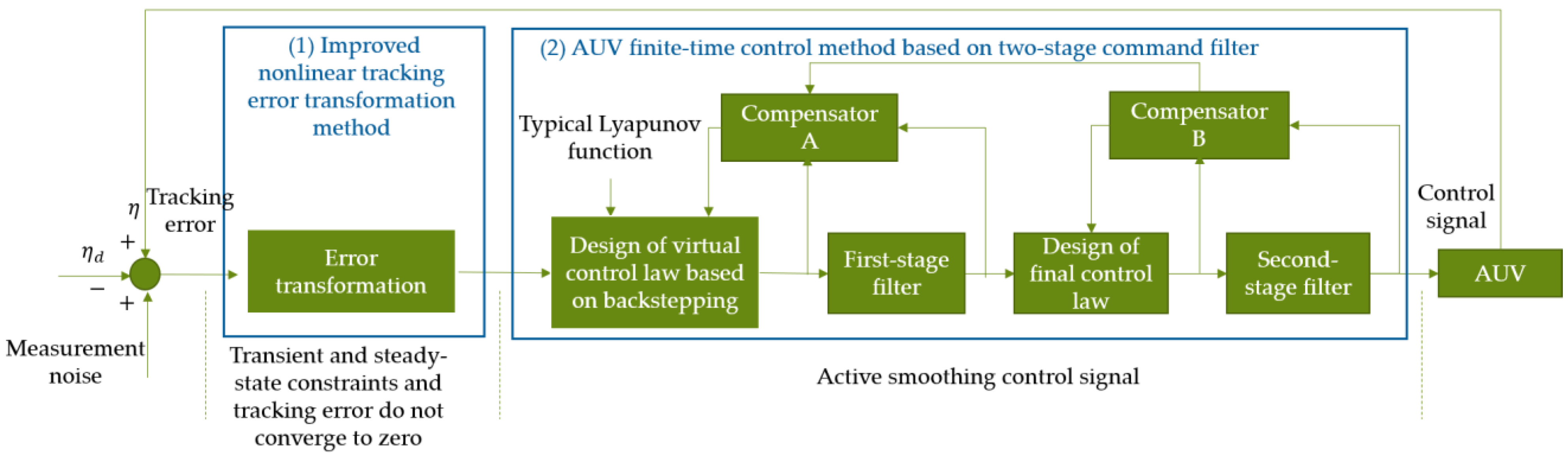
In order to ensure that the AUV tracking error meets the transient and steady-state performance constraints without converging to zero, an improved nonlinear tracking error transformation method is proposed in this paper. Different from previous studies [28,31], which used error transformation and the Lyapunov function in coordination to achieve this goal, we do not need to design a Lyapunov function but only to carry out nonlinear transformation of tracking errors based on allowable error variables, hyperbolic tangent functions, and performance functions. The objective can be realized by stabilizing the transformed error variable.

(2)

Aiming at the problem of strong fluctuation of the control signal when tracking an AUV region with measurement noise, a finite-time control method based on a two-stage command filter is proposed in this paper. Different from the traditional method, which directly uses the control law derived from the backstep method as the control signal, in this paper we adopt a finite-time sliding mode differentiator to filter the virtual and final control laws and design a finite-time compensator to compensate the filtering loss and stabilize the closed-loop system. Among them, the filtered final control law is used as the control signal to reduce the fluctuation of control signal caused by measurement noise.

The rest of the paper is organized as follows: Section 2 presents an analysis of the problems with the traditional method and gives the preliminaries. Section 3 introduces the ideas of this paper and explains the differences from the traditional methods, describes the concrete implementation process, and presents the completed stability proof of the closed-loop system. In Section 4, the method proposed in this paper is analyzed via simulation to verify its effectiveness. Section 5 gives the conclusion of this paper.

2. Problem Statement and Preliminaries

In this section, we first examine the issues and underlying factors present in traditional methods, and then provide the essential preliminary knowledge necessary to implement the methodologies presented in this paper.

2.1. Analysis of the Existing Problems and Their Causes in Traditional Methods

The control signal when using the traditional region tracking method [28,31] will produce strong fluctuations in the presence of measurement noise. An analysis of the cause of this problem shows that no matter what task the AUV performs, it needs to obtain its position information in real time [39]. A Doppler sensor is often used to obtain the velocity and position information of an AUV. Because its stability and measurement accuracy are easily affected by the marine environment, the status information obtained by an AUV contains measurement noise [40]. The control law derived from the traditional method [28,31] is directly assigned to the actuator (thruster) for execution as a control signal. When there is measurement noise, the state information obtained by the AUV will contain the noise information, and then the control law derived from the state information will contain the noise information. Moreover, the noise will be further amplified by the inertia matrix in the model during the derivation of the control law, so the phenomena of highly fluctuating frequency and large amplitude change will occur when the derived control law is directly taken as the control signal. The method based on error transformation in [31] reduces the sensitivity of the control signal to the actual tracking error, and thus reduces the influence of noise on the fluctuation of the control signal to a certain extent. However, this method cannot realize active regulation of the control signal, such as high-frequency removal and filtering of the control signal.

2.2. Preliminaries

(1)

Dynamic model

The controller design involves specific control objects. ODIN AUV is a typical AUV with an open dynamic model, and many studies have taken this AUV as the object [22,41]. In this paper, the AUV is used as the object to design the controller and for verification through a simulation experiment.

The dynamic model of ODIN AUV is

$$\begin{array}{l}\dot{\eta }=J(\eta )v\\ M\dot{v}+C_{RB}(v)v+C_A(v_r)v_r+D(v_r)v_r+G(\eta )=\tau \end{array}$$

(1)

where $\eta$ is a $6\times 1$ vector, which represents the position and attitude of the AUV with respect to the geodetic coordinate system; $v$ is a $6\times 1$ vector, which represents the linear velocity and angular velocity of the AUV with respect to the body coordinate system; $v_r=v-v_c$, and $v_c$ is a $6\times 1$ vector, representing the and angular velocity of the current relative to the coordinate system of the boat body; $J$ is a $6\times 6$ coordinate transformation matrix between the geodetic and boat coordinate systems; $M$ is a $6\times 6$ inertia matrix including the additional mass; $C_{RB}$ and $C_A$ are matrices which represent the rigid bod, hydrodynamic, and Coriolis force terms, respectively; $D$ is a $6\times 6$ hydrodynamic resistance matrix; $G$ is a $6\times 6$ restoring force matrix; and $\tau$ is the control force and moment acting on the center of gravity of the AUV. More details of these parameters are given in [42,43].

(2)

Lemma and assumption

Lemma 1

[44]. For any given normal numbers $m$, $n$, and $w$, the following inequality holds.

$$|x{|}^m|y{|}^n\le \frac{m}{m+n}w|x{|}^{m+n}+\frac{m}{m+n}{w}^{-\frac{m}{n}}|y{|}^{m+n}$$

where $x$ and $y$ are any real numbers.

Lemma 2

[45]. For any $x\in R$ and $\omega >0$, the following inequality holds.

$$0\le |x|-x\tan (\frac{x}{\omega })\le \varpi$$

where $\varpi =\delta \omega$ and $\delta =0.2785$.

Lemma 3

[46]. Consider the system $\dot{x}=f(x)$ . Suppose $V(x)$ is a smooth positive definite function of class C, if $V(x)$ satisfies $\dot{V}(x)\le -{\beta }_{1}V(x)-{\beta }_2{V}^P(x)+\chi$, where $V(0)=0$, ${\beta }_1,{\beta }_2>0$, $0<P<1$, and $0<\chi <\infty$; then the equilibrium point of system $\dot{x}=f(x)$ is finite-time $T=\max \{\frac{1}{\gamma {\beta }_1(1-P)}\ln \frac{\gamma {\beta }_1{V}^{1-P}(x_0)+{\beta }_2}{{\beta }_2},\frac{1}{{\beta }_1(1-P)}\ln \frac{{\beta }_1{V}^{1-P}(x_0)+\gamma {\beta }_2}{\gamma {\beta }_2}\}$ uniform and finally bounded, and the system state converges to the set $\Omega =\min \{\frac{\chi }{(1-\gamma ){\beta }_1},{(\frac{\chi }{(1-\gamma ){\beta }_2})}^{\frac{1}{P}}\}$ of the equilibrium domain, where $0<\gamma <1$.

Assumption 1

[47]. The interference force and torque on the AUV center of gravity are bounded:

$$\left|\right|d\left|\right|\le {\epsilon }_d$$

where  ${\epsilon }_d$  is a positive constant.

In this section, the shortcomings of traditional methods are analyzed, and the preliminaries required for implementing this method are given. The idea, implementation process and stability analysis of the AUV finite-time region tracking control method based on command filter proposed in this paper are described in detail.

3. AUV Finite-Time Region-Tracking Control Method Based on Command Filter

Based on the problems and their causes in traditional methods described in Section 2.1, in this section, we first introduce the idea of this method and describe the differences between it and traditional methods in detail. We decompose the proposed method into two sub-methods based on its concept: (1) An improved nonlinear tracking error transformation method and (2) an AUV finite-time control method based on two-stage command filter. Then we describe the implementation process in detail. Finally, the stability of the closed-loop system is analyzed based on the Lyapunov function method.

3.1. The Idea of This Method and Difference between This Method and Traditional Method

3.1.1. Idea of the Method in This Paper

The idea of the method is to ensure that the tracking error of the AUV satisfies the constraint of transient and steady-state performance without converging to zero and to solve the problem of strong fluctuation of the control signal in the traditional method described in Section 2.1. The intention is to decompose the above objectives into two sub-objectives: Make tracking errors meet the constraint requirements and smooth the control signals. Based on the two sub-objectives, two methods are proposed as solutions: (1) an improved nonlinear tracking error transformation method and (2) an AUV finite-time control method based on two-stage command filter. The overall idea of this paper is shown in Figure 1.

In Figure 1, the two blue wireframes represent the two sub-methods in the paper, and the text below the blue wireframes indicates the goals achieved by each sub-method. The ideas of each sub-method are described in detail as follows:

(1)

Improved nonlinear tracking error transformation method

Firstly, the relative position between tracking error and performance function is expressed in the form of inequality. Then, the concept of admissible error is introduced (that is, tracking error is considered to meet the requirements of regional tracking within the admissible error) to rewrite the constraint inequality. Finally, the hyperbolic tangent and quadratic functions are used to nonlinearly transform the inequality. A new error variable with an infinite interval domain and a continuous first derivative is obtained. In summary, based on the improved nonlinear tracking error transformation method, the constraint problem of tracking errors is transformed into a stability problem of the new error variable. The next step is to design the control law to stabilize the new error variable to ensure that the AUV tracking error meets the transient and steady-state performance constraints without converging to zero.

(2)

AUV finite-time control method based on two-stage command filter

In order to reduce the strong fluctuation of the control signal caused by measurement noise, we used a finite-time sliding mode differentiator to filter the virtual control law and the final control law in the backstep method and took the filtered final control law as the control signal so as to achieve the purpose of smoothing the control signal. In the above filtering process, considering the signal loss caused by filtering and the influence on system stability, a finite-time compensator was designed to compensate the filtering loss and ensure the stability of the closed-loop system. In addition, the control signal can be adjusted actively by adjusting the parameters of the finite-time sliding mode differentiator.

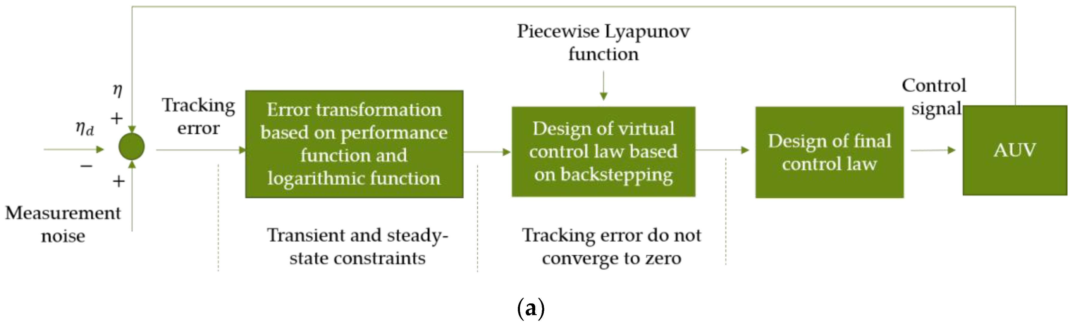
3.1.2. Difference between This Method and Traditional Method

To show the contribution of this paper more clearly, the design ideas of traditional methods are given in Figure 2, and the differences between the methods in this paper and those in the literature are described.

Figure 2 shows the design ideas of the region tracking method in previous studies [28,31]. Summarizing Figure 1 and Figure 2, the method in this paper differs from the traditional method in the following two aspects:

(1)

Treatment of error variables

The method of error transformation and the Lyapunov function were adopted in [28,31] to ensure that the AUV tracking error would meet performance constraints and not converge to zero. As can be seen from Figure 2a,b, the difference between the two studies is that in [28], the authors chose to ensure that performance constraints are met in the error transformation stage, and then the tracking error does not converge to zero based on a piecewise Lyapunov function, while in [31], the authors chose to ensure that the error does not converge to zero in the error transformation stage. Then, the performance constraint is realized based on the Lyapunov function.

Different from [28,31], the method in this paper can ensure that the AUV tracking error meets the performance constraints and does not converge to zero in the error transformation stage, which avoids the steps involved in the traditional method requiring a special design for the Lyapunov function, simplifies the derivation process of the control law, and increases the flexibility of the controller design.

(2)

Smoothing of control signals

The authors of [28] did not design the control signal fluctuation caused by measurement noise. The authors of [31] made the transformed error variable smaller than the real tracking error through nonlinear transformation of the tracking error, as shown in Figure 2b. This operation not only ensures that the tracking error mentioned in (1) does not have to converge to zero but also reduces the sensitivity of the control signal to the tracking error. Considering that measurement noise is superimposed on the tracking error, the purpose of reducing the influence of noise on the control signal fluctuation is realized indirectly.

Differently from the purpose of smoothing control signals by reducing the sensitivity of control signals to tracking errors in [31], in terms of active smoothing control signals, in this paper we added a two-stage command filter after the designed virtual and final control laws and used the filter to smooth control signals with the optimal asymptotic feature of input noise. In addition, because of the adjustability of filter parameters, the proposed method also can actively adjust signal fluctuations.

3.2. Implementation Process of Proposed Method

To realize the method presented in this paper, the tracking errors are first converted based on the improved nonlinear tracking error transformation method, and then the AUV finite-time control method with two-stage command filter is used to derive the control law to stabilize the new error variables.

3.2.1. Improved Nonlinear Tracking Error Transformation Method

The method presented in this section is to transform the bounded problem of tracking error into a stability problem so that the traditional controller design method can be used directly. First, the performance requirements of tracking errors are written in the form of constraint inequalities, and then the inequalities are modified by introducing admissible error variables to meet the requirements of regional tracking. Finally, the inequalities are nonlinear transformed to obtain new error variables.

(1)

Construct the performance constraint inequality

In this paper, a prescribed performance function is used to constrain the transient and steady-state performance of an AUV; that is, the designed controller should satisfy the constraint inequality of Equation (2):

$$\begin{array}{ccc}-{\delta }_i{\rho }_i(t)<e_i(t)<-{\rho }_i(t)& if& e_i(0)\ge 0\\ -{\rho }_i(t)<e_i(t)<-{\delta }_i{\rho }_i(t)& if& e_i(0)<0\end{array}$$

(2)

where subscript $i\in [1,2,3,4,5,6]$ represents the $i$th component of each vector, and the same below; $e(t)=\eta -{\eta }_d$ represents the tracking error of the AUV, ${\eta }_d$ represents the expected trajectory and attitude vector; $\delta \in [0,1]$ is the overshoot limit parameter; and $\rho (t)$ is the prescribed performance function of finite-time convergence, which can be expressed as

$$\rho (t)=\left\{\begin{array}{ccc}{({\rho }_0^{\tau }-\tau \lambda t)}^{1/\tau }+{\rho }_T& if& 0\le t<T\\ {\rho }_T& if& t\ge T\end{array}\right.$$

(3)

where $\rho (0)$ and ${\rho }_T$ represent the values of $\rho (t)$ at the initial time and time $T$; ${\rho }_0^{}$, $\tau$ and $\lambda$ need to be selected according to the values of ${\rho }_T$, $T$ and $\rho (0)$; there are ${\rho }_0=\rho (0)-{\rho }_T$, $\tau \lambda ={\rho }_0^{\tau }/T$ and, $\tau =q_1/q_2\in (0,1)$, where $q_1$ and $q_2$ are positive odd and positive even, respectively. Note that the value of $\rho (0)$ should be greater than the absolute value of the initial tracking error of the AUV.

To ensure that tracking errors meet the requirements in Equation (2), the following transformations are performed:

$$\begin{array}{ccc}-1<\frac{2e_i(t)}{(1+{\delta }_i){\rho }_i(t)}+\frac{{\delta }_i-1}{1+{\delta }_i}<1& if& e_i(0)\ge 0\\ -1<\frac{2e_i(t)}{(1+{\delta }_i){\rho }_i(t)}+\frac{1-{\delta }_i}{1+{\delta }_i}<1& if& e_i(0)<0\end{array}$$

(4)

Then, we define the variable ${\vartheta }_i$ and rewrite Equation (4) as

$${\vartheta }_i=\left\{\begin{array}{ccc}\frac{2e_i(t)}{(1+{\delta }_i){\rho }_i(t)}+\frac{{\delta }_i-1}{1+{\delta }_i}& if& e_i(0)\ge 0\\ \frac{2e_i(t)}{(1+{\delta }_i){\rho }_i(t)}+\frac{1-{\delta }_i}{1+{\delta }_i}& if& e_i(0)<0\end{array}\right.$$

(5)

where, ${\delta }_i\in [0,1]$ is the overshoot limit parameter; when ${\delta }_i=0$, the closed-loop system is not allowed to generate overshoot. As can be seen from Equation (5), if variable ${\vartheta }_i$ satisfies $-1<{\vartheta }_i<1$, the tracking error is within the designed performance constraint range.

The equivalence proof in this sub-section has been completed in the literature, see Ref. [36] for details.

(2)

Introduce tolerance error to rewrite performance constraint inequality

Considering the regional tracking method to reduce precision in exchange for energy consumption and controller burden as the starting point, we introduce the concept of allowable error; that is, we set an allowable range of tracking error, and if the tracking error is within this range, it is considered to meet the tracking requirements. We set the allowable error range based on the range of variable ${\vartheta }_i$:

$$-1<{\vartheta }_i<{\vartheta }_{t\min i}<0<{\vartheta }_{t\max i}<{\vartheta }_i<1$$

(6)

If the allowable errors on both sides of the equilibrium point satisfy ${\vartheta }_{t\min i}=-{\vartheta }_{t\max i}$, Equation (6) can be written as

$$\left|{\vartheta }_{ti}\right|<\left|{\vartheta }_i\right|<1$$

(7)

The previous section has obtained the result that the tracking error does not exceed the performance constraint range. If Equation (7) is satisfied, the goal of tracking error convergence to zero can be further achieved, which is the design goal of region tracking. The equivalence proof is shown in Theorem 1.

Theorem 1.

Considering the variable definition (Equation (5)), if there is an inequality constraint (Equation (7)), then the tracking error $e_i$ is constrained to a region outside the zero point, with the boundary being:

$$\begin{array}{ccc}{e}_i(t)\ge \frac{1}{2}{\rho }_i(t)(1+{\delta }_i){\vartheta }_{t\max i}+\frac{1}{2}{\rho }_i(t)(1-{\delta }_i)>0& if& e_i(0)\ge 0\\ e_i(t)\le -\frac{1}{2}{\rho }_i(t)(1+{\delta }_i){\vartheta }_{t\min i}-\frac{1}{2}{\rho }_i(t)(1-{\delta }_i)<0& if& e_i(0)<0\end{array}$$

Proof 1.

According to the restrictions ${\vartheta }_{t\max i}$ and ${\vartheta }_{t\min i}$ on the variable ${\vartheta }_i$ in Equation (6), Equation (5) is rewritten as

$$\begin{array}{ccc}{\vartheta }_{t\max i}\le \frac{2e_i(t)}{(1+{\delta }_i){\rho }_i(t)}+\frac{{\delta }_i-1}{1+{\delta }_i}& if& e_i(0)\ge 0\\ {\vartheta }_{t\min i}\le -\frac{2e_i(t)}{(1+{\delta }_i){\rho }_i(t)}+\frac{{\delta }_i-1}{1+{\delta }_i}& if& e_i(0)<0\end{array}$$

Rewritten as

$$\begin{array}{ccc}{e}_i(t)\ge \frac{1}{2}{\rho }_i(t)(1+{\delta }_i){\vartheta }_{t\max i}+\frac{1}{2}{\rho }_i(t)(1-{\delta }_i)& if& e_i(0)\ge 0\\ e_i(t)\le -\frac{1}{2}{\rho }_i(t)(1+{\delta }_i){\vartheta }_{t\min i}-\frac{1}{2}{\rho }_i(t)(1-{\delta }_i)& if& e_i(0)<0\end{array}$$

According to the definition of $\rho (t)$ and the definition of the overshoot limit parameter ${\delta }_i$, it can be seen that

$$\begin{array}{cc}\frac{1}{2}{\rho }_i(t)(1+{\delta }_i){\vartheta }_{t\max i}+\frac{1}{2}{\rho }_i(t)(1-{\delta }_i)>0& \\ \frac{1}{2}{\rho }_i(t)(1+{\delta }_i){\vartheta }_{t\min i}+\frac{1}{2}{\rho }_i(t)(1-{\delta }_i)>0& \end{array}$$

Therefore, if Equation (7) holds, the tracking error $e(t)$ is constrained to be near the origin, with a boundary of:

$$\begin{array}{ccc}{e}_i(t)\ge \frac{1}{2}{\rho }_i(t)(1+{\delta }_i){\vartheta }_{t\max i}+\frac{1}{2}{\rho }_i(t)(1-{\delta }_i)>0& if& e_i(0)\ge 0\\ e_i(t)\le -\frac{1}{2}{\rho }_i(t)(1+{\delta }_i){\vartheta }_{t\min i}-\frac{1}{2}{\rho }_i(t)(1-{\delta }_i)<0& if& e_i(0)<0\end{array}$$

(3)

Nonlinear transformation of constrained inequalities

The design goal of the control law is usually to converge a bounded error variable with a continuous first derivative. In order to make the control target satisfy the constraint conditions (Equation (8)), a mapping of the variable ${\vartheta }_i$ is required, and the new error variable after mapping should satisfy the requirements of boundedness and continuous first derivative.

Theorem 2.

Considering the variable definition (Equation (5)) and the constraint condition (Equation (7)), perform the nonlinear transformation on ${\vartheta }_i$ in (Equation (8)). Then ${\sigma }_{ri}$ is bounded and the first derivative is continuous, and ${\sigma }_{ri}$ is bounded equivalent to the constraint condition (Equation (8)) being satisfied.

$${\sigma }_{ri}=\left\{\begin{array}{ccc}{\epsilon }_{i}sign({\sigma }_i){(|{\sigma }_i|-sign({\sigma }_i){\sigma }_{\max i})}^2& if& \left|{\sigma }_i\right|>{\sigma }_{\max i}\\ 0& if& \left|{\sigma }_i\right|\le {\sigma }_{\max i}\end{array}\right.$$

(8)

where  ${\sigma }_i=\arctan h({\vartheta }_i)$,  ${\sigma }_{\max i}=\arctan h({\vartheta }_{t\max i})$, and  ${\epsilon }_i>0$  are design parameters used to adjust the mapping relationship between the tracking error and the new error variable.

Proof 2.

From Equations (1) and (2) in Section 3.2.1, it can be seen that the variable ${\vartheta }_i$ monotonically increases with respect to tracking error $e_i$, and its boundary is constrained by Equation (7). Considering the properties of the inverse hyperbolic tangent function $\underset{{\sigma }_i\to +\infty }{\lim }\tan h({\sigma }_i)=1$ and $\underset{{\sigma }_i\to -\infty }{\lim }\tan h({\sigma }_i)=-1$. Based on the function ${\sigma }_i=\arctan h({\vartheta }_i)$, the variable ${\vartheta }_i$ is transformed into a new interval. At this point, it can be seen that as long as the bound of ${\sigma }_i$ is satisfied, the constraint (Equation (7)) holds.

Based on the above transformation, it can be seen that the variable ${\sigma }_i$ has a jump discontinuity at the point zero ($\underset{{\sigma }_i\to 0^{+}}{\lim }{\sigma }_i={\sigma }_{\max i}$, $\underset{{\sigma }_i\to 0^{-}}{\lim }{\sigma }_i=-{\sigma }_{\max i}$, and $-{\sigma }_{\max i}\ne {\sigma }_{\max i}$) and cannot be directly used for the design of control laws. After the nonlinear transformation (Equation (8)) proposed in this paper, there is $\underset{{\sigma }_i\to {\sigma }_{\max i}}{\lim }{\sigma }_{ri}=\underset{{\sigma }_i\to -{\sigma }_{\max i}}{\lim }{\sigma }_{ri}=0$, and the part of Equation (8) in $\left|{\sigma }_i\right|>{\sigma }_{\max i}$ is a typical quadratic function. Therefore, after transformation, the variable ${\sigma }_{ri}$ has the characteristic of continuous first derivative, which can be used for the design of control laws. Further considering that the transformation does not change the monotonicity and boundedness of the variable ${\sigma }_i$, as long as ${\sigma }_i$ is bounded, the constraint condition (Equation (7)) holds. That is, the constraint problem in Equation (7) is equivalently transformed into a bounded problem of variable ${\sigma }_{ri}$.

In order to achieve control of the AUV under performance constraints, it is necessary to design a control law that stabilizes and converges the variable ${\sigma }_{ri}$. The following section describes the design of the control law in this paper.

3.2.2. AUV Finite-Time Control Method Based on Second-Stage Command Filter

In the above section, the proposed nonlinear error transformation method proposed is adopted to transform the bounded constraint problem of tracking error into the stability problem of variables. In this section, the control law is derived to stabilize variables based on the proposed AUV finite-time control method with the two-stage command filter. The method is implemented in two steps: Step 1: Design virtual control law and compensator $A$; Step 2: Design final control law and compensator $B$. These are described in detail below.

Step 1: Design the virtual control law and compensator $A$.

Due to the introduction of command filters in the derivation process of the control law, a deviation between the filter output and the input is caused. Therefore, this paper defines compensator $A$ for the error variable ${\sigma }_r$ and compensator $B$ for the virtual error variable ${\sigma }_2$. The specific expressions for compensators $A$ and $B$ will be given below. In order to stabilize the error ${\sigma }_r$ and compensator $A$ and stabilize the error ${\sigma }_2$ and compensator $B$, the following virtual composite variables are designed:

$$\begin{array}{l}{z}_1={\sigma }_r-A\\ z_2={\sigma }_2-B\end{array}$$

(9)

where ${\sigma }_r={[{\sigma }_{r1},{\sigma }_{r2},{\sigma }_{r3},{\sigma }_{r4},{\sigma }_{r5},{\sigma }_{r6}]}^T$ and ${\sigma }_2=v-v_{ac}$ are the virtual errors and $v_{ac}$ will be defined later; $A$ and $B$ are compensators $A$ and $B$, designed in this paper; and $v_{ac}$, $A$, $B$, $z_1$ and $z_2$ are all $6\times 1$ vectors.

To stabilize variable $z_1$, a typical Lyapunov function is selected:

$$V_1=0.5z_1^T{z}_1$$

(10)

Consider Equations (1) and (8) and take the derivative of Equation (10):

$$\begin{array}{l}{\dot{V}}_1=z_1^T({\dot{\sigma }}_r-\dot{A})\\ =z_1^T(r_1+r_2(Jv-{\dot{\eta }}_d)-\dot{A})\end{array}$$

(11)

where $r_1={[r_{11},r_{12},r_{13},r_{14},r_{15},r_{16}]}^T$, $r_2={[r_{21},r_{22},r_{23},r_{24},r_{25},r_{26}]}^T$, $r_{1i}=-2{\epsilon }_i(\arctan h(\frac{e_i}{{\rho }_i(t)})-sign({\sigma }_i){\sigma }_{\max i})\frac{e_i{\dot{\rho }}_i(t)}{{\rho }_i{(t)}^2-e_i^2}$, $r_{2i}=2{\epsilon }_i(\arctan h(\frac{e_i}{{\rho }_i(t)})-sign({\sigma }_i){\sigma }_{\max i})\frac{{\rho }_i(t)}{{\rho }_i{(t)}^2-e_i^2}$, $i\in [1,\dots ,6]$.

In order to improve the smoothness of the system output and avoid the problem of parameter explosion caused by the derivative of the virtual control law below, we designed a first-stage filtering link. Since the two-stage sliding mode differentiator has the property of asymptotic convergence to noise, we adopted the differentiator pair for filtering, and its structure is as follows:

$$\begin{array}{l}{\dot{v}}_{ac}=-r_3|v_{ac}-v_c{|}^{0.5}sign(v_{ac}-v_c)+v_2\\ {\dot{v}}_2=-r_{4}sign(v_2-{\dot{v}}_{ac})\end{array}$$

(12)

where $r_3,r_4>0$ indicates the design parameters, $v_c$ is the virtual control law, $v_{ac}$ is the filtered control signal, and the filtering error is represented by $q_{ac}=v_{ac}-v_c$.

Considering the above filtering errors and virtual errors, Equation (11) can be written as

$${\dot{V}}_1=z_1^T(r_1+r_2(J({\sigma }_2+q_{ac}+v_c)-{\dot{\eta }}_d)-\dot{A})$$

(13)

The virtual control law $v_c$ and finite-time compensator $B$ designed in this paper are as follows:

$$v_c=-\frac{k_1{J}^{-1}}{r_2}{\sigma }_r-\frac{k_v{J}^{-1}}{r_2}{\zeta }^P(z_1)-J^{-1}(\frac{r_1}{r_2}-{\dot{\eta }}_d)$$

(14)

$$\dot{A}=-k_{1}A-a_1{\zeta }^P(A)+r_{2}JB+r_{2}J{q}_{ac}$$

(15)

where $k_1,k_v>0$ indicates the design parameters, $\zeta {(·)}^P={(·)}^P{\tanh }^{P+1}(\frac{·}{\omega })$, $0<P<1$ and $\omega$ is a normal number with a small value.

Substitute Equations (14) and (15) into Equation (13), then:

$$\begin{array}{l}{\dot{V}}_1=z_1^T(r_1+r_{2}J{\sigma }_2+r_{2}J{q}_{ac}+r_{2}J(-\frac{k_1{J}^{-1}}{r_2}{\sigma }_r-\frac{k_v{J}^{-1}}{r_2}{\zeta }^P(z_1)-J^{-1}(\frac{r_1}{r_2}-{\dot{\eta }}_d))\\ -r_2{\dot{\eta }}_d+k_{1}A+a_1{\zeta }^P(A)-r_{2}JB-r_{2}J{q}_{ac})\\ =z_1^T(r_{2}J{\sigma }_2-k_1{\sigma }_r-k_v{\zeta }^P(z_1)+k_{1}A+a_1{\zeta }^P(A)-r_{2}JB)\end{array}$$

(16)

Based on Equations (9) and (16) can be rewritten as:

$${\dot{V}}_1=-k_1{z}_1^T{z}_1-k_v{z}_1^T{\zeta }^P(z_1)+z_1^T{r}_{2}J{z}_2+a_1{z}_1^T{\zeta }^P(A)$$

(17)

Step 2. Design the final control law and compensator $B$.

To design the final control law and compensator $B$ to stabilize the whole controller, select the Lyapunov function:

$$V_2=0.5z_2^T{z}_2$$

(18)

Take the derivative of Equation (18) and consider model (Equation (1)) and filtering error as follows:

$${\dot{V}}_2=z_2^T(M^{-1}{\tau }_c-M^{-1}F+M^{-1}d-{\dot{v}}_{ac}-\dot{B})$$

(19)

where $F=C_{RB}(v)v+C_A(v)v+D(v)v+G(\eta )$ and $d$ is a $6\times 1$ vector, representing the interference force and torque acting on the AUV’s center of gravity, mainly including ocean current, propeller failure and other influences. To be consistent with the corresponding meanings of symbols in step 1, $\tau$ in the dynamic model is written as ${\tau }_c$ here, indicating that the control law is the design control law.

In order to actively smooth the control signal, a second-stage filtering link is added after the final control law ${\tau }_c$. The structure of the command filter selected by this link is the same as that in Step 1, as follows:

$$\begin{array}{l}{\dot{\tau }}_{ac}=-r_5|{\tau }_{ac}-{\tau }_c{|}^{0.5}sign({\tau }_{ac}-{\tau }_c)+{\tau }_2\\ {\dot{\tau }}_2=-r_{6}sign({\tau }_2-{\dot{\tau }}_{ac})\end{array}$$

(20)

where $r_5,r_6>0$ indicates the design parameters, ${\tau }_{ac}$ is the filtered control signal, and the filtering error is represented by $q_{\tau ac}={\tau }_{ac}-{\tau }_c$.

The final control law ${\tau }_c$ and finite-time compensator $B$ designed in this paper are as follows:

$${\tau }_c=-M{z}_1{r}_{2}J-k_{\tau }M{\zeta }^P(z_2)+F-\widehat{d}+M{\dot{v}}_{ac}-M{k}_2{\sigma }_2+q_{\tau ac}$$

(21)

$$\dot{B}=-k_{2}B-b_1{\zeta }^P(B)+M^{-1}{q}_{\tau ac}$$

(22)

where $k_2,k_{\tau }>0$ is the design parameter and which $\widehat{d}$ is obtained by using the finite-time disturbance observer in [48]. To prepare for the stability proof in the next part, Equations (21) and (22) are substituted into Equation (19), and we can obtain:

$$\begin{array}{l}{\dot{V}}_2=z_2^T(-z_1{r}_{2}J-k_{\tau }{\zeta }^P(z_2)+M^{-1}F-M^{-1}\widehat{d}+{\dot{v}}_{ac}-k_2{\sigma }_2+M^{-1}{q}_{\tau ac}\\ -M^{-1}F+M^{-1}d-{\dot{v}}_{ac}+k_{2}B+b_1{\zeta }^P(B)-M^{-1}{q}_{\tau ac})\\ =-z_2^T{z}_1{r}_{2}J-k_2{z}_2^T{z}_2-k_{\tau }{\zeta }^P(z_2)-z_2^T{M}^{-1}(\widehat{d}-d)+b_1{z}_2^T{\zeta }^P(B)\end{array}$$

(23)

Based on the above error transformation and controller design processes, the proposed method was implemented, and the control law (Equations (14) and (21)) and compensator (Equations (15) and (22)) required by the proposed method were obtained. In the next section, the stability of the closed-loop system is analyzed based on the control law and compensator obtained by the proposed method.

3.3. Stability Analysis of Closed Loop System

This section analyzes the closed-loop system based on Lyapunov stability theory, and the main result is expressed by Theorem 3.

Theorem 3.

Considering the AUV system (Equation (1)) and Assumption 1, under the action of the control law (Equations (14), (15), (21) and (22)), the error variable  ${\sigma }_{ri}$ can achieve region tracking with transient and steady-state performance constraints in a finite time, and its convergence region is $\Omega =\min \{\frac{\chi }{(1-\gamma ){\beta }_1},{(\frac{\chi }{(1-\gamma ){\beta }_2})}^{\frac{1}{P}}\}$, $0<\gamma <1$.

Proof 3.

To prove the stability of the closed-loop system (including the stability of the compensator), the Lyapunov function is selected:

$$V=V_1+V_2+0.5A^2+0.5B^2$$

(24)

Then we take the derivative of Equation (24), and substitute Equations (15), (17), (22) and (23):

$$\begin{array}{l}{\dot{V}}_3=-k_1{z}_1^T{z}_1-k_v{(z_1^T\tanh (\frac{z_1}{\omega }))}^{P+1}-k_2{z}_2^T{z}_2-k_{\tau }{(z_2^T\tanh (\frac{z_2}{\omega }))}^{P+1}\\ +a_1{z}_1^T{\zeta }^P(A)+b_1{z}_2^T{\zeta }^P(B)-z_2^T{M}^{-1}(\widehat{d}-d)\\ +A(-k_{1}A-a_1{\zeta }^P(A)+r_{2}JB+r_{2}J{q}_{ac})+B(-k_{2}B-b_1{\zeta }^P(B)+M^{-1}{q}_{\tau ac})\end{array}$$

(25)

According to Young’s inequality and Lemma 1, the following inequality is established:

$$\begin{array}{l}{a}_1{z}_1^T{\zeta }^P(A)\le 0.5z_1^T{z}_1+0.5a_1^2((1-p)p^{\frac{p}{1-p}}+A^2)\\ b_1{z}_2^T{\zeta }^P(B)\le 0.5z_2^T{z}_2+0.5b_1^2((1-p)p^{\frac{p}{1-p}}+B^2)\end{array}$$

(26)

Substitute Equation (26) into Equation (25):

$$\begin{array}{l}{\dot{V}}_3\le -k_1{z}_1^T{z}_1-k_v{(z_1^T\tanh (\frac{z_1}{\omega }))}^{P+1}-k_2{z}_2^T{z}_2-k_u{(z_2^T\tanh (\frac{z_2}{\omega }))}^{P+1}-z_2^T{M}^{-1}(\widehat{d}-d)\\ +0.5z_2^T{z}_2+0.5b_1^2((1-p)p^{\frac{p}{1-p}}+B^2)+0.5z_1^T{z}_1+0.5a_1^2((1-p)p^{\frac{p}{1-p}}+A^2)\\ -k_1{A}^2-a_1{(A_1^T\tanh (\frac{A_1}{\omega }))}^{P+1}+A{r}_{2}JB+A{r}_{2}J{q}_{ac}-k_2{B}^2-b_1{(B_1^T\tanh (\frac{B_1}{\omega }))}^{P+1}+B{M}^{-1}{q}_{\tau ac}\end{array}$$

(27)

According to the filter properties of the filter, it is assumed that $||q_{ac}||\le {\epsilon }_{q1}$ and $||q_{\tau ac,i}||\le {\epsilon }_{q2}$ exist, and combined with Assumption 1, partial function terms in Equation (25) are treated as follows:

$$\begin{array}{l}A{r}_{2}JB\le \frac{{\delta }^2}{2}||r_{2}J|{|}^2||A|{|}^2+\frac{1}{2{\delta }^2}||B|{|}^2\\ A{r}_{2}J{q}_{ac}\le \frac{{\delta }^2}{2}||r_{2}J|{|}^2||A|{|}^2+\frac{1}{2{\delta }^2}||{\epsilon }_{q1}|{|}^2\\ B{M}^{-1}{q}_{\tau ac}\le \frac{{\delta }^2}{2}||M^{-1}|{|}^2||B|{|}^2+\frac{1}{2{\delta }^2}||{\epsilon }_{q2}|{|}^2\\ -z_2^T{M}^{-1}(\widehat{d}-d)\le 0.5z_2^T{z}_2+0.5||M^{-1}|{|}^2||{\epsilon }_d|{|}^2\end{array}$$

(28)

In addition, according to Lemma 2, we continue to process the function term in Equation (27):

$$\begin{array}{l}-{(z_1^T\tanh (\frac{z_1}{\omega }))}^{P+1}\le \varpi +(2^P-1)z_1^2-|z_1{|}^{P+1}\\ -{(z_2^T\tanh (\frac{z_2}{\omega }))}^{P+1}\le \varpi +(2^P-1)z_2^2-|z_2{|}^{P+1}\\ -{(A^T\tanh (\frac{A}{\omega }))}^{P+1}\le \varpi +(2^P-1)A^2-|A{|}^{P+1}\\ -{(B^T\tanh (\frac{B}{\omega }))}^{P+1}\le \varpi +(2^P-1)B^2-|B{|}^{P+1}\end{array}$$

(29)

By substituting Equations (28) and (29) into (27), we obtain

$$\begin{array}{l}{\dot{V}}_3\le -(k_1-k_v(2^P-1)-0.5)z_1^T{z}_1-k_v|z_1{|}^{P+1}\\ -(k_2-k_{\tau }(2^P-1)-1)z_2^T{z}_2-k_{\tau }|z_2{|}^{P+1}\\ -(-0.5a_1^2+k_1-a_1(2^P-1)-{\delta }^2||r_{2}J|{|}^2)A^2-a_1|A{|}^{P+1}\\ -(-0.5b_1^2+k_2-b_1(2^P-1)-\frac{{\delta }^2}{2}||M^{-1}|{|}^2-\frac{1}{2{\delta }^2})B^2-b_1|B{|}^{P+1}\\ +\chi \\ \chi =k_v\varpi +k_{\tau }\varpi +0.5a_1^2(1-p)p^{\frac{p}{1-p}}+0.5b_1^2(1-p)p^{\frac{p}{1-p}}\\ +a_1\varpi +\frac{1}{2{\delta }^2}||{\epsilon }_{q1}|{|}^2+b_1\varpi +\frac{1}{2{\delta }^2}||{\epsilon }_{q2}|{|}^2+0.5||M^{-1}||{|}^2|{\epsilon }_d|{|}^2\end{array}$$

(30)

This can be further written in the following standard form:

$$\begin{array}{l}{\dot{V}}_3\le -{\beta }_1{V}_3-{\beta }_2{V}_3^{P_1}+\chi \\ {\beta }_1=\min \{2k_1-2k_v(2^P-1)-1,2k_2-2k_{\tau }(2^P-1)-1,-a_1^2+2k_1\\ -2a_1(2^P-1)-2{\delta }^2||r_{2}J|{|}^2,-b_1^2+2k_2-2b_1(2^P-1)-{\delta }^2||M^{-1}|{|}^2-\frac{1}{{\delta }^2}\}\\ {\beta }_2=\min \{2^{P_1}{k}_v,2^{P_1}{k}_{\tau },2^{P_1}{a}_1,2^{P_1}{b}_1\}\end{array}$$

(31)

where $P_1=\frac{P+1}{2}$.

According to lemma 3, the closed-loop system will converge to region $\Omega =\min \{\frac{\chi }{(1-\gamma ){\beta }_1},{(\frac{\chi }{(1-\gamma ){\beta }_2})}^{\frac{1}{P}}\}$, $0<\gamma <1$. in finite-time, which also means that the error variables ${\sigma }_r$ and ${\sigma }_2$ will stabilize to the equilibrium neighborhood in finite time. According to the improved nonlinear tracking error transformation method proposed in this paper, the transient and steady-state performance of the actual tracking error of AUV at this time meets the set performance function constraints, and the tracking error does not have to converge to zero.

This section describes the idea of the proposed method and how it differs from the traditional method and presents the concrete implementation process of the method and the proof of stability of the closed-loop system. The next section describes the comparative simulation experiments conducted to verify the AUV region tracking effect and the smoothness of control signals under the proposed method.

4. Simulation Experiment

This section verifies the effectiveness of command filter-based region tracking control for AUV with measurement noise by comparing simulation experiments of ODIN AUV. First, the authors present the simulation setting of the experiment in this paper. Then, they present the experimental results and an analysis of the comparison between this method and those in previous studies [28,31].

4.1. Simulation Settings

In this paper, consistently with the comparison literature [28,31], the ODIN AUV was used for the simulation experiment, and the same simulation settings were used: (1) thrust distribution matrix, (2) thruster dead zone and saturation, (3) ocean current, (4) noise, (5) fault, (6) expected trajectory, and (7) initial state of AUV.

The configurations and parameters were as follows:

(1)

Thrust distribution [28,31]: ODIN is an overdriven AUV composed of four horizontal thrusters and four verticals. In order to compare the input control signals of each thruster and subsequently conduct an energy consumption analysis, $\tau$ is written as $\tau =Eu$ in the dynamics model, where $E$ is a $6\times 8$ thrust distribution matrix, and $u$ is a $8\times 1$ vector, representing the thrust of eight thrusters. The expression is as follows:

$$E=\left[\begin{array}{cccccccc}s& -s& -s& s& 0& 0& 0& 0\\ s& s& -s& -s& 0& 0& 0& 0\\ 0& 0& 0& 0& -1& -1& -1& -1\\ 0& 0& 0& 0& Rs& Rs& -Rs& -Rs\\ 0& 0& 0& 0& Rs& -Rs& -Rs& Rs\\ R_z& -R_z& R_z& -R_z& 0& 0& 0& 0\end{array}\right]$$

where $s=\sin (\pi /4)$, $R=0.381$ and $R_z=0.508$.

(2)

Dead zone and saturation [31]: Dead zone and saturation are the actual constraints of thrust existence and were set as:

$$u_{si}=\left\{\begin{array}{c}150\\ u_i-10\\ 0\\ u_i+15\\ -100\end{array}\right.\begin{array}{cc}& \\ & \end{array}\begin{array}{c}{u}_i\ge 160\\ 160>u_i\ge 10\\ 10>u_i\ge -15\\ -15>u_i\ge -115\\ -115\ge u_i\end{array}$$

where $u_{si}$ is the propeller output considering dead zone and saturation factors.

(3)

Ocean current [31]: In order to get close to the real marine environment, the first-order Gauss–Markov process with Gaussian white noise (mean 1, variance 2) was used to simulate the amplitude of ocean current, and the integral of Gaussian white noise (mean 0, variance 50) was used to represent the phase angle of ocean current.

(4)

Noise [31]: In practical applications, a low-pass filter is used to reduce the overamplification effect caused by measurement noise. In this experiment, Gaussian noise (mean 0, variance 0.05) after a low-pass filter (2 rad/s) was added to the original position signal as the noisy position signal, and Gaussian noise (mean 0, variance 0.01) after a low-pass filter (1 rad/s) was added to the original velocity signal as the noisy speed signal.

(5)

Fault [31]: Considering the loss of thrust due to possible faults caused by long-term use of the thruster, it is assumed that failure of thruster T2 occurs; that is, the actual output of thruster T2 is only $(1-k_f)u_{s2}$, where

$$k_f=\left\{\begin{array}{c}0\\ 0.29/30(t-30)+0.01\sin (\pi /5(t-20))\\ 0.29+0.01\sin (\pi /(t-50))\end{array}\right.\begin{array}{cc}& \end{array}\begin{array}{c}0\le t<20\\ 20\le t<50\\ t\ge 50\end{array}.$$

(6)

Expected trajectory [31] is described as

$${\eta }_d={[3(1-\cos (0.15t)),3\sin (0.15t),-0.2t,0,0,0]}^T.$$

(7)

The initial state [31] of the AUV is: $\begin{array}{l}\eta (0)={[1,1,-1,\pi /18,\pi /18,\pi /9]}^T\\ \dot{\eta }(0)={[0.04,0.04,0.04,0.02,0.02,0.02]}^T\end{array}$.

Based on the above simulation preparation, experiments were carried out as described in the next section.

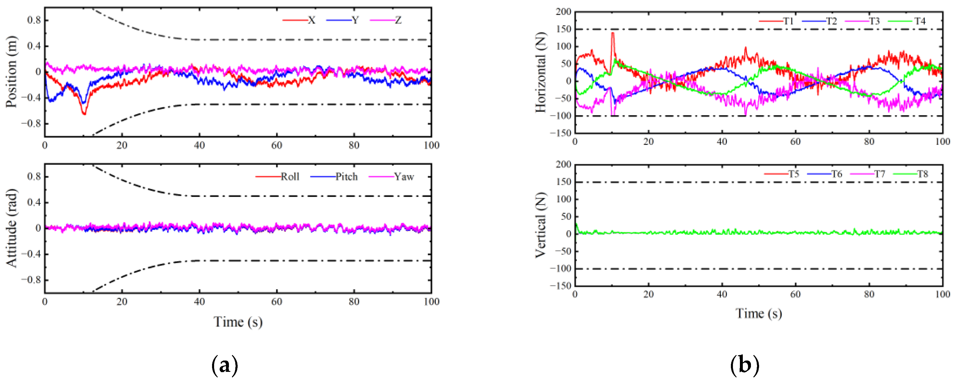
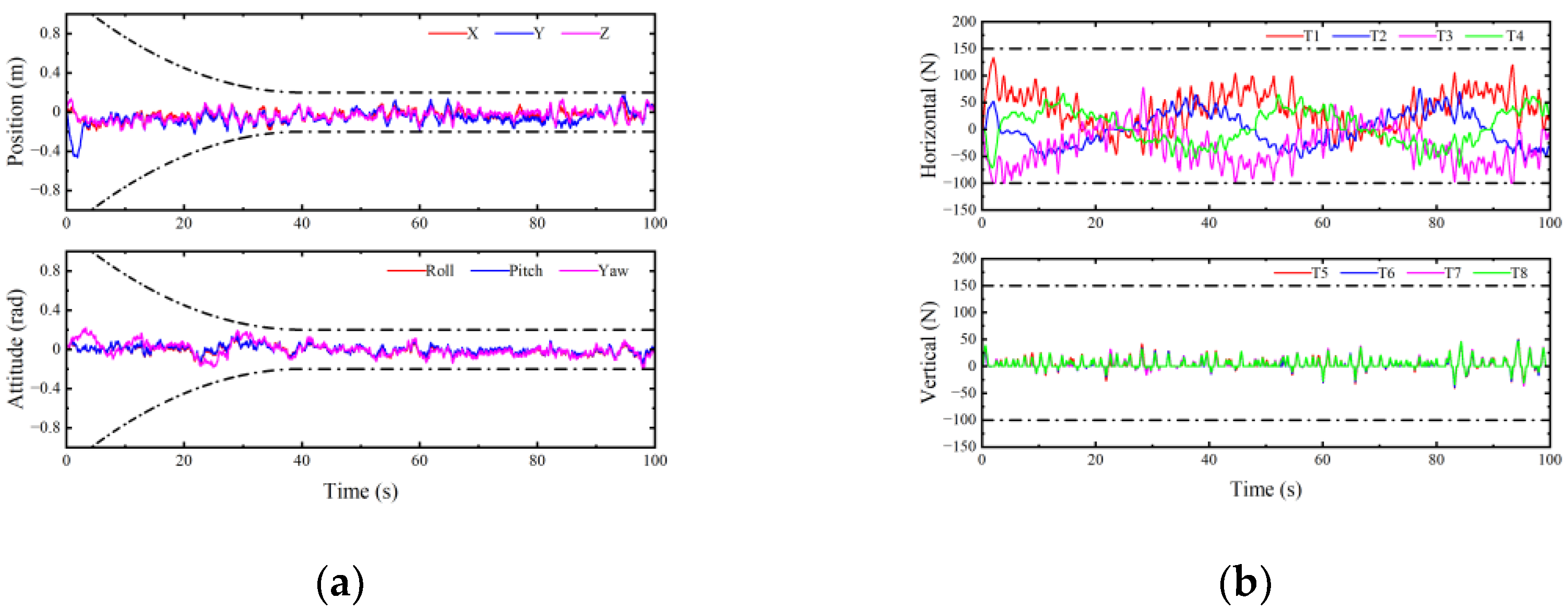
4.2. Experimental Results and Analysis

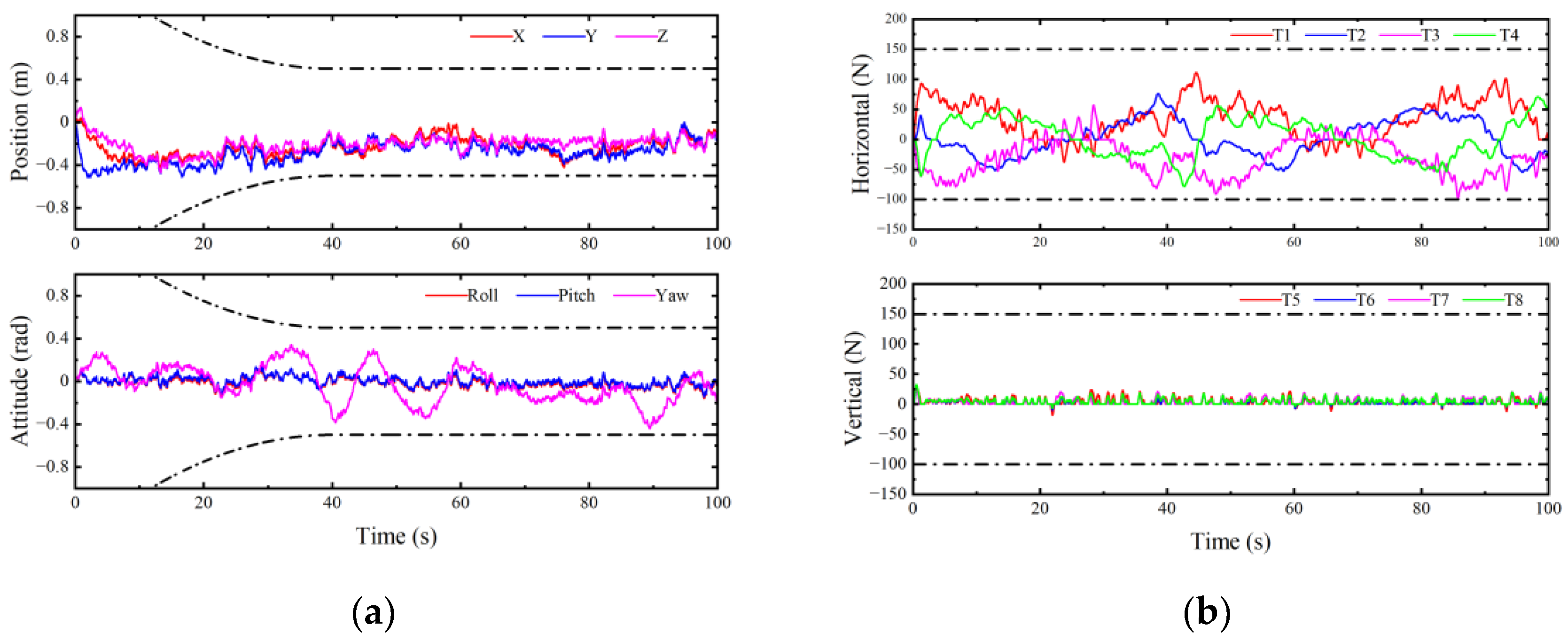
To verify the performance of the AUV finite-time region tracking control method based on command filter in terms of control signal smoothing and energy consumption, the following two cases were considered, and the experimental results in these two cases are analyzed below.

Case 1 [31]: A performance function with a large range is set, and the parameters of the performance function (Equation (3)) in this paper are $\rho (T)=0.5$—which is the final convergence range— $\rho (0)=1+\rho (T)$, $T=40$, $q_1=1$, and $q_2=2$.

Case 2 [31]: A performance function with a large range is set, and the parameters of the performance function (Equation (3)) in this paper are: $\rho (T)=0.2$—which is the final convergence range—, $\rho (0)=1+\rho (T)$, $T=40$, $q_1=1$ and, $q_2=2$.

(1)

Experimental results and analysis in case 1

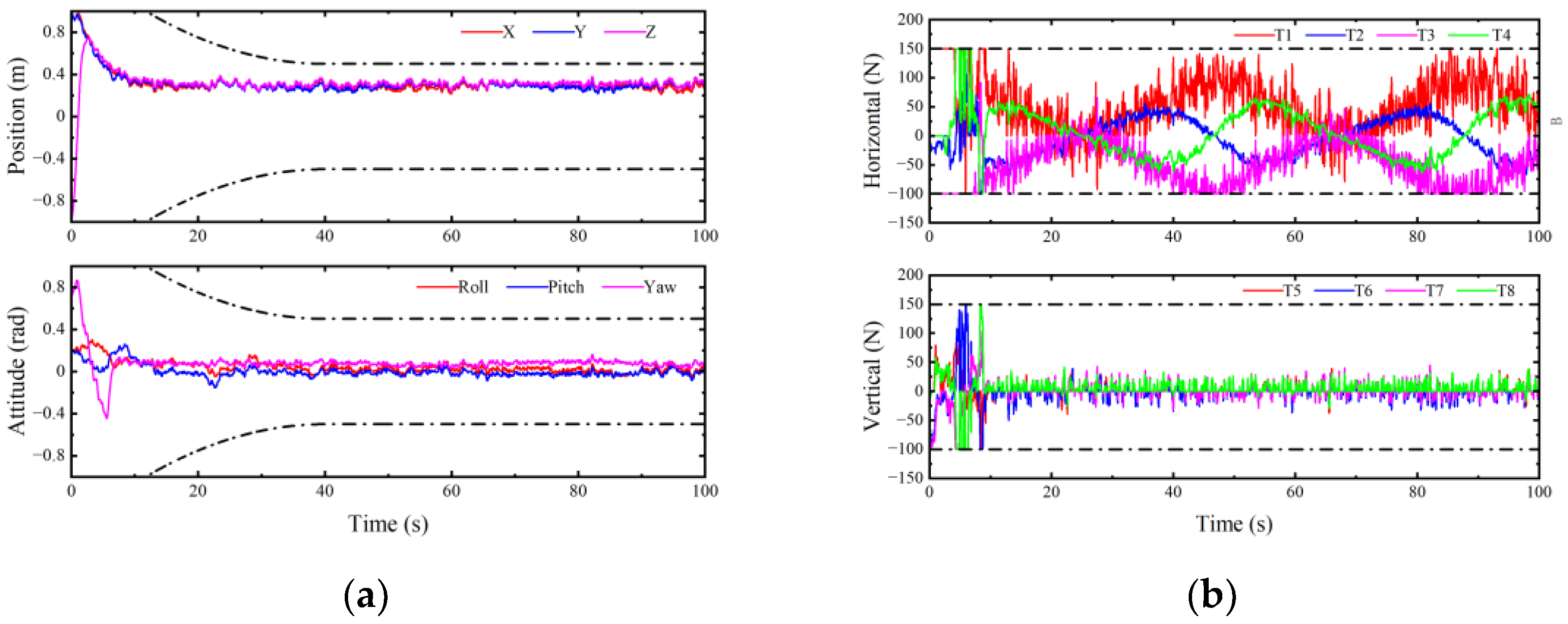
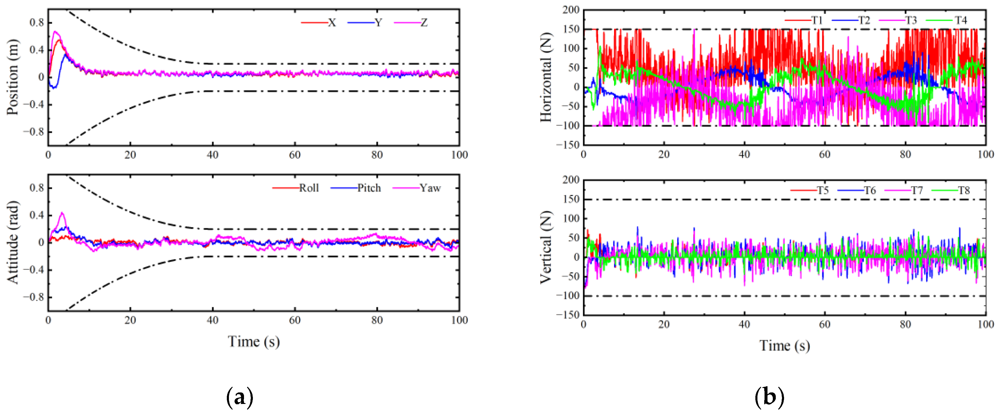
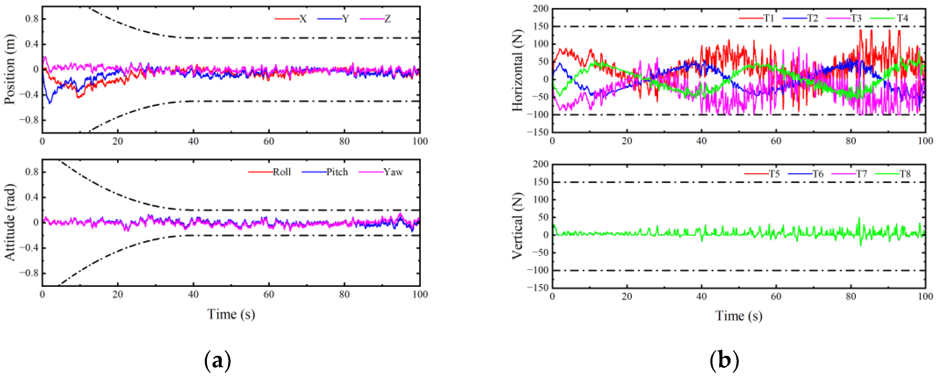
Since case 1 has a lower requirement for AUV constraints, the controller can appropriately select smaller parameters to reduce the response speed of the controller in exchange for smoother control signals. The parameters in this paper are as follows: the allowable error is set as ${\vartheta }_{ti}=0.2$; error transformation coefficient is set as $\epsilon =0.2$; the parameter in the filter is set as $r_3=5$, $r_4=10$, $r_5=1$, $r_6=10$; the parameters of controller and compensator are set as $k_1=1.2$, $k_2=3$, $k_v=1$, $k_{\tau }=1$; and other parameters are $P=1/3$ and $\omega =0.1$. In Case 1, the tracking errors and control signals of the proposed method and the methods in [28,31] are shown in Figure 3, Figure 4 and Figure 5.

In Figure 3, Figure 4 and Figure 5, X, Y, and Z, roll, pitch, and yaw represent the position error and attitude error of ODIN AUV in the geodetic coordinate system. T1–T4 and T5–T8 are respectively used for the control signals of ODIN AUV horizontal and vertical thrusters. The chain lines in Figure 3a, Figure 4a, and Figure 5a indicate the range of performance function constraints. The chain lines in Figure 3b, Figure 4b, and Figure 5b indicate the saturation value of the control signal.

As shown as From Figure 3a, Figure 4a, and Figure 5a, both the proposed method and the comparison method can keep the tracking error within the specified range of performance function; that is, the constraint requirements for the transient and steady-state performance of AUV are met. At the same time, the results show that the tracking error of the proposed method does not converge to zero, which satisfies the design objective of region tracking and conforms to the theoretical analysis in this paper. As shown in Figure 3b, Figure 4b, and Figure 5b, the proposed method is significantly different from the comparison method in terms of control signals with regard to satisfying regional tracking and performance constraints. From the overall trend, the change rules of the control signals of the three methods are similar. However, when observing the details for the control signals, it is found that the control signals in [28] show high frequency and large amplitude fluctuations, while those in this paper and in [31] are smoother.

In order to quantitatively analyze the effect of the method presented in Case 1, data in Figure 3b, Figure 4b, and Figure 5b were extracted to compare the performance of the three methods in terms of control signal smoothness and energy consumption, and

Table 1. Performance of control signals between the proposed method and the traditional method in Case 1.

	SCIS (N)									SSCS (107 × N2)
	T1	T2	T3	T4	T5	T6	T7	T8	Total
This paper	2546	1244	2695	1466	1932	1546	1414	1778	14,621	6.41
[28]	30,522	7107	18,611	5532	7202	9463	9319	8220	95,976	12.92
[31]	6737	2887	6680	2932	1877	1918	1938	1902	26,871	6.13

reports the results. Among them, the smoothness evaluation index of control signal and the evaluation index of energy consumption were selected and compared to [28,31] using the same method, specifically:

Control signal smoothness evaluation index (SCIS): $SCIS={\displaystyle \sum \Delta u_s}$, where $\Delta u_s$ represents the difference between the current and previous time of the control signal. Energy consumption evaluation indexes (SSCS): $SSCS={\displaystyle \sum {\displaystyle \sum _{i=1}^8|u_s{|}^2}}$.

The content in Table 1 was analyzed and compared. Compared to the method in [28], the smoothness index of control signals of each propeller decreased by: 91.66%, 82.50%, 85.52%, 73.50%, 71.17%, 83.66%, 84.83%, and 78.37%; total smoothness decreased by 84.77%, and energy consumption decreased by 50.39%; compared to the methods in [31], the smoothness indexes of control signals of each propeller were reduced by 62.21%, 56.91%, 59.66%, 50.00%, −2.93%, 19.40%, 27.04% and 6.52%; total smoothness was reduced by 45.59%; and energy consumption was increased by 4.57%. From the data analysis, compared with [28,31], the method presented in this paper significantly improved the smoothness of control signals. Since the adopted tracking trajectory is mainly plane motion, the performance is more obvious with horizontal thrusters (T1–T4). Compared with the method in [28], the energy consumption increases when using the method in this paper is also obvious, but it is slightly higher than that in [31]. Considering the actual work of AUV propeller, constantly changing control signals will also cause energy consumption loss, and compared with the control signal adjustment and smoothness index, the increased low energy consumption index is reasonable and acceptable.

(2)

Experimental results and analysis of case 2

As a performance function with stronger constraint ability is selected in case 2, some parameters need to be adjusted to improve the control ability of the controller to control AUV compared with case 1. Therefore, the following parameters were modified: the set value of allowable error ${\vartheta }_{ti}=0.1$ was reduced, the error transformation coefficient $\epsilon =0.4$ is increased, and the control gains $k_1=1.5$ and $k_2=5$ were increased, while other parameters remain unchanged. Based on the above parameter adjustment, in Case 2, the tracking error and control signal of the proposed method and those in [28,31] are shown in Figure 6.

The lines in Figure 6, Figure 7 and Figure 8 represent the same meanings as those in Figure 3, Figure 4 and Figure 5. It can be seen from Figure 6a, Figure 7a, and Figure 8a that the tracking errors with the proposed method and the comparison method are always within the specified range of performance function, which meets the constraint requirements on the transient and steady-state performance of AUVs. Meanwhile, it can be observed that the tracking errors with the proposed method still do not converge to zero. According to Figure 6b, Figure 7b, and Figure 8b, in case 2, the fluctuation of control signals with the three methods is roughly the same as that in case 1; that is, the control signals presented in [28] show relatively drastic fluctuations, and those in the proposed method and the method in [31] show smoother control curves than the method in [28]. To quantitatively analyze the effect of the method presented in Case 2, the data in Figure 6b, Figure 7b, and Figure 8b were extracted to compare the performance of the three methods in terms of control signal smoothness and energy consumption, and

Table 2. Performance of control signals between the proposed method and the traditional method in Case 2.

	SCIS (N)									SSCS (107 × N2)
	T1	T2	T3	T4	T5	T6	T7	T8	Total
This paper	5089	2305	5261	2301	3140	2937	2794	3012	26,839	7.05
[28]	50,970	6857	38,130	9365	12,694	21,701	19,615	11,102	170,434	13.87
[31]	15,216	4871	14,742	4877	3761	3916	38,483	3794	55,025	7.15

reports the results.

The content of Table 2 was analyzed and compared. Compared to [28], the smoothness index of control signals of each propeller decreased 90.02%, 66.38%, 86.20%, 75.43%, 75.26%, 86.47%, 85.76%, 72.87%, and 49.17%; the total smoothness decreased by 84.25%; and energy consumption decreased by 49.17%. Compared to the [31], the smoothness indexes of control signals of each propeller are reduced by 66.55%, 52.68%, 64.31%, 52.82%, 16.51%, 25.00%, 27.39%, and 20.61%; the total smoothness was reduced by 51.22%; and energy consumption was reduced by 1.40%. According to the data analysis, compared [28,31], the method in this paper significantly improved the smoothness of the control signal, and reduced the energy consumption to varying degrees. This shows the effectiveness of this method in smoothing control signal and reducing energy consumption.

In general, based on the method presented in this paper and the simulation results of [28,31] in Case 1 and Case 2, it is verified that the proposed AUV finite-time region-tracking control method based on command filter can ensure that the AUV tracking error meets the transient and steady-state constraints and does not have to converge to zero. An analysis of the three methods in terms of the control signal smoothness and energy consumption indices shows that the method in this paper has the advantage of control signal smoothness and at the same time maintains the reduced energy consumption achieved in [31].

If the method in the paper is used in practical implementation, it is necessary to jointly adjust the allowable error range and the command filter parameters based on the actual working environment and safety requirements. Since this paper does not design a dynamic parameter adjustment link, if the method is applied in harsh underwater environments, a more conservative allowable error range needs to be selected. If the method is applied to formation control, the influence of other agents should also be considered [49].

5. Conclusions

In this paper, the AUV region tracking control problem with measurement noise and transient and steady-state constraints is studied, and a commandfilter-based region-tracking control method for AUV with measurement noise is proposed. An improved nonlinear tracking error transformation method is proposed to realize the tracking error of AUV in a relatively simple way to meet the performance constraints and regional tracking requirements. At the same time, a method based on second-stage command filter is proposed to reduce the influence of measurement noise on the control signal. Based on the proposed method, a closed-loop system is designed. The results of the closed-loop system stability analysis show that the proposed method can realize finite-time convergence of tracking errors to a set allowable error boundary, even in the presence of measurement noise, unknown current, and thruster fault. Simulation experiment results based on ODIN AUV show that the tracking error under the proposed method meets the requirements of performance constraints and regional tracking, and the smoothness index of control signals increases by 84.50% and 48.40% on average compared with the method in [28]. The energy consumption index is reduced by an average of 50.81% compared to the method in [28] and increased by an average of 1.59% compared to the method in [31]. The simulation results show the advantages of the proposed method in smoothing control signals, but the performance in reducing energy consumption is slightly inferior to that of the method in [31] and needs to be improved. The simulation results show that the proposed method is suitable for a class of AUV tasks that have loose and fixed accuracy requirements and require safe and stable operation over a wide range and long endurance, such as marine resource exploration and search for wreckage of crashed aircraft.

Research prospects: In order to further reduce the conservatism of the proposed method, further research is needed to investigate how to maintain the AUV to track the region under performance constraints when the upper bound of the disturbance is unknown. In addition, considering the large inertial characteristics of the AUV, the time series state information of the AUV and the desired trajectory in future can be incorporated into the proposed method to further reduce energy consumption, which will have a positive effect on improving the working time of one action. As a research trend, it can be attempted to apply the proposed method to multi-agent formation [50].

References

1. Tabataba’i-Nasab, F.S.; Khalaji, A.K.; Moosavian, S.A.A. Adaptive nonlinear control of an autonomous underwater vehicle. Trans. Inst. Meas. Control 2019, 41, 3121–3131. [Google Scholar] [CrossRef]
2. Zereik, E.; Bibuli, M.; Mišković, N.; Ridao, P.; Pascoal, A. Challenges and future trends in marine robotics. Annu. Rev. Control 2018, 46, 350–368. [Google Scholar] [CrossRef]
3. Guerrero, J.; Torres, J.; Creuze, V.; Chemori, A. Trajectory tracking for autonomous underwater vehicle: An adaptive approach. Ocean Eng. 2019, 172, 511–522. [Google Scholar] [CrossRef]
4. Xiao, B.; Yang, X.; Karimi, H.R.; Qiu, J. Asymptotic Tracking Control for a More Representative Class of Uncertain Nonlinear Systems with Mismatched Uncertainties. IEEE Trans. Ind. Electron. 2019, 66, 9417–9427. [Google Scholar] [CrossRef]
5. Dai, Y.; Yu, S.; Yan, Y.; Yu, X. An EKF-Based Fast Tube MPC Scheme for Moving Target Tracking of a Redundant Underwater Vehicle-Manipulator System. IEEE ASME Trans. Mechatron. 2019, 24, 2803–2814. [Google Scholar] [CrossRef]
6. Sun, W.; Su, S.F.; Wu, Y.; Xia, J.; Nguyen, V.T. Adaptive Fuzzy Control with High-Order Barrier Lyapunov Functions for High-Order Uncertain Nonlinear Systems with Full-State Constraints. IEEE Trans. Cybern. 2020, 50, 3424–3432. [Google Scholar] [CrossRef]
7. Cui, R.; Chen, L.; Yang, C.; Chen, M. Extended State Observer-Based Integral Sliding Mode Control for an Underwater Robot with Unknown Disturbances and Uncertain Nonlinearities. IEEE Trans. Ind. Electron. 2017, 64, 6785–6795. [Google Scholar] [CrossRef]
8. Chengzhi, Y.; Licht, S.; Haibo, H. Formation Learning Control of Multiple Autonomous Underwater Vehicles with Heterogeneous Nonlinear Uncertain Dynamics. IEEE Trans. Cybern. 2018, 48, 2920–2934. [Google Scholar] [CrossRef]
9. Wang, H.; Pan, Y.; Li, S.; Yu, H. Robust Sliding Mode Control for Robots Driven by Compliant Actuators. IEEE Trans. Control. Syst. Technol. 2019, 27, 1259–1266. [Google Scholar] [CrossRef]
10. Cheah, C.C.; Sun, Y.C. adaptive-region-control-for-autonomous-underwater-vehicles.pdf. In Proceedings of the Oceans ‘04 MTS/IEEE Techno-Ocean ‘04 Conference, Kobe, Japan, 9–12 November 2004. [Google Scholar]
11. Ismail, Z.H.; Faudzi, A.A.; Dunnigan, M.W. Fault-Tolerant Region-Based Control of an Underwater Vehicle with Kinematically Redundant Thrusters. Math. Probl. Eng. 2014, 2014, 527315. [Google Scholar] [CrossRef]
12. Sun, X.; Ge, S.S. A DSC approach to adaptive dynamic region-based tracking control for strict-feedback non-linear systems. IET Control. Theory Appl. 2021, 16, 94–111. [Google Scholar] [CrossRef]
13. Liu, X.; Zhang, M. Region tracking control for autonomous underwater vehicle with control input saturation. In Proceedings of the 39th Chinese Control Conference (CCC), Shenyang, China, 27 July 2020; pp. 2615–2620. [Google Scholar]
14. Parisa, S.; Sani, S.K.H. Barrier Lyapunov functions-based adaptive neural tracking control for non-strict feedback stochastic nonlinear systems with full-state constraints: A command filter approach. Math. Control Relat. Fields 2023, 13, 988–1007. [Google Scholar]
15. Liu, J. Converse Barrier Functions via Lyapunov Functions. IEEE Trans. Autom. Control 2022, 67, 497–503. [Google Scholar] [CrossRef]
16. Liu, L.; Liu, Y.-J.; Chen, A.; Tong, S.; Chen, C.L.P. Integral Barrier Lyapunov function-based adaptive control for switched nonlinear systems. Sci. China Inf. Sci. 2020, 63, 132203. [Google Scholar] [CrossRef]
17. Liu, C.; Wang, H.; Liu, X.; Zhou, Y. Adaptive Finite-Time Fuzzy Funnel Control for Nonaffine Nonlinear Systems. IEEE Trans. Syst. Man Cybern. Syst. 2021, 51, 2894–2903. [Google Scholar] [CrossRef]
18. Hu, J.; Trenn, S.; Zhu, X. Funnel Control for Relative Degree One Nonlinear Systems with Input Saturation. In Proceedings of the 2022 European Control Conference (ECC), London, UK, 11–14 July 2022; pp. 227–232. [Google Scholar]
19. Wang, S.; Yu, H.; Yu, J.; Na, J.; Ren, X. Neural-Network-Based Adaptive Funnel Control for Servo Mechanisms with Unknown Dead-Zone. IEEE Trans Cybern 2020, 50, 1383–1394. [Google Scholar] [CrossRef]
20. Li, J.; Tian, Z.Y.; Zhang, H.H.; Li, W.B. Robust Finite-Time Control of a Multi-AUV Formation Based on Prescribed Performance. J. Mar. Sci. Eng. 2003, 11, 897. [Google Scholar] [CrossRef]
21. Elhaki, O.; Shojaei, K. Neural network-based target tracking control of underactuated autonomous underwater vehicles with a prescribed performance. Ocean. Eng. 2018, 167, 239–256. [Google Scholar] [CrossRef]
22. Li, J.; Du, J.; Sun, Y.; Lewis, F.L. Robust adaptive trajectory tracking control of underactuated autonomous underwater vehicles with prescribed performance. Int. J. Robust Nonlinear Control 2019, 29, 4629–4643. [Google Scholar] [CrossRef]
23. Qin, H.; Wu, Z.; Sun, Y.; Zhang, C.; Lin, C. Fault-Tolerant Prescribed Performance Control Algorithm for Underwater Acoustic Sensor Network Nodes with Thruster Saturation. IEEE Access 2019, 7, 69504–69515. [Google Scholar] [CrossRef]
24. Liu, H.; Meng, B.; Tian, X. Finite-Time Prescribed Performance Trajectory Tracking Control for Underactuated Autonomous Underwater Vehicles Based on a Tan-Type Barrier Lyapunov Function. IEEE Access 2022, 10, 53664–53675. [Google Scholar] [CrossRef]
25. Zhou, C.; Dai, C.; Yang, J.; Li, S. Disturbance observer-based tracking control with prescribed performance specifications for a class of nonlinear systems subject to mismatched disturbances. Asian J. Control 2023, 25, 359–370. [Google Scholar] [CrossRef]
26. Wang, Y.; Su, B.; Guo, B. Finite time state tracking control based on prescribed performance for a class of constrained nonlinear systems. Int. J. Robust Nonlinear Control 2023, 33, 7114–7129. [Google Scholar] [CrossRef]
27. Li, J.; Du, J.; Chen, C.L.P. Command-Filtered Robust Adaptive NN Control with the Prescribed Performance for the 3-D Trajectory Tracking of Underactuated AUVs. IEEE Trans. Neural Netw. Learn. Syst. 2022, 33, 6545–6557. [Google Scholar] [CrossRef] [PubMed]
28. Liu, X.; Zhang, M.; Wang, S. Adaptive region tracking control with prescribed transient performance for autonomous underwater vehicle with thruster fault. Ocean Eng. 2020, 196, 106804. [Google Scholar] [CrossRef]
29. Pagliai, M.; Ridolfi, A.; Gelli, J. Design of a Reconfigurable Autonomous Underwater Vehicle for Offshore Platform Monitoring and Intervention. In Proceedings of the IEEE/OES Autonomous Underwater Vehicle Workshop, Porto, Portugal, 6–9 November 2018. [Google Scholar]
30. Le, K.; To, A.; Leighton, B. The SPIR: An AUR for Bridge Pile Cleaning and Condition Assessment. In Proceedings of the IEEE/RSJ International Coference on Intelligant Robots and Systems (IROS), Las Vegas, NV, USA, 24 October 2020–24 January 2021. [Google Scholar]
31. Liu, X.; Zhang, M.; Yao, F.; Yin, B.; Chen, J. Barrier Lyapunov function based adaptive region tracking control for underwater vehicles with thruster saturation and dead zone. J. Frankl. Inst. 2021, 358, 5820–5844. [Google Scholar] [CrossRef]
32. Farrell, J.A.; Polycarpou, M.; Sharma, M.; Dong, W. Command Filtered Backstepping. In Proceedings of the 2008 American Control Conference, Seattle, WA, USA, 11–13 June 2008; Volume 1–12, pp. 1391–1395. [Google Scholar]
33. Yu, J.; Shi, P.; Zhao, L. Finite-time command filtered backstepping control for a class of nonlinear systems. Automatica 2018, 92, 173–180. [Google Scholar] [CrossRef]
34. Li, C.; Zhang, Y.; Li, P. Full control of a quadrotor using parameter-scheduled backstepping method: Implementation and experimental tests. Nonlinear Dyn. 2017, 89, 1259–1278. [Google Scholar] [CrossRef]
35. Yu, J.; Zhao, L.; Yu, H.; Lin, C.; Dong, W. Fuzzy Finite-Time Command Filtered Control of Nonlinear Systems with Input Saturation. IEEE Trans. Cybern. 2018, 48, 2378–2387. [Google Scholar] [CrossRef]
36. Gao, Y.; Li, C.; Li, D. Command Filter-Based Control for Spacecraft Attitude Tracking with Pre-Defined Maximum Settling Time Guaranteed. IEEE Access 2021, 9, 69663–69679. [Google Scholar] [CrossRef]
37. Wang, H.; Kang, S.; Zhao, X.; Xu, N.; Li, T. Command Filter-Based Adaptive Neural Control Design for Nonstrict-Feedback Nonlinear Systems with Multiple Actuator Constraints. IEEE Trans. Cybern. 2022, 52, 12561–12570. [Google Scholar] [CrossRef] [PubMed]
38. Qiu, J.; Sun, K.; Rudas, I.J.; Gao, H. Command Filter-Based Adaptive NN Control for MIMO Nonlinear Systems with Full-State Constraints and Actuator Hysteresis. IEEE Trans. Cybern. 2020, 50, 2905–2915. [Google Scholar] [CrossRef] [PubMed]
39. Liu, Q.; Li, M. Discrete-Time Position Control for Autonomous Underwater Vehicle under Noisy Conditions. Appl. Sci. 2021, 11, 5790. [Google Scholar] [CrossRef]
40. Wang, Q.; Liu, K.; Cao, Z. System noise variance matrix adaptive Kalman filter method for AUV INS/DVL navigation system. Ocean Eng. 2023, 267, 113269. [Google Scholar] [CrossRef]
41. Qiao, L.; Zhang, W. Adaptive Two-stage Fast Nonsingular Terminal Sliding Mode Tracking Control for Fully Actuated Autonomous Underwater Vehicles. IEEE J. Ocean Eng. 2019, 44, 363–385. [Google Scholar] [CrossRef]
42. Qiao, L.; Zhang, W. Double-Loop Integral Terminal Sliding Mode Tracking Control for UUVs with Adaptive Dynamic Compensation of Uncertainties and Disturbances. IEEE J. Ocean Eng. 2019, 44, 29–53. [Google Scholar] [CrossRef]
43. Podder, T.K.; Sarkar, N. Fault-tolerant control of an autonomous underwater vehicle under thruster redundancy, Robot. Autom. Syst. 2001, 34, 39–52. [Google Scholar] [CrossRef]
44. Qian, C.; Lin, W. A Continuous Feedback Approach to Global Strong Stabilization of Nonlinear Systems. IEEE Trans. Autom. Control 2001, 46, 1061–1079. [Google Scholar] [CrossRef]
45. Zuo, Z.; Wang, C. Adaptive trajectory tracking control of output constrained multi-rotors systems. IET Control. Theory Appl. 2014, 8, 1163–1174. [Google Scholar] [CrossRef]
46. Zhu, Z.; Xia, Y.; Fu, M. Attitude stabilization of rigid spacecraft with finite-time convergence. Int. J. Robust Nonlinear Control 2011, 21, 686–702. [Google Scholar] [CrossRef]
47. Liu, X.; Zhang, M.; Yang, C.; Yin, B. Finite-time tracking control for autonomous underwater vehicle based on an improved non-singular terminal sliding mode manifold. Int. J. Control 2020, 95, 840–849. [Google Scholar] [CrossRef]
48. Amrr, S.M.; Nabi, M.; Tiwari, P.M. A fault-tolerant attitude tracking control of spacecraft using an anti-unwinding robust nonlinear disturbance observer. Proc. Inst. Mech. Eng. Part G–J. Aerosp. Eng. 2019, 233, 6005–6018. [Google Scholar] [CrossRef]
49. Fang, X.; Xie, L.; Li, X. Distributed localization in dynamic networks via complex Laplacian. Automatica 2023, 151, 110915. [Google Scholar] [CrossRef]
50. Fang, X.; Li, X.; Xie, L. Angle-displacement rigidity theory with application to distributed network localization. IEEE Trans. Autom. Control 2020, 66, 574–2587. [Google Scholar] [CrossRef]
Figure 1. Overall idea of AUV finite-time region tracking control method based on command filter in this paper.
Jmse 11 02119 g001
Figure 2. Design idea of traditional region tracking method in (a) [28] and (b) [31].
Jmse 11 02119 g002aJmse 11 02119 g002b
Figure 3. Tracking error and control signal of proposed method in Case 1. (a) Tracking error of the proposed method. (b) control signal of the proposed method.
Jmse 11 02119 g003
Figure 4. Tracking error and control signal of reference [28] in Case 1. (a) Tracking error of reference [28]; (b) control signal of reference [28].
Jmse 11 02119 g004
Figure 5. Tracking error and control signal of reference [31] in Case 1. (a) Tracking error of reference [31]; (b) control signal of reference [31].
Jmse 11 02119 g005
Figure 6. Tracking error and control signal of the proposed method in Case 2. (a) Tracking error of the proposed method; (b) control signal of the proposed method.
Jmse 11 02119 g006
Figure 7. Tracking error and control signal of reference [28] in Case 2. (a) Tracking error of reference [28]; (b) control signal of reference [28].
Jmse 11 02119 g007
Figure 8. Tracking error and control signal of reference [31] in Case 2. (a) Tracking error of reference [31]; (b) control signal of reference [31].
Jmse 11 02119 g008