A Deep-Sea Broadband Sound Source Depth Estimation Method Based on the Interference Structure of the Compensated Beam Output

Abstract

This paper proposes an underwater broadband target depth estimation method based on the multipath arrival structure in medium and short-range deep-sea environments. The proposed approach involves separating the multipath rays arriving at the vertical line array using the matched filtering technique. The combined beamforming is then applied to the vector hydrophone vertical array (VHVA) to obtain more accurate elevation angle estimates. The components of the interference sound field at different distances are judged, and the signal received by the array is compensated using suitable estimated angles. Finally, the multipath time delay difference is extracted from the pulse peaks of the compensated signal, and the target depth is estimated by establishing the relationship among the multipath time delay difference, the elevation angle and depth. Simulations and experiments demonstrate the effectiveness of this method in reducing the depth estimation bias and avoiding the misjudgment of surface or submerged targets.

1. Introduction

Depth estimation is a great focus in hydroacoustic passive detection. The main methods currently used for depth estimation include matched-field processing (MFP), modal filtering and multipath arrival structure-based methods. The MFP method correlates the measured sound field and the copied one to obtain the ambiguity surface. Target positioning is then achieved by searching for peak values [1,2,3,4,5,6]. However, this method is sensitive to the hydroacoustic environment and computationally intensive. Modal filtering is a method that estimates the source depth by passing the received signal through a binary mask filter. This allows for the extraction of modes of the actual sound source, which are then matched with modes of the simulated sound source [7,8,9]. However, this method requires well-sampled wave fields and is not robust. By comparison, the depth estimation method based on multipath arrival time delay or interference fringe period is simple in principle and suitable for deep sea environments.

Sound waves reach the receiving point via multiple paths, which results in time delay differences among the various paths. These time delay differences usually contain valuable information about the target depth. The most commonly used methods for extracting time delay differences rely on correlation function and multipath propagation interference properties. Duan et al. extracted the time delay difference between the direct and sea surface reflected waves by analyzing the autocorrelation function of the received signal of a single hydrophone. This method allowed them to locate the moving sound source [10]. An et al. used the cepstrum method to extract the multipath structure from the radiated noise of a sound source in a shallow sea waveguide environment. The source depth is then estimated by matched processing of multipath time delay difference [11]. Yang et al. estimated the source depth by observing that the time delay difference between surface-bottom and bottom-surface reflection reaches the minimum at the source depth [12].

The multipath time delay corresponds to the interference period in the frequency domain. The received signal can be represented as an interference structure in the frequency domain. This interference structure oscillates periodically with the propagation range and the source frequency and can be used to estimate the source depth [13]. McCargar successfully separated the depth-based signal and estimated the depth of a moving source by tracking the interference fringe of the single-frequency signal [14]. Kniffin et al. analyzed the application limitations of this method and proposed using a harmonic interference structure to enhance the accuracy [15]. Yang’s group has completed much work on depth estimation using interference structure. They tracked the interference fringe structure of the measured direct and once-sea-surface-reflected waves and then matched them with the model library to estimate the source depth [16]. Afterward, Yang transformed the oscillation period of the interference fringes into target motion velocity and depth information [17]. Their team estimated the target depth by analyzing the number of fringes [18] and made improvements to handle the situation of low signal-to-noise ratio (SNR) and weak source depth fluctuations [19]. Some scholars mapped the sound field to other domains based on the interference structure of the sound field to achieve effective separation of source depth [20,21].

The research mentioned above is focused on using either a single hydrophone or a hydrophone array. Vector hydrophones have the capability to measure both sound pressure and particle velocity simultaneously, which enables them to gather richer sound-field information and achieve higher processing gain compared to traditional hydrophones. Therefore, they have become increasingly popular in deep-sea environments in recent years. Qi et al. [22] and Li et al. [23] employed a single vector hydrophone positioned near the seafloor to obtain the arrival angle and then estimated source depth based on the interference period of the received sound intensity spectrum. According to the estimated depth, Li further performed range estimation. However, the above literature only considers short reception ranges and has high SNR requirements. There is a scarcity of literature discussing the depth estimation of weak targets at middle and short ranges.

Matched filtering (MF) is the optimal linear filter for maximizing the SNR of the output signal in a white noise environment. It is commonly used in the echo signal processing of radar and sonar [24,25]. By combining MF technology with a vector hydrophone array, the SNR requirements can be effectively reduced, providing valuable technical support for depth estimation of weak targets in the deep sea.

This paper proposes an approach that combines MF technology with the joint processing of pressure and particle velocity channels of a vector hydrophone vertical array (VHVA) to enhance the receiving SNR. Then the source depth is estimated based on the interference characteristic of the multipath structure. This algorithm significantly reduces depth estimation errors and avoids misjudgment of surface or submerged targets by reasonably selecting the interference components at different distances.

This paper is arranged as follows. Section 2 introduces the basic theory of elevation angle and depth estimation. Section 3 conducts a sound field simulation, and Section 4 performs a sea trial to verify the performance of this method. A conclusion is presented in Section 5.

2. Methods

Matched filtering technology is first applied to the signal received by VHVA to increase the SNR and separate the multipath structure. Then, rather than using the conventional beamforming of a pressure array, the sound pressure and particle velocity are processed in combination to generate more accurate target elevation angles. Afterward, the array received signal is compensated according to the interference components of the sound field, and the time delay difference between the interference components is extracted from the pulse peaks of the compensated signal. Finally, the depth estimation of the broadband source is accomplished based on the image interference effect. The algorithm proposed in our paper is named matched filtering and time delay difference extraction (MFTE). The flow diagram of the MFTE method is shown in Figure 1.

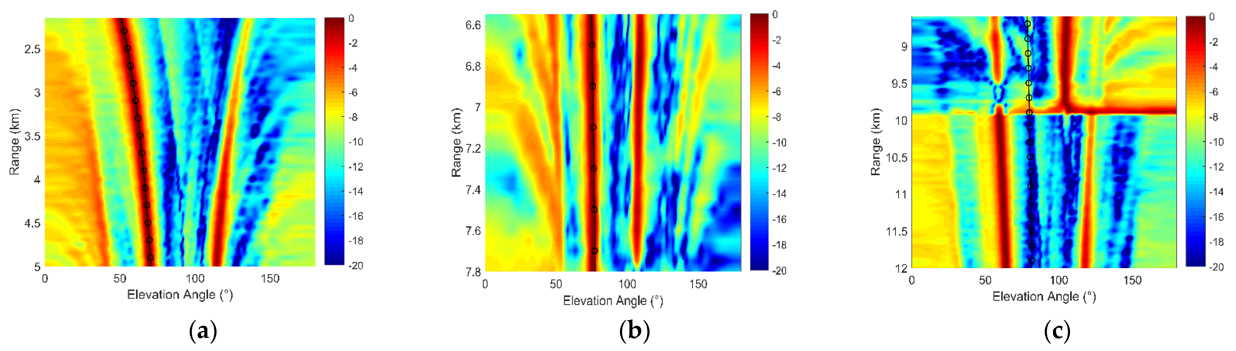
2.1. Elevation Angle Estimation

Vector hydrophones can be used to collect the sound pressure and particle velocity information underwater simultaneously. The VHVA is assumed to be composed of $M$ hydrophone elements and the element interval is $d$, as shown in Figure 2.

Suppose the sound source is placed at the elevation angle of $\phi$ and an azimuth angle of $\theta$, the signal received by VHVA can be represented as

$$X\left(t\right)=A\left(\theta ,\phi \right)S\left(t\right)+N\left(t\right)$$

(1)

where $S\left(t\right)$ and $N\left(t\right)$ represent the received signal and noise vectors, respectively. $A\left(\theta ,\phi \right)$ is the array manifold and can be expressed as

$$A\left(\theta ,\phi \right)=a\left(\theta ,\phi \right)\otimes u\left(\theta ,\phi \right)$$

(2)

where $a\left(\theta ,\phi \right)$ denotes the direction vector of the pressure array, $u\left(\theta ,\phi \right)$ is the guiding vector of a single vector hydrophone, and the symbol $\otimes$ is the Kronecker product. For the vertical line array, the propagation time difference of sound waves to each hydrophone element is decided by the elevation $\phi$ of the sound source. Thus, $u\left(\theta ,\phi \right)$ and $a\left(\theta ,\phi \right)$ can be simplified as

$$u\left(\phi \right)={\left[1,\sin \phi ,\cos \phi \right]}^T$$

(3)

$$a\left(\phi \right)={\left[1,e^{-j\frac{2\pi d\cos \phi }{\lambda }},\cdots ,e^{-j\frac{\left(M-1\right)2\pi d\cos \phi }{\lambda }}\right]}^T$$

(4)

where $\lambda$ is the wavelength corresponding to the center frequency.

Beamforming technology is often used to improve the quality of signals received by arrays in noisy environments. The conventional weight vector can be expressed as

$$w\left(\varphi \right)=A\left(\varphi \right)=a\left(\varphi \right)\otimes u\left(\varphi \right)$$

(5)

where $\varphi$ is the guiding angle. In the frequency domain, the beamforming output of the VHVA can be written as

$$Y\left(f\right)=w^H\left(\varphi \right)X\left(f\right)$$

(6)

where $X\left(f\right)$ is the Fourier transform of $X\left(t\right)$.

For pressure hydrophone vertical array (PHVA), when assuming $\phi ={\phi }_0$ and disregarding the noise, the beamforming output in the spatial power spectrum (SPS) form can be derived as

$$\begin{array}{l}P\left(\varphi \right)={\left|Y_p\left(f\right)\right|}^2={\left|w_p{}^H\left(\varphi \right)X_p\left(f\right)\right|}^2\\ \hspace{1em}\hspace{1em}={\left|\left[1,e^{j\frac{2\pi d\cos \varphi }{\lambda }},\cdots ,e^{j\frac{\left(M-1\right)2\pi d\cos \varphi }{\lambda }}\right]\cdot \left\{{\left[1,e^{-j\frac{2\pi d\cos {\phi }_0}{\lambda }},\cdots ,e^{-j\frac{\left(M-1\right)2\pi d\cos {\phi }_0}{\lambda }}\right]}^{T}S\left(f\right)\right\}\right|}^2\\ \hspace{1em}\hspace{1em}={\left|\frac{\sin \left[\left(kd\cos \varphi -kd\cos {\phi }_0\right)\cdot M/2\right]}{\sin \left[\left(kd\cos \varphi -kd\cos {\phi }_0\right)/2\right]}\right|}^2\cdot {\left|S\left(f\right)\right|}^2\end{array}$$

(7)

Similarly, the SPS of VHVA can be expressed by the following equation after derivation.

$$\begin{array}{l}{P}_v\left(\varphi \right)={\left|Y\left(f\right)\right|}^2={\left|w^H\left(\varphi \right)X\left(f\right)\right|}^2\\ \hspace{1em}\hspace{1em}={\left|\begin{array}{l}{\left[\begin{array}{ccccccc}1& \sin \varphi & \cos \varphi & \cdots & e^{-j\frac{\left(M-1\right)2\pi d\cos \varphi }{\lambda }}& e^{-j\frac{\left(M-1\right)2\pi d\cos \varphi }{\lambda }}\cdot \sin \varphi & e^{-j\frac{\left(M-1\right)2\pi d\cos \varphi }{\lambda }}\cdot \cos \varphi \end{array}\right]}^{\ast }\\ .\left\{{\left[\begin{array}{ccccccc}1& \sin {\phi }_0& \cos {\phi }_0& \cdots & e^{-j\frac{\left(M-1\right)2\pi d\cos {\phi }_0}{\lambda }}& e^{-j\frac{\left(M-1\right)2\pi d\cos {\phi }_0}{\lambda }}\cdot \sin {\phi }_0& e^{-j\frac{\left(M-1\right)2\pi d\cos {\phi }_0}{\lambda }}\cdot \cos {\phi }_0\end{array}\right]}^{T}S\left(f\right)\right\}\end{array}\right|}^2\\ \hspace{1em}\hspace{1em}={\left[1+\cos \left(\varphi -{\phi }_0\right)\right]}^2\cdot {\left|\frac{\sin \left[\left(kd\cos \varphi -kd\cos {\phi }_0\right)\cdot M/2\right]}{\sin \left[\left(kd\cos \varphi -kd\cos {\phi }_0\right)/2\right]}\right|}^2\cdot {\left|S\left(f\right)\right|}^2\end{array}$$

(8)

where ${\phi }_0$ and $k$ denote the target elevation angle and wavenumber, respectively. $S\left(f\right)$ is the Fourier transform of the transmitted signal.

For VHVA, the sound pressure and particle velocity information are often combined to obtain the higher array gain. Taking the combination of pressure $p$ and vertical particle velocity $v_z$ as an example, the SPS of $\left(p+v_z\right)\cdot v_z$ can be written as

$$\begin{array}{l}{P}_{p{v}_z}\left(\varphi \right)={\left|Y_{p{v}_z{v}_z}\left(f\right)\right|}^2=\left|Y_{p{v}_z}\left(f\right)\cdot Y_{v_z}{}^{\ast }\left(f\right)\right|\\ \hspace{1em}\hspace{1em} =\left[1+\cos \varphi \cos {\phi }_0\right]\cdot \cos \varphi \cos {\phi }_0\cdot {\left|\frac{\sin \left[\left(kd\cos \varphi -kd\cos {\phi }_0\right)\cdot M/2\right]}{\sin \left[\left(kd\cos \varphi -kd\cos {\phi }_0\right)/2\right]}\right|}^2\cdot {\left|S\left(f\right)\right|}^2\end{array}$$

(9)

For a broadband signal, it can be divided into multiple narrow bands to perform narrowband beamforming. The output of each sub-band is then spliced in the frequency domain to obtain the spatial-spectral distribution of the broadband signal. The elevation angle of the target can be estimated by searching for the maximum beam power. The elevation angle obtained is an important factor in the subsequent depth estimation.

Generally, the multipath effect in the ocean channel directly affects the elevation estimation performance of the vertical line array. MF technology can be used to distinguish the arrival structures of signals propagating through different paths. Moreover, MF technology involves coherent superposition of signals and non-coherent superposition of noise, which significantly improves the SNR of received signals. The matched filtering impulse response is written as

$$h\left(t\right)=q{s}^{\ast }\left(t_0-t\right)$$

(10)

where $q$ is the matched factor, usually set to 1. $t_0$ stands for the time delay and the symbol $\ast$ is the conjugate transpose operator.

The transfer function $H\left(f\right)$ is obtained through the Fourier transform of Equation (10), which is expressed as

$$H\left(f\right)=q{S}^{\ast }\left(f\right)e^{-2\pi f{t}_0}$$

(11)

Further, the received signal after matched filter processing can be written as

$$X_{MF}\left(f\right)=X\left(f\right)\cdot H\left(f\right)$$

(12)

Then, $X_{MF}\left(f\right)$ is substituted for $X\left(f\right)$ into Equation (6) for beamforming.

Replacing $X\left(f\right)$ by $X_{MF}\left(f\right)$ in Equation (6), the VHVA signal after time delay compensation can be expressed as

$$Y_{MF}\left(f\right)=c^H\left(\gamma \right)X_{MF}\left(f\right)\cdot e^{-j2\pi f\left(m-1\right)d\cos \gamma /c}$$

(13)

where $\gamma$ is the compensation angle and $c\left(\gamma \right)$ is the compensation vector, which equals to $w\left(\gamma \right)$ in numerical terms. Generally, the main lobe of beamforming is used as the compensation angle. However, due to the multipath effect, eigen-rays with similar amplitude and different paths arriving at the receiving array will produce two peaks with similar energy. One is the angle of upward waves and the other is that of downward waves. In some cases, the angle corresponding to the secondary maximum is applied to compensate for the signal received by the VHVA.

In general, two eigen-rays with similar amplitude and little difference in time delay constitute the eigen-ray interference structure and contribute the most to the interference field. Therefore, we only consider the case of two contributing eigen-rays interference. For example, when considering the direct (D) and once-sea-surface-reflected (S1B0) waves, the beam output functions as a spatial filter, preserving the sound energy of D and S1B0 while suppressing energy from other directions. Therefore, the SNR of the main lobe direction can be enhanced, guaranteeing the preservation of the high-energy sound field interference structure.

The beam output in the time domain $y_{MF}\left(t\right)$ can be obtained by inverse Fourier transform. Then, the time difference between the two spikes of $y_{MF}\left(t\right)$ is extracted as the time delay difference $△\tau$ between the interference eigen-rays. The processing procedure is expressed as follows

$$Y_{MF}\left(f\right)\stackrel{ifft}{\to }{y}_{MF}\left(t\right)\to △\tau$$

(14)

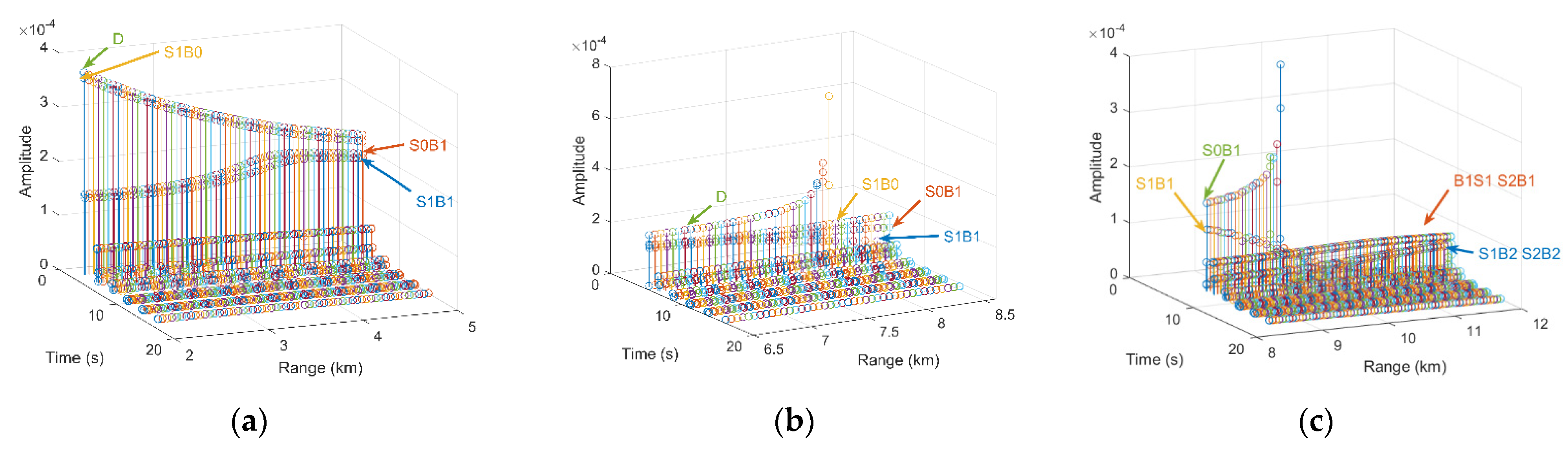
2.2. Depth Estimation

2.2.1. In the Direct Wave Zone

In the direct wave zone, the received signal is mainly contained with the components of D and S1B0 waves. The pressure signal collected at the point $\left(r,z_r\right)$ can be written as [26]

$$p(r,z_r)=\frac{1}{r_1}{e}^{ik{r}_1}-\frac{1}{r_2}{e}^{ik{r}_2}$$

(15)

where $r_1$ and $r_2$ are the propagation distance of D and S1B0. $r$ and $z_r$ represents the range and depth of the receiver. According to the geometry relation, $r_1$ and $r_2$ satisfy the relation as

$$r_1=\sqrt{r^2+{\left(z_r-z_s\right)}^2},r_2=\sqrt{r^2+{\left(z_r+z_s\right)}^2}$$

(16)

Defining $R$ as the slope distance, which satisfies the formula $R^2=r^2+z_r{}^2$. Generally speaking, the target depth is usually much less than the ocean depth. Thus, Equation (16) can be written as

$$r_1\simeq R-z_s\cos \phi ,r_2\simeq R+z_s\cos \phi$$

(17)

where $\phi =\arccos \left(z_r/R\right)$ and can be approximated by the elevation angle obtained from array beamforming. Therefore, Equation (15) can be further rewritten as

$$p(r,z_r)=\frac{e^{ikR}}{R}\cdot \left[-2i\sin \left(k{z}_s\cos \phi \right)\right]$$

(18)

The amplitude of the sound pressure is expressed as

$$\left|p(r,z_r)\right|=\frac{2}{R}\left|\sin \left(k{z}_s\cos \phi \right)\right|$$

(19)

From Equation (19) we can find that the amplitude of the pressure signal is a periodic function related to the sinusoidal modulation. The modulation period is related to the wavenumber $k$, source depth $z_s$, and elevation angle $\phi$. Let the modulation period satisfy the relation $k{z}_s\cos \phi =\pi$, the target depth can be estimated by

$$z_s=\frac{c}{2\cos \phi }\cdot △\tau$$

(20)

where $c$ is the sound speed at the receiver depth.

In theory, the particle velocity or sound energy flow of sound pressure and particle velocity can both obtain similar interference structures.

According to Euler’s formula and the relationship between the three orthogonal components of the particle velocity, each component of a single vector hydrophone can be written as

$$\left\{\begin{array}{c}p\left(t\right)=s\left(t\right)\\ v_x\left(t\right)=\frac{1}{\rho c}\cos \theta \sin \phi \cdot s\left(t\right)\\ v_y\left(t\right)=\frac{1}{\rho c}\sin \theta \sin \phi \cdot s\left(t\right)\\ v_z\left(t\right)=\frac{1}{\rho c}\cos \phi \cdot s\left(t\right)\end{array}\right.$$

(21)

Thus, another three particle velocity components at the same point are expressed as

$$\left\{\begin{array}{c}{v}_x(r,z_r)=\frac{e^{i\left(kR-\omega t\right)}}{R}\cdot \left[-2i\sin \left(k{z}_s\cos \phi \right)\right]\cdot \cos \theta \sin \phi /\rho c\\ v_y(r,z_r)=\frac{e^{i\left(kR-\omega t\right)}}{R}\cdot \left[-2i\sin \left(k{z}_s\cos \phi \right)\right]\cdot \sin \theta \sin \phi /\rho c\\ v_z(r,z_r)=\frac{e^{i\left(kR-\omega t\right)}}{R}\cdot \left[-2i\sin \left(k{z}_s\cos \phi \right)\right]\cdot \cos \phi /\rho c\end{array}\right.$$

(22)

It is discovered that the interference cycle of the particle velocity signal’s modulus is not only dependent on $\sin \left(k{z}_s\cos \phi \right)$ but also on the natural directivity of particle velocity components. Therefore, we eliminate the impact of dipole directionality in the following manner. Firstly, the complex sound intensifier method is used for the VHVA to determine the azimuth angle of the target.

$$\theta =\arctan \frac{\mathrm{Re}\left[\overline{P\cdot V_y{}^{\ast }}\right]}{\mathrm{Re}\left[\overline{P\cdot V_x{}^{\ast }}\right]}$$

(23)

Then the horizontal particle velocity can be constructed as follows

$$\begin{array}{l}{v}_r=v_x\cdot \cos {\theta }_0+v_y\cdot \sin {\theta }_0\\ \hspace{1em}=\sin \phi \cdot \cos \left(\theta -{\theta }_0\right)\cdot p/\rho c\end{array}$$

(24)

When the guiding angle aligns with the target azimuth, the above equation can be simplified as $v_r=\sin \phi \cdot p/\rho c$. Combined beamforming is used for the VHVA to achieve elevation angle estimation. Then the particle velocity $v$ can be written as

$$\begin{array}{l}v=v_r\cdot \sin {\phi }_0+v_z\cdot \cos {\phi }_0\\ =\sin \left(\phi -{\phi }_0\right)\cdot p/\rho c\end{array}$$

(25)

When the guiding angle $\phi$ aligns with the elevation angle, the above equation can be simplified as $v(r,z_r)=p(r,z_r)/\rho c$. The construction of particle velocity can eliminate the influence of the amplitude from different channels of VHVA. Furthermore, $\left|v(r,z_r)\right|$ has the same oscillation period as the $\left|p(r,z_r)\right|$, with a period of $△F=\frac{c}{2z_s\cos \phi }$.

Similarly, sound energy flow of sound pressure and particle velocity can form the interference structure, which can be expressed as

$$I_v=p(r,z_r)\cdot v^{\ast }(r,z_r)={\left|p(r,z_r)\right|}^2/\rho c$$

(26)

Substituting Equation (19) into Equation (26), Equation (26) can be further simplified as follows

$$I_v=\frac{4{\sin }^2\left(k{z}_s\cos \theta \right)}{\rho c{R}^2}=\frac{2}{\rho c{R}^2}\left[1-\cos \left(2k{z}_s\cos \theta \right)\right]$$

(27)

The interference cycle is $△F^{\text{'}}=\frac{c}{2z_s\cos \phi }$, which is consistent with the interference period of $\left|p(r,z_r)\right|$.

Thus, the sound pressure, particle velocity and the sound energy flow can form the same interference structure.

2.2.2. Outside the Direct Wave Zone

As illustrated in Section 2.2.1, the sound pressure and particle velocity can form a consistent interference structure. Thus, this section takes the particle velocity interference as an example to derive the expression of target depth.

For the range beyond the direct wave zone, the sound field consists mainly of once-sea-bottom-reflected (S0B1), once-sea-surface and once-sea-bottom-reflected (S1B1), once-sea-surface-reflected (B1S1) and twice-sea-surface and once-sea-bottom-reflected (S2B1) waves. These four propagation distances can be expressed as follows

$$r_{\mathrm{S}0\mathrm{B}1}=\sqrt{r^2+{\left(2H-z_r-z_s\right)}^2}$$

(28)

$$r_{\mathrm{S}1\mathrm{B}1}=\sqrt{r^2+{\left(2H-z_r+z_s\right)}^2}$$

(29)

$$r_{\mathrm{B}1\mathrm{S}1}=\sqrt{r^2+{\left(2H+z_r-z_s\right)}^2}$$

(30)

$$r_{\mathrm{S}2\mathrm{B}1}=\sqrt{r^2+{\left(2H+z_r+z_s\right)}^2}$$

(31)

where $H$ is the ocean depth.

For the interference structure composed of S0B1 and S1B1, the particle velocity signal can be expressed as follows

$$v(r,z_r)=\frac{e^{ik\sqrt{\epsilon }}}{\sqrt{\epsilon }}\cdot \left\{-2i\sin \left[k{z}_s\left(\frac{2H-z_r}{\sqrt{\epsilon }}\right)\right]\right\}/\rho c$$

(32)

where $\epsilon$ satisfies the relation $\epsilon =R^2+4H^2-4H{z}_r$.

The horizontal range $r$ of the target source can be estimated approximately according to the formula $r_{est}\approx \tan \phi .\left(2H-z_r\right)$. Therefore, the slope distance can be further written as $R_{est}{}^2=r_{est}{}^2+z_r{}^2$.

Considering the case that the interference structure is formed by the superposition of B1S1 and S2B1, the particle velocity signal can be written as

$$v(r,z_r)=\frac{e^{ik\sqrt{\chi }}}{\sqrt{\chi }}\cdot \left\{-2i\sin \left[k{z}_s\left(\frac{z_r+2H}{\sqrt{\chi }}\right)\right]\right\}/\rho c$$

(33)

where $\chi$ satisfies the formula $\chi =R^2+4H^2+4H{z}_r$. Similarly, the slope distance can be estimated according to the formula $R_{est}\approx {\left[\tan \phi .\left(2H+z_r\right)\right]}^2+z_r{}^2$.

Similar to the situation in the direct wave zone, the oscillation period of the interference structure in Equations (32) and (33) is set to be $\pi$, and the corresponding depth estimation expression is written as follows

$$z_{\mathrm{S}0\mathrm{B}1-\mathrm{S}1\mathrm{B}1}=\frac{c\sqrt{\epsilon }}{2\left(2H-z_r\right)}\cdot △\tau$$

(34)

$$z_{\mathrm{B}1\mathrm{S}1-\mathrm{S}2\mathrm{B}1}=\frac{c\sqrt{\chi }}{2\left(2H+z_r\right)}\cdot △\tau$$

(35)

3. Simulation

Bellhop is a commonly used model for analyzing sound propagation underwater based on ray theory. This section simulates the arrival structure of eigen-rays by the Bellhop model. The SSP used in the simulation shows a non-full deep-sea channel, as presented in Figure 3. The ocean depth is 2000 m, and the sound speed reaches its minimum value at approximately 960 m. The sea floor is flat, and the main seabed parameters, such as sound speed, density and sound absorption coefficient are based on the empirical values.

In addition to the above environment parameters, other vital parameters of the sound source and array are listed in

Table 1. Parameters set in simulation.

Parameter	Value
Source depth	50 m
Source form	30–500 Hz LFM
SNR	0 dB
Signal duration	1 s
Sampling rate	16 kHz
Element number	8
Element interval	7.5 m
Array depth	1750–1802.5 m

. A schematic diagram of the sound source and array positions in the simulation is shown in Figure 4.

In the simulation, the sound source radiates the LFM signal with a frequency band of 30–500 Hz. The noise is assumed to be Gaussian white type, and the SNR is set to 0 dB. Horizontal ranges between the source and receiver are set at 2.1 km to 5 km, 6.5 km to 7.8 km and 8.6 km to 12 km, respectively, involving three typical types of interference structure.

Figure 5 shows the signal received by the 8th hydrophone at the horizontal range of 3.5 km, 7 km, and 11.5 km, respectively. From Figure 5 we can find that the eigen-ray components of different propagation paths can be separated in the time domain after MF processing. Two wave packets can be observed, and the spikes in each wave packet represent the sound wave components with higher energy. Note that in Figure 5c, the amplitude of the first arrival eigen-ray at 11.5 km is negative. That is because B1S1 arrives prior to S0B1 and the amplitude of B1S1 is negative.

For the VHVA, the combined beamforming with the form of $\left(p+v_z\right)\cdot v_z$ is applied to obtain the elevation angle of the sound source. The estimated elevation angle with range is shown in Figure 6, in which the black line with circles denotes the elevation angle corresponding to the direct wave. Note that this paper defines the angle between the propagation path and the upward axis of the vertical array as the elevation angle. Therefore, the angle of the downward wave ranges from 0° to 89°, and the angle of the upward wave ranges from 91° to 180°. 90° represents the abeam direction of the vertical array.

In Figure 6a, there are two main distinct elevation angle tracks, of which the one varying from about 50° to 70° is more dominant and agrees well with the black line. This is because when the horizontal range is 2.1–5 km, the receivers are within the direct-wave zone and the dominant sound components are D and S1B0.

As the horizontal range of the source increases to 6.5–7.8 km, the eigen-rays reflected from the seabed become even more important. As shown in Figure 6b, the peak near about 110° becomes more apparent. Further, when the horizontal range of the source increases to 8.6–10 km, the direct sound wave disappears. When the horizontal range is greater than 10 km, the main lobe is about 60° and the secondary maximum appears at 115°. It is indicated that the sound energy in this case is mainly composed of multiple reflected sound waves from the seabed.

Figure 7 presents the arrival structure of eigen-rays for the 8th hydrophone at three different horizontal ranges, which further interprets the energy distribution of the beam at different angles.

In Figure 7a, amplitudes of D and S1B0 are significantly higher than those of other paths, and the corresponding amplitude difference is getting lower with the range increasing. As shown in Figure 7b, the amplitudes of D and S1B0 decrease and gradually approach those of S0B1 and S1B1. Thus, the energy of the secondary maximum in Figure 6b is nearly as high as that of the main lobe. It is well known that eigen-rays with similar amplitudes can form interference structures with equally spaced light and dark fringes. However, the amplitude difference between D and S1B0 is higher than that between S0B1 and S1B1. Therefore, S0B1 and S1B1 in the second case are two main components that form the interference structure, and the time delays of the signal received by VHVA should be compensated according to the arrival angles of S0B1 and S1B1 in the beamforming process. In the third case, S0B1 and S1B1 have even higher energy when the horizontal range is from 8.6 km to about 10 km, but the amplitude difference between the two gradually increases with distance. As the range continues to increase, S0B1 and S1B1 disappear, and B1S1 and S2B1 become more dominant.

In this paper, the arrival angles of D and S0B1 are used as compensation angles in the beamforming process for these short distances. In the middle ranges, time delays of the signal received by the array will be compensated with the arrival angles of S0B1 and S1B1. When the horizontal range reaches more than 8.6 km, the arrival angles of B1S1 and S2B1 are regarded as the compensation angles.

According to the compensation method described, signals received from each element at the range of 3.5 km, 7.0 km and 11.5 km are compensated. Figure 8 shows the received pressure signal of the 8th element before and after compensation. It is indicated that the sound field components associated with the arrival angle used in the compensation procedure are strengthened, while other sound eigen-rays are effectively suppressed. The time delay difference between two dominant eigen-rays becomes apparent, as depicted by the orange curve in Figure 8.

Further, the time delay difference of the dominant eigen-rays is extracted from two pulse peaks, and the source depths are calculated by applying the MFTE method both to a single element and the array, as shown in Figure 9 and Figure 10. Here the processing results of the 8th element of the array are selected for comparison and the depth estimation results of each element do not differ much. In the range of 2.1–5 km, the time delay differences extracted by the two MFTE methods are almost identical, except that three outliers appear when applied to a single element. That is because at close range, sound energy attenuation is minimal and the received SNR of a single element is high. The array compensation process has little impact on the time delay difference extraction. Thus, the estimated depths of the two curves are essentially the same, close to the true sound source depth of 50 m. With the range increasing to 6.5–7.8 km, the extracted time delay difference decreases significantly and the estimated depths are around 30 m, as shown in Figure 9b and Figure 10b. This is because the difference in amplitude between the two main eigen-rays increases, and the corresponding interference effect is weakened. In the range of 8.6–12 km, the time delay difference between B1S1 and S2B1 at most distances is approximately 0.25 s, and the corresponding depth is estimated to be about 45 m. The MFTE-Array method has a smaller deviation than the MFTE-Element method, as shown in Figure 10c. There is a decrease within the range of 9.5–9.9 km. The reason is that the sound field energy is mainly contributed by the upward wave at approximately 105°. Conversely, the downward wave, which is reflected by the sea surface at around 60°, is almost invisible. In this case, it is not possible to compensate using the downward wave angle, and only the upward wave angle can be applied to compensate. Therefore, the extracted time delay difference after compensation reflects the delay difference between S0B1 and S1B1. From the arrival structure of the sound field at this distance we can find the time delay difference between S0B1 and S1B1 is almost zero, resulting in a significant deviation in depth estimation.

Overall, the MFTE algorithm achieves depth estimation with minor errors, although the estimates at some ranges deviate significantly from the trend of the curve. The MFTE-Array algorithm has more stable estimation results than the MFTE-Element method.

4. Experimental Analysis

4.1. Experimental Setup

A sea trial was performed in the South China Sea in 2022, and the ocean depth is about 2000 m. The vector hydrophone vertical array composed of eight elements was suspended near the seabed, and the main parameter settings of the experiment are listed in

Table 2. Parameters set in this experiment.

	Parameter	Value
Array	Theoretical element interval	7.5 m
	Element number	8
	Array depth	1750–1802.5 m
Signal	Type	emission from fixed point
	Frequency	50–200 Hz LFM
	Duration	5 s
	Sampling rate	8 kHz
Others	Sea condition	sea state 3

. In the sea trial, the ship sailed to a fixed distance, turned off the engine, suspended the sound source to a depth of 30 m underwater, and transmitted a linear frequency modulation (LFM) signal with a duration of 5 s and a frequency band of 50–200 Hz from the underwater sound source.

Figure 11 shows a schematic diagram of the experiment setup. In the sea trail, both the ship and VHVA were equipped with a Global Positioning System (GPS) to record locations. The depths of VHVA were measured by the Temperature Depth (TD) sensors. In addition, the Conductivity Temperature Depth (CTD) probe recorded the sound speed of the trial area, and the SSP measured in this experiment has been plotted in Figure 3. In the experiment, the measured depth of SSP is 1200 m, which already includes the deep-sea sound channel depth of 960 m. The sound speeds from 1200 m to 2000 m were fitted based on the ocean reanalysis data.

4.2. Processing Results

The data corresponding to the receiving ranges of 2.4 km and 7.1 km are chosen for processing. The experimental range is short and it can be considered that the effect of sea state level on propagation loss and multipath is negligible within this range. According to the GPS data, the ship has no distance change under the action of the ocean currents at each measurement point. The ship-radiated noise is mainly concentrated in the low-frequency band below 100 Hz, and this paper adopts the MF technology to enhance the desired signal and suppress the interference and noise. Therefore, the ship-radiated noise has little influence on the multipath interference.

The dominant eigen-rays component for the range of 2.4 km is D and S1B0, and the sound wave reflected from the seabed can be ignored. The signal used in processing lasts 20 s in time, of which the 10–15 s is the received LFM signal, and the rest is ocean noise. Figure 12 shows the pressure and vertical particle velocity signal received by the third vector hydrophone element at the range of 2.4 km. The target signal is submerged in the noise due to the low SNR of the original received signal. After MF processing, the arrival paths can be separated in the time domain. As shown in Figure 12a,b, the first wave packet in the received signal after MF represents D and S1B0 components, and the second wave packet is S0B1 and S1B1.

Further, combined beamforming technology is applied to the received signals of VHVA and the beamforming results of four processing methods are shown in Figure 13a. These four methods are the pressure array beamforming (PBF), combined vector array beamforming (CVBF), MFTE method applied to the PBF (MFTE-PBF) and MFTE method applied to the CVBF (MFTE-CVBF). The PBF method exhibits the highest sidelobe energy, while the CVBF effectively reduces the sidelobe height. However, the combination of $\left(p+v_z\right)\cdot v_z$ improves the beam output around 0°. MFTE processing concentrates the signal energy in the mainlobe direction and effectively suppresses the energy in other directions. The MFTE-PBF algorithm reduces the sidelobe height compared to the PBF method. Consequently, the MFTE-CVBF method, as a combination of MFTE and combined beamforming technologies, has the lowest energy of the arrival angles from other paths and significantly degrades the sidelobe height. Then the received signal of each element is compensated by the main lobe direction of 52° and the time delay difference for eigen-rays of D and S1B0 can be clearly extracted, as shown in Figure 13b.

Figure 14 shows the time delay differences of interference components and the corresponding depths of the source target estimated by individual hydrophones marked E1 to E8 and the hydrophone array. The time delay differences extracted from a single element are essentially the same, oscillating around 0.0211 s. By contrast, the time delay difference from the compensated signal of the array is about 0.026 s. The estimated depths of the target for individual elements and the hydrophone array are 26.3 m and 29.23 m, respectively. The latter is much closer to the actual source depth of 30 m. Thus, applying the MFTE method to hydrophone arrays can yield more accurate depth estimation results.

Next, we discuss the case of the range increasing to 7.1 km. Figure 15 shows the signal waves received by the pressure and vertical particle velocity channels of the third hydrophone. Only one wave packet can be observed after MF processing due to the high ambient noise and relatively weak signal strength of these multipath components. It is difficult to distinguish whether it is a direct wave or a wave reflected from the seabed.

Similarly, the beamforming technology is applied to the received signals of VHVA, and the maximum and secondary maximum of beam energy point towards 74° and 107°, respectively. Compared with the range of 2.4 km, the energy of the secondary maximum significantly increases. That is because the reflected wave energy becomes more dominant. It is noticeable that the MFTE-CVBF method shows high beam energy near 0°, and there are two reasons for this phenomenon. One is that the product factor of $\left(p+v_z\right)\cdot v_z$ raises the energy near the array axis. Figure 16b shows the spatial angular distribution of the product factor in Equation (9) when the target elevation angle is 74°. The product factor of $\left(p+v_z\right)\cdot v_z$ does not reach its maximum value at 74°, hence the output power near 74° and 107° in Figure 16a reduces. The other reason is that the signal quality of the vertical particle velocity is poor in this case, and more noise is introduced after $\left(p+v_z\right)\cdot v_z$ processing.

In this case, determining the appropriate angle for compensating the received signal of the array is challenging. Thus, the angles of 74° and 107°are considered as compensation angles, respectively, to obtain the signal with improved SNR. In Figure 17a, the amplitude ratio between D and S1B0, as indicated by two peaks, is about 0.3 after compensation with the main lobe direction. By contrast, in Figure 17b, the amplitude ratio between S0B1 and S1B1 is about 0.85 after compensation with the angle of waves reflected from the seabed. Therefore, the received signal should be compensated with the angle of waves reflected from the seabed.

Figure 18 compares the time delay differences and the corresponding depths of the source target estimated by the individual hydrophones and the hydrophone array. The time delay differences extracted from a single element are approximately 0.004 s, and the estimated depths are almost 10 m. It can be seen that the error of the third element is very large due to the low receiving SNR. In this circumstance, the time delay difference of the interference components S0B1 and S1B1 cannot be extracted accurately. By contrast, the estimated depth for the hydrophone array is about 24.2 m, and the estimation error reduces to about 20%. Consequently, this proposed method can correct the depth estimation error and avoid the misjudgment of surface and underwater targets.

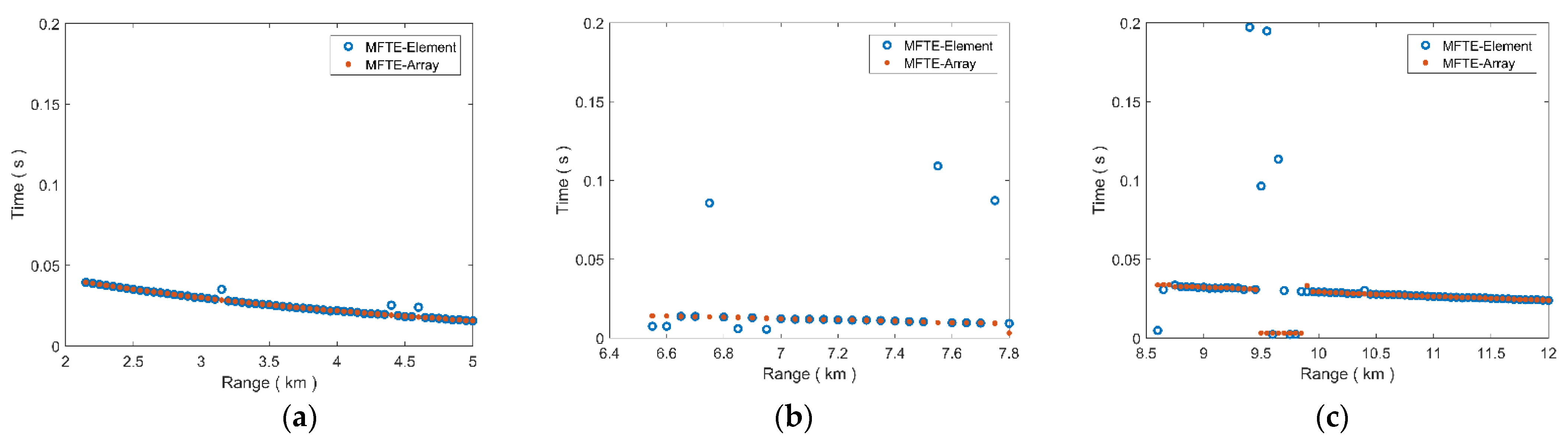
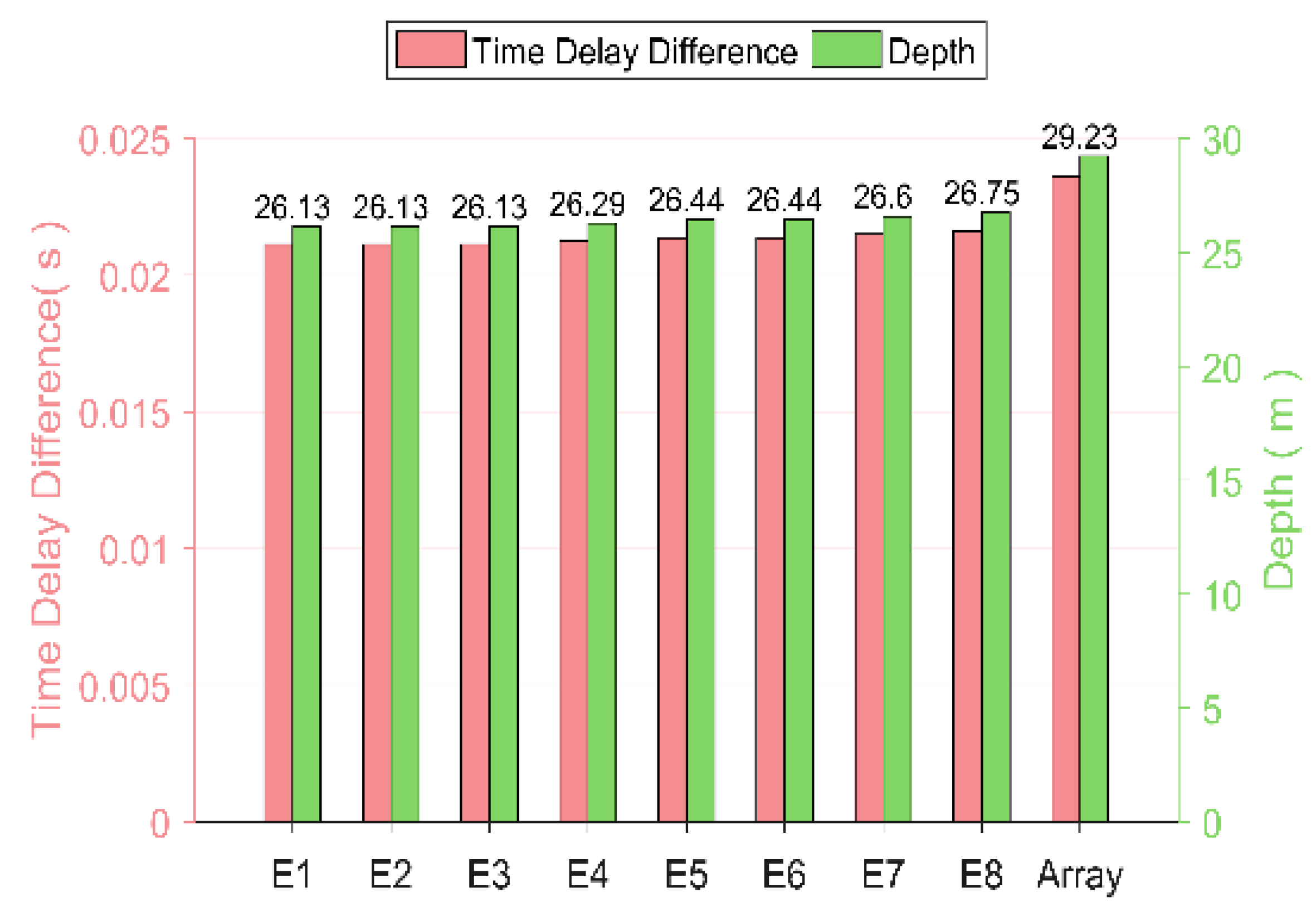
4.3. Performance Analysis

According to the analysis above, the main influencing factors on the depth estimation accuracy include the receiving depth error and the time delay difference error.

The receiving depth used in the simulation and experiments is the depth of the array center. The depths of the first and last elements are used as the receiving depths, respectively, and then the difference in the estimated source depth caused by the difference in the receiving depth of 75 m is only 0.52 m. Therefore, the error caused by the receiving depth can be ignored.

The time delay difference is related to the accuracy of estimated angles. When the angles with maximum energy obtained by beamforming are quite different from the arrival angle of the dominant interference components, the time delay difference extracted from the two peaks of the compensated signal is not accurate. Therefore, this method requires the accuracy of elevation angle estimation.

This method has two limitations, one is that the detectable target depth is constrained by the target bandwidth and the elevation angle. These three parameters satisfy the expression $△F\ge c/\left|z_s\cos \phi \right|$. For the experiment, the maximum elevation angle is 107° and the corresponding maximum bandwidth is 168 Hz. The signal bandwidth used in the sea trial is 150 Hz, which is slightly smaller than the maximum detectable frequency band. The estimated sound source depth at an arrival angle of 107° is less than 30 m (24.2 m). Therefore, the receiving hydrophones should be placed as deep as possible to reduce dependence on the frequency range and improve the accuracy of shallow sound source depth estimation. The other limitation is that this method is only applicable to the deep sea.

5. Conclusions

This paper proposes a method for estimating the depth of an underwater broadband target at medium and short ranges in the deep-sea environment. Both simulation and experimental results confirm the effectiveness of this method in reducing depth errors and avoiding the misjudgment of surface or submerged targets. By using matched filtering technology, the SNR of the received signal is improved and the multipath structure reaching the array is separated. Combined beamforming is applied to the vector hydrophone vertical array to obtain accurate elevation angles. Subsequently, beam processing is used again to enhance the SNR of the received signal, making it suitable for low-SNR environments. The time delay difference is extracted from the compensated beam output, and the target source depth is estimated based on the multipath arrival structure. However, this paper only considers the interference of two contributing eigen-rays, providing a limited degree of correction for the target depth. In the future, we will consider the contribution of multiple eigen-rays to further improve the accuracy of depth estimation.

References

1. Baggeroer, A.B.; Kuperman, W.A. Matched field processing: Source localization in correlated noise as an optimum parameter estimation problem. J. Acoust. Soc. Am. 1988, 83, 571–587. [Google Scholar] [CrossRef]
2. Baggeroer, B.; Kuperman, W.A.; Mikhalevsky, P.N. An overview of matched field methods in ocean acoustics. IEEE J. Ocean. Eng. 1993, 18, 401–424. [Google Scholar]
3. Tollefsen, D.; Dosso, S.E. Matched-field source localization with multiple small-aperture arrays. J. Acoust. Soc. Am. 2015, 138, 1754. [Google Scholar] [CrossRef]
4. Tollefsen, D.; Dosso, S.E. Source localization with multiple hydrophone arrays via matched-field processing. IEEE J. Ocean. Eng. 2016, 42, 654–662. [Google Scholar] [CrossRef]
5. Cao, R.; Yang, K.D.; Ma, Y.L.; Yang, Q.L.; Yang, S. Passive broadband source localization based on a Riemannian distance with a short vertical array in the deep ocean. J. Acoust. Soc. Am. 2019, 145, 567–573. [Google Scholar] [CrossRef]
6. Zhu, F.W.; Zheng, G.Y.; Liu, F.C. Matched arrival pattern-based method for estimating source depth in deep sea bottom bounce areas. J. Harbin Eng. Univ. 2021, 42, 1510–1517. [Google Scholar]
7. Lopatka, M.; Grégoire, L.T.; Nicolas, B.; Cristol, X.; Jérôme, I.M.; Fattaccioli, D. Underwater broadband source localization based on modal filtering and features extraction. EURASIP J. Adv. Signal Process. 2010, 2010, 304103. [Google Scholar] [CrossRef]
8. Conan, E.; Bonnel, J.; Chonavel, T.; Nicolas, B. Source depth discrimination with a vertical line array. J. Acoust. Soc. Am. 2016, 140, 434–440. [Google Scholar] [CrossRef]
9. Xu, G.J.; Zhang, W.H.; Zhu, M.; Guo, J.Z.; Wu, Y.Q.; Zhu, J.H. Research on Underwater Acoustic Target Depth Classification Based on Modal Filtering Characteristics of Long Horizontal Line Array. Int. J. Acoust. Vib. 2022, 27, 3–9. [Google Scholar] [CrossRef]
10. Duan, R.; Yang, K.D.; Ma, Y.L.; Yang, Q.L.; Li, H. Moving source localization with a single hydrophone using multipath time delays in the deep ocean. J. Acoust. Soc. Am. 2014, 136, 159–165. [Google Scholar] [CrossRef]
11. An, L.; Chen, L.J. Underwater acoustic passive localization base on multipath arrival structure. In Proceedings of the 43rd International Congress on Noise Control Engineering, Melbourne, Australia, 16–19 November 2014. [Google Scholar]
12. Yang, K.D.; Yang, Q.L.; Guo, X.L.; Cao, R. A simple method for source depth estimation with multi-path time delay in deep ocean. Chin. Phys. Lett. 2016, 33, 124302. [Google Scholar] [CrossRef]
13. Urick, R.J. Priciples of Underwater Sound, 3rd ed.; MaGraw-Hill: New York, NY, USA, 1983. [Google Scholar]
14. McCargar, R.; Zurk, L.M. Depth-based signal separation with vertical line arrays in the deep ocean. J. Acoust. Soc. Am. 2013, 13, 320–325. [Google Scholar] [CrossRef] [PubMed]
15. Kniffin, G.P.; Boyle, J.K.; Zurk, L.M.; Siderius, M. Performance metrics for depth-based signal separation using deep vertical line arrays. J. Acoust. Soc. Am. 2016, 139, 418–425. [Google Scholar] [CrossRef] [PubMed]
16. Yang, K.D.; Xu, L.Y.; Yang, Q.L.; Duan, R. Striation-based source depth estimation with a vertical line array in the deep ocean. J. Acoust. Soc. Am. 2018, 143, 8–12. [Google Scholar] [CrossRef] [PubMed]
17. Yang, K.D.; Li, H.; Duan, R.; Yang, Q.L. Analysis on the characteristic of cross-correlated field and its potential application on source localization in deep water. J. Comput. Acoust. 2017, 25, 1750001. [Google Scholar] [CrossRef]
18. Duan, R.; Yang, K.D.; Li, H.; Ma, Y.L. Acoustic-intensity striations below the critical depth: Interpretation and modeling. J. Acoust. Soc. Am. 2017, 142, 245–250. [Google Scholar]
19. Duan, R.; Yang, K.D.; Li, H.; Yang, Q.L.; Wu, F.Y.; Ma, Y.L. A performance study of acoustic interference structure applications on source depth estimation in deep water. J. Acoust. Soc. Am. 2019, 145, 903–916. [Google Scholar] [CrossRef]
20. Li, H.; Yang, K.D.; Duan, R.; Lei, Z. Joint Estimation of Source Range and Depth Using a Bottom-Deployed Vertical Line Array in Deep Water. Sensors 2017, 17, 1315. [Google Scholar] [CrossRef]
21. Reeder, B.D. Clutter depth discrimination using the wavenumber spectrum. J. Acoust. Soc. Am. 2013, 135, 1–7. [Google Scholar] [CrossRef]
22. Qi, Y.B.; Zhou, S.H.; Liang, Y.Q.; Du, S.Y.; Liu, C.P. Passive broadband source depth estimation in the deep ocean using a single vector sensor. J. Acoust. Soc. Am. 2020, 148, 88–92. [Google Scholar] [CrossRef]
23. Li, H.; Wang, T.; Su, L.; Wang, W.B.; Guo, X.Y.; Wang, C.; Ma, L. A multi-step method for passive broadband source localisation using a single vector sensor. IET Radar Sonar Navig. 2022, 16, 1656–1669. [Google Scholar] [CrossRef]
24. Yang, S.G.; Li, Y.; Zhang, K.H.; Liu, J.S. A Signal Processing Algorithm Based on 2D Matched Filtering for SSAR. Math. Probl. Eng. 2017, 12, 4047983. [Google Scholar] [CrossRef]
25. Zhao, Z.; Zhao, A.; Hui, J.; Hou, B.; Sotudeh, R.; Niu, F. A Frequency-Domain Adaptive Matched Filter for Active Sonar Detection. Sensors 2017, 17, 897. [Google Scholar] [CrossRef] [PubMed]
26. Jensen, F.B.; Kuperman, W.A.; Porter, M.B.; Schmidt, H. Computational Ocean Acoustics; Springer: New York, NY, USA, 2011. [Google Scholar]
Figure 1. Flow diagram of MFTE method.
Jmse 11 02059 g001
Figure 2. Schematic diagram of a vector hydrophone vertical array.
Jmse 11 02059 g002
Figure 3. Sound speed profile in the deep ocean.
Jmse 11 02059 g003
Figure 4. Schematic diagram of the sound source and array positions in the simulation.
Jmse 11 02059 g004
Figure 5. Received signal by 8th hydrophone before and after MF at (a) 3.5 km; (b) 7 km; (c) 11.5 km.
Jmse 11 02059 g005
Figure 6. Beamforming output within (a) 2.1–5 km; (b) 6.5–7.8 km; (c) 8.6–12 km.
Jmse 11 02059 g006
Figure 7. Arrival structure of eigen-rays for 8th hydrophone within (a) 2.1–5 km; (b) 6.5–7.8 km; (c) 8.6–12 km.
Jmse 11 02059 g007
Figure 8. Received signal for 8th hydrophone and the signal after compensation at (a) 3.5 km; (b) 7 km; (c) 11.5 km.
Jmse 11 02059 g008
Figure 9. Time delay differences extracted from different methods within (a) 2.1–5 km; (b) 6.5–7.8 km; (c) 8.6–12 km.
Jmse 11 02059 g009
Figure 10. Depth estimation results from different methods within (a) 2.1–5 km; (b) 6.5–7.8 km; (c) 8.6–12 km.
Jmse 11 02059 g010
Figure 11. Experimental diagram.
Jmse 11 02059 g011
Figure 12. Received signal of (a) P and (b) Z axes before and after MF by 3rd hydrophone at 2.4 km.
Jmse 11 02059 g012
Figure 13. (a) Beamforming results of four processing methods; (b) Compensated pressure signal at 2.4 km.
Jmse 11 02059 g013
Figure 14. Estimated time delay differences and source depths from data at 2.4 km.
Jmse 11 02059 g014
Figure 15. Received signal of (a) P and (b) Z axes before and after MF by 3rd hydrophone at 7.1 km.
Jmse 11 02059 g015
Figure 16. (a) Beamforming results of four processing methods; (b) Product factor for 74° at 7.1 km.
Jmse 11 02059 g016
Figure 17. Compensated signal for angles of (a) 74°; (b) 107° at 7.1 km.
Jmse 11 02059 g017
Figure 18. Estimated time delay differences and source depths from data at 7.1 km.
Jmse 11 02059 g018