Morphological Modelling to Investigate the Role of External Sediment Sources and Wind and Wave-Induced Flow on Sand Bank Sustainability: An Arklow Bank Case Study

Abstract

Offshore anthropogenic activities such as the installation of Offshore Renewable Energy (ORE) developments and sediment extraction for marine aggregates have been shown to disrupt current flow, wave propagation, and sediment transport pathways, leading to potential environmental instability. Due to the complexity of the interconnected sediment transport pathways in the south-western Irish Sea combined with an increase in planned anthropogenic activities, the assessment of this risk is imperative for the development of a robust marine spatial plan. Subsequently, this study uses two-dimensional morphological modelling to build upon previous studies to assess the dependency of Arklow Bank’s local sediment transport regime on external sediment sources. Additionally, scenario modelling is used to identify vulnerable areas of this offshore linear sand bank to wind and wave-forcing and to examine the nature of this impact. A sediment budget is estimated for Arklow Bank, whereby seven source and nine sink pathways are identified. New evidence to support the exchange of sediment between offshore sand banks and offshore independent sand wave fields is also provided. The areas of the bank most vulnerable to changes in external sediment sources and the addition of wind- and wave-induced flow are analogous. These high vulnerability zones (HVZs) align with regions of residual cross-flow under pure current conditions. The restriction of sediment sources off the southern extent of Arklow Bank impacts erosion and accretion patterns in the mid- and northern sections of the bank after just one lunar month of simulation. Where tidal current is the primary driver of sand bank morphodynamics, wind- and wave-induced flow is shown to temporarily alter sediment distribution patterns. Wind and wave-induced flow can both accelerate and decelerate the east-west fluctuation of the upper slopes of the bank, yet the nature of this impact is inconsistent due to the misalignment of the directionality of these two forces. The methods and new knowledge derived from this study are directly applicable to tidally-dominated environments outside the Irish Sea.

1. Introduction

Sand banks are important sites for benthic habitats, coastal protection, and marine aggregates and often host offshore renewable energy developments. Arklow Bank, in particular, hosts Ireland’s only offshore wind farm (Arklow Wind Park Phase 1), which is earmarked for further expansion (Arklow Wind Park Phase 2) [1] (Figure 1). Additional offshore wind farm projects, at various stages of planning, are located across the south-western Irish Sea. With the acceleration of the offshore renewable energy industry and future needs for aggregate material, the demand for marine resources is increasing. Many of these offshore anthropogenic activities, such as dredging and the installation of offshore renewable energy (ORE) infrastructure, can affect wave propagation, flow patterns, and sediment circulation [2,3,4,5,6,7,8,9]. In the near field, these changes have the potential to alter marine biogeochemistry, including marine life behaviour, phytoplankton dynamics, and benthic habitats [10,11]. In the far field, subsequent physical impacts to the marine environment could be detrimental, causing shoreline change [8,10] or could be beneficial, aiding coastal protection [12,13]. The nature of this impact depends on the local oceanographic regime, the type and size of the ORE development and ORE lay-out configurations, or the volume, scale, and nature of dredged material. This study investigates the physical controls on the sediment transport regime encompassing Arklow Bank, an offshore linear sand bank in the south-western Irish Sea, in order to reduce the risk of environmental instability due to ongoing and planned anthropogenic activities. In order to reduce the risk of negative environmental repercussions following increased offshore anthropogenic activities, a comprehensive understanding of baseline dynamics is imperative to inform environmental risk assessments (EIA) and long-term marine spatial planning.

The south Irish Sea is a tidally-dominated shallow shelf sea environment that exhibits a highly complex hydrodynamic and morphodynamic regime influenced by a tidal symmetry zone and bed load parting zone extending approximately from Ardanary on the Irish coastline to Anglesey on the United Kingdom’s coastline [14] (Figure 1). Additionally, the presence of a tidal node oscillation zone extending from the coastline at Courtown for approximately 39 km provides additional complexity to the hydrodynamics of the region [14] (Figure 1).

Arklow Bank itself displays flood and ebb tidal dominance on the west and east sides of the bank, respectively. This ultimately generates a clockwise residual transport pathway that encompasses the entire bank, facilitating sediment distribution within the morphological cell. This is reflected in bed load transport, whereby sand waves with a mean height and wave length of 3 m and 140 m, respectively, migrate southwards at a mean rate of 23 m/year on the south-eastern side of the bank. Contrastingly, sand waves on the south-western side of the bank display a mean height and wave length of 2.3 m and 123.5 m, respectively, and migrate northwards at a rate of 32.7 m/year [15] (Figure 1). Within this sediment transport cell, Arklow Bank displays a highly mobile upper surficial sediment layer [16,17]. Eight unique hydrodynamic and morphodynamic sub-cells of the bank are identified that display various levels of upper slope east-west fluctuation [17] yet overall long-term bank base stability is maintained. This highly mobile upper layer has posed issues for anthropogenic activities, whereby wind turbines installed during Arklow Wind Park Phase 1 have been affected by scour development [18].

Figure 1. (a) Overview of Irish Sea oceanographic phenomena impacting this study site (b) the area of interest, Arklow Bank. Panel (a) bathymetry source: EMODnet [19] where MSL is mean sea level; Panel (b) bathymetry source: INFOMAR (https://www.infomar.ie/, accessed on 20 March 2020) where LAT is the lowest astronomical tide. Adapted from Creane et al. [17].

Figure 1. (a) Overview of Irish Sea oceanographic phenomena impacting this study site (b) the area of interest, Arklow Bank. Panel (a) bathymetry source: EMODnet [19] where MSL is mean sea level; Panel (b) bathymetry source: INFOMAR (https://www.infomar.ie/, accessed on 20 March 2020) where LAT is the lowest astronomical tide. Adapted from Creane et al. [17].

Evidence of a semi-open circulatory residual sediment transport regime over Arklow Bank is presented by Creane et al. [15], who identify multiple residual transport pathways that facilitate the recycling of sediment material between offshore sand banks and offshore independent sand deposits. In this way, sediment passes in and out of Arklow Bank’s local sediment transport cell, implying an influence of external sediment sources on Arklow Bank’s sustainability and longevity. Furthermore, Creane et al. [17] use a coupled two-dimensional hydrodynamic and sediment transport model to investigate the hydrodynamic processes that drive upper bank mobility while maintaining long-term bank base stability. Ultimately, the positioning of multiple anticlockwise residual current eddies along the circumference of this main large clockwise residual current eddy both facilitates and inhibits upper bank mobility and promotes long-term base bank stability. These eddies also promote sediment exchange along the bank margin. Furthermore, a strong hydrodynamic-morphodynamic feedback loop is evident along the length of the upper slopes of the bank. Both on-bank clockwise mobile and stationary residual current eddies, the generation of ‘narrow’ residual cross-flow zones, and the concept of a ‘threshold slope angle’ play a role in controlling maximum horizontal and vertical bed level fluctuation limits [17].

Building upon this pure current-based approach, it is important to have a comprehensive understanding of other physical factors impacting this sediment transport regime, namely wind, waves, and external sediment sources.

In shallow areas of the bank, where the oscillatory motion of waves reaches the sea floor, the combined tidal current- and wave-induced bed shear stress allows grains to exceed the threshold of motion more readily, thus increasing erosion and sediment transport. Coughlan et al. [16] show that Arklow Bank displays a mobilisation frequency index (MFI) of approximately 70% under pure current conditions over a one-year period. Although the dominant seabed disturbance process is tidal currents, areas of the bank display an MFI of up to 20% under pure wave-induced bed shear stress [16]. Sediment stirring caused by this increased erosion is shown to modify the shape of sand bank-associated sand waves and influence sand wave migration rate and direction [15]. Furthermore, wave-induced flow has been shown to influence net sediment transport directions [20,21,22]. Mitchell et al. [22] showed that surface waves enhance sand transport during slack tide by maintaining particles above the threshold of motion and providing a bed shear stress vector in the direction of wave propagation. Additionally, the wind-tidal current interaction is highly complex, whereby in areas of low tidal amplitudes, even moderate wind speeds can reverse residual tidal currents [23,24]. In this way, the most vulnerable areas of Arklow Bank to wind and wave conditions and the nature of their impact are important to comprehend.

To elucidate the impact of external sediment on Arklow Bank’s sediment transport regime and morphodynamic patterns, the coastal engineering concept, the ‘sediment budget’, will be adopted. The development of a sediment budget is a commonly used tool to understand how a coastal system functions [25,26,27]. A sediment budget balances the volumes of sediment entering (sources) and leaving (sinks) a selected coastal region with the resulting erosion or accretion in that cell within a defined period of time. This is summarised in the following equation [27]:

$$Residual=\sum Q_{source}-\sum Q_{sink}-∆V+P-R$$

(1)

whereby the Q-terms represent the sediment entering and leaving the cell, the P- and R-terms represent the sediment that is ‘placed’ or ‘removed’ from the cell by anthropogenic activities such as beach nourishment or dredging, respectively, and $∆V$ is the volume change in the cell. The resulting “residual” is an indicator of how balanced the cell is and should be zero if all parameters are accounted for. The most common approach to developing a sediment budget is to use the most known variables, such as volume change data and placement and removal data, as the foundation of the budget. Subsequently, a range of longshore transport rates and other relative magnitudes are applied to solve for the budget. This study will test the applicability of this coastal engineering concept in an offshore setting to estimate a sediment budget for Arklow Bank. Once estimated, the impact of external sediments on the sediment transport regime and morphodynamics can be assessed.

When developing robust hydrodynamic and morphological models for offshore environments, the utilisation of the most efficient mesh resolution after considering specific study aims and objectives, site-specific environmental considerations, computational power and run time, and project budget and timeline is imperative to achieving the best results. Depending on these variables, various mesh types (unstructured or structured) [28] and resolution have been utilised to model regional scale hydrodynamic and sediment transport trends [14,16,29], and specific bedform dynamics such as sand waves under both two-dimensional (2D) [30], two-dimensional vertical (2DV) [31], and three-dimensional (3D) modelling techniques [32,33], and sand banks [20,34,35,36,37,38]. Performing a mesh sensitivity analysis is a useful technique in the decision-making process.

Specifically, this study addressed the following hypothesis:

‘Morphodynamics of offshore sand banks in tidally-dominated continental shelf seas are dominated by tidal current processes yet are influenced by other phenomena, including external sediment sources and wind and wave processes.’ Based on this hypothesis, this study aimed to:

• Conduct a numerical model mesh sensitivity analysis to define the most efficient spatial resolution that facilitates the investigation of various processes controlling Arklow Bank morphodynamics;
• Estimate a sediment budget for Arklow Bank;
• Examine the influence of external sediment sources on the local sediment transport regime and bank morphodynamics;
• Identify the most vulnerable areas of the bank due to wind and wave-induced flow and the nature of this impact.

2. Materials and Methods

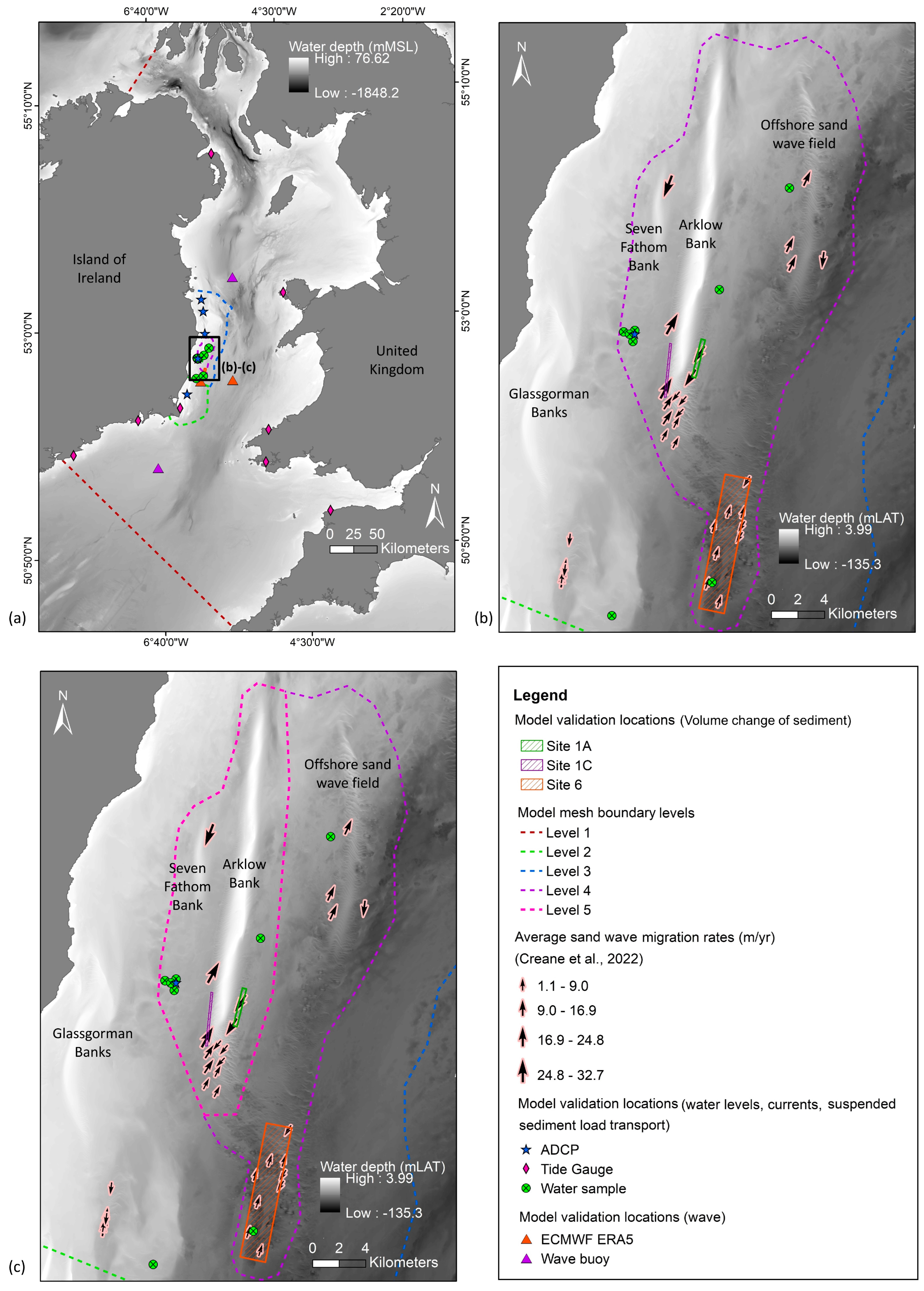
2.1. Numerical Model Set-Up and Validation

2.1.1. Hydrodynamic and Sediment Transport Model

A dynamically coupled two-dimensional (2D) hydrodynamic and sediment transport model was developed using the MIKE 21 suite of tools [39,40,41], the extent of which is outlined in Figure 2. The model utilises an unstructured flexible mesh, which facilitates a varied spatial resolution across the model domain (Figure 2). A variation of four to five levels of refined mesh resolution is utilised in this study, details of which are provided in Section 2.2. For hydrodynamic model validation, water levels were assessed using data from eight tide gauges and four Acoustic Doppler Current Profiler (ADCP) datasets located within the model domain (Figure 2). A strong positive correlation was evident between all measured and simulated water levels, where the average correlation coefficient across all locations was 0.99. Similarly, current speeds and directions were assessed at four ADCP locations, where a strong positive correlation was evident, ranging from 0.84 to 0.95. The full setup and validation details of the hydrodynamic model are provided in Creane et al. [17,42].

The MIKE 21 hydrodynamic and sand transport modules were dynamically coupled to allow morphological development to be captured. This was carried out by updating the bathymetry for every timestep with net sedimentation. The pure-current sediment transport theory used in this model was the Engelund and Hansen [43] total-load transport theory. A varying grain diameter ($D_{50}$) map was defined for the model domain comprising both surficial and synthetic sediment samples (Figure 3). In the area of interest, these samples were predominantly based on in-situ surficial sediment samples. Where data was limited, the synthetic ‘sand $D_{50}$’ dataset developed by Wilson et al. [44] was utilised, alongside a second synthetic dataset that was generated by cross-correlating in-situ sediments with backscatter and the EMODnet seabed substrate map. The sediment transport model was validated in multiple locations within the area of interest utilising a variety of in-situ datasets, including water sample-derived suspended solids concentration (SSC), ADCP-derived SSC, and high-resolution repeat bathymetry datasets (Figure 2). The full set-up and validation details of the sediment transport model are provided in Creane et al. [17,42].

2.1.2. Spectral Wave Model

A validated MIKE 21 spectral wave model [45] was developed using the same domain as the hydrodynamic model outlined in Section 2.1.1 (Figure 2). This fully spectral formulation is based on the wave action conservation equation as described in Komen et al. [46] and Young [47], where the directional-frequency wave action spectrum is the dependent variable. The discretization in the geographical and spectral spaces is performed using a cell-centered finite volume method [45]. The model can include wave growth by the action of wind, non-linear wave-wave interaction, wave-current interaction, refraction and shoaling due to depth variations, the effect of time-varying water depth and flooding and drying, and dissipation due to white capping, bottom friction, and depth-induced wave breaking. This fully spectral model can simulate both swell and wind-generated waves. The quadruplet-wave interaction is described by the Discrete Interaction Approximate (DIA) [46]. White capping-driven energy dissipation is based on the formulation of Hasselmann [48] and Bidlot et al. [49], where the final dissipation coefficients used in the model, $C_{dis}$ (Cdis) and $\delta$ (DELTAdis), are 3.5 and 0.5, respectively. As waves propagate into shallow water, the orbital wave velocities penetrate the water depth, and the source function due to wave-bottom interaction becomes important. Dissipation due to bottom friction depends on the hydrodynamic and sediment conditions, as described in Johnson and Kofoed-Hansen [50]. To account for bottom friction, a Nikuradse roughness value [51] of 0.04 m was applied as recommended by Weber [52]. Depth-induced wave breaking is calculated based on empirical formulations by Battjes and Janssen [53]. In this case, the Gamma parameter used in the breaking formulation was constant at 0.8. The effect of wind forcing on the surface stress is incorporated into the model using empirical relationships that include density, drag coefficient, and wind speed.

A wind field comprising wind speed and direction at 10 m above sea level has been incorporated into the model using the European Centre for Medium-Range Weather Forecasts’ (ECMWF) ERA5 Climate Reanalysis dataset. This wind field varies in time (1 h intervals) and over the entire domain at a spatial resolution of 0.25° × 0.25°. The two open boundaries (Figure 2) are forced with hourly significant wave height, peak wave period, mean wave direction, and directional standard deviation extracted from the European Centre for Medium-Range Weather Forecasts’ ERA5 Climate Reanalysis dataset at 0.5° × 0.5° resolution. The Global Tide Model developed by DTU Space [54] provides one-hour water levels covering the whole model domain. This ensures that the changes in wave conditions due to varying water depths resulting from tides are properly modelled. The wave model outputs include significant wave height ($H_s$), peak wave period ($T_p$), mean spectral wave zero-upcrossing period ($T_{02}$), mean wave direction ($MWD$) and three components of radiation stresses ($S_{xx}, S_{yy}, S_{xy}$) which were output at 1 h intervals for model calibration and validation. Calibration was carried out by altering bottom friction, white capping, and wave breaking parameters.

Data from the M2 (53.480° N, 5.425° W) and M5 (51.690° N, 6.704° W) wave buoys were downloaded from the Met Éireann online delivery system for a period between 2014 and 2016 for calibration and validation purposes. In order to compare the MIKE 21 simulated spectral zero crossing period ($T_{02}$) to the significant wave period ($T_s$) recorded by the wave buoys, the measured dataset ($T_s$) was converted to $T_{02}$ using the following equation [55]:

$$T_s=1.14T_{02}$$

(2)

Due to the limited amount of in-situ data available across the model domain, an additional validation was carried out using two data points extracted from the ECMWF ERA5 climate reanalysis model to ensure a more robust validation. The location of these two additional validation points is provided in Figure 2 and

Table 1. Comparison between the model and measured M2 and M5 datasets and the model and output from the ERA5-ECMWF dataset at locations shown in Figure 2. The indices shown are bias, the root-mean-square error (RMSE), the correlation coefficient (R), and the scatter index (SI).

Dataset	Dataset Type	Location	Significant Wave Height (m)
			Bias (m)	RMSE (m)	R	SI (%)
M2	Measured (wave buoy)	53.480° N, 5.425° W	−0.03	0.24	0.98	19.20
M5	Measured (wave buoy)	51.690° N, 6.704° W	−0.19	0.35	0.97	16.84
ERA5-ECMWF 1	Climate reanalysis (modelled)	52.5° N, 6° W	0.06	0.20	0.98	16.80
ERA5-ECMWF 2	Climate reanalysis (modelled)	52.5° N, 5.5° W	−0.04	0.23	0.98	13.37

.

The level of agreement between the model output and these observed/ERA5 datasets are assessed both visually and statistically. Visual comparisons allow the assessment of the shape, trend, range, and limits of the model and observed/ERA5 datasets (Figure 4), whereas statistical comparisons determine the degree to which the model fits the observations within defined calibration limits. A number of statistics were generated to assess the fit between measured/ERA5 and simulated datasets (Table 1 and Figure 4). Where the correlation coefficient is a measure of linear correlation between measured and simulated variables, bias represents the mean difference between both datasets. The root-mean-square-error (RMSE) is the standard deviation of residuals, and the scatter index presents the percentage of the RMS difference with respect to the mean observation. The comparisons between in-situ measurements and simulated predictions for $H_s$, $T_{02}$ and $MWD$ generally showed a good fit; time series plots are presented in Figure 4. A strong positive relationship is evident between the measured or ERA5 dataset and the simulated timeseries, with an average R value of 0.98 across all four data points (Table 1; Figure 4g–j). Additionally, a scatter index of <20% is evident across all sites, revealing a good correlation.

2.2. Scenario Modelling

Five scenario model runs were constructed to address the hypothesis outlined in Section 1. These are summarised in

Table 2. Overview of scenario modelling.

Model Runs	Aim of Model Run	Description	Mesh Levels
Run 1	To simulate baseline conditions using a higher spatial resolution over Arklow Bank	Hydrodynamic module: - Pure current Sand transport module: - Baseline conditions	Five
Run 2	To simulate baseline conditions using a lower spatial resolution over Arklow Bank	Hydrodynamic module: - Pure current Sand transport module: - Baseline conditions	Four
Run 3	To test the influence of external sediment sources on baseline conditions (Run 2)	Hydrodynamic module: - Pure current Sand transport module: - Designated ‘immobile’ zones in identified sediment source areas.	Four
Run 4	To test the influence of wind on baseline conditions (Run 2)	Hydrodynamic module: - Current - Inclusion of wind and surface pressure grid series (1 h temporal resolution; 0.25° spatial resolution) Sand transport module: - Baseline conditions	Four
Run 5	To test the influence of combined wind and wave on baseline conditions (Run 2)	Hydrodynamic module: - Current - Inclusion of wind and surface pressure grid series (1 h temporal resolution; 0.25° spatial resolution) - Inclusion of wave radiation stresses produced from separate spectral wave models. Sand transport module: - Baseline conditions	Four

. Run 1 was previously executed by Creane et al. [17] and produces one-year baseline sediment transport conditions over Arklow Bank under pure current conditions, utilising a relatively high-resolution mesh. The unstructured flexible mesh contains five levels of refinement, the highest of which is 50 m to 80 m over Arklow Bank and Seven Fathom Bank, in order to resolve the main features of the bank at an adequate scale to address the objectives of Creane et al. [17] (Figure 2;

Table 3. Resolution details of the unstructured flexible triangular mesh used in scenario modelling. Adapted from Creane et al. [17].

Mesh Levels		Description	Mesh Utilised
			Original Study	Current Study
5 levels	Level 5	50 to 80 m over Arklow Bank and Seven Fathom Bank	Creane et al. [17]	Run 1
	Level 4	150 to 200 m encompassing the Arklow Bank system, including offshore independent sand wave fields identified in Creane et al. [15]
	Level 3	500 m to 600 m buffer zone, extending from the approximate −70 m water depth contour to the coastline from Howth Head (53.37861°, −6.057222°) to Courtown (52.645°, −6.228333°), and covering any sand banks outside these areas off the south-east coast of Ireland
	Level 2	800 m to 1000 m, extending along the −70 m contour to the coast from Courtown to Carnsore Point (52.17056°, −6.355278°)
	Level 1	2500 m to 3000 m resolution for the rest of the model domain
4 levels	Level 4	150 m to 200 m around the Arklow Bank system (approximately 7.2 km2)	Creane et al. [42]	Run 2, 3, 4, 5
	Level 3	Same as Level 3 above.
	Level 2	Same as Level 2 above.
	Level 1	Same as Level 2 above.

).

Run 2 to Run 5 are new simulations carried out specifically for this body of work (Table 3). Run 2 represents one-year baseline sediment transport conditions over Arklow Bank under pure current conditions, utilising a relatively lower resolution mesh over Arklow Bank. This unstructured mesh contains four levels of refinement, with the highest spatial resolution being 150 to 200 m, encompassing the Arklow Bank system [42] (Figure 2; Table 3). A mesh sensitivity study was carried out by comparing outputs from Run 2 to Run 1 to ensure adequate quality and applicability of this four-level mesh in addressing this study aims.

Run 3 was used to assess the influence of external sediment sources on Arklow Bank’s local sediment transport regime. Firstly, the hydrodynamic and sediment transport model outputs from Run 2 were used to estimate a sediment budget for Arklow Bank. On completion, two significant sediment source areas were identified and designated as ‘immobile’ zones in the sediment transport model of Run 3. This was executed by adjusting the median grain size ($D_{50}$) of these ‘immobile zones’ to 1 m to ensure the threshold of motion is not exceeded by bed shear stress exerted on the seabed. The outputs from Run 3 were compared against baseline outputs from Run 2 to assess the response of the sediment transport regime to this change. More details are outlined in Section 3.3.

Run 4 utilised the model set-up of Run 2 as a foundation but included an additional 2D spatially-varying grid series of u- and v-wind velocity components and surface pressure in the hydrodynamic model. This hourly dataset has a 0.25 ° spatial resolution and was sourced from the European Centre for Medium-Range Weather Forecasts (ECMWF) ERA5 dataset. Run 4 assessed the influence of wind on Arklow Bank’s sediment transport regime.

Run 5 built upon Run 4 to assess the influence of wave-induced flow on this sediment transport system. Firstly, the spectral wave model described in Section 2.1 was run for a one-year simulation period in order to generate radiation stresses for the entire model domain at a 1 h temporal resolution. Radiation stresses are second-order stresses due to the breaking of short-period waves. They acted as driving forces for the mean flow and can be used to calculate wave-induced flow. The three components of radiation stresses ($S_{xx}, S_{yy}, S_{xy}$) were thus included in the hydrodynamic simulation of Run 5.

3. Results and Discussion

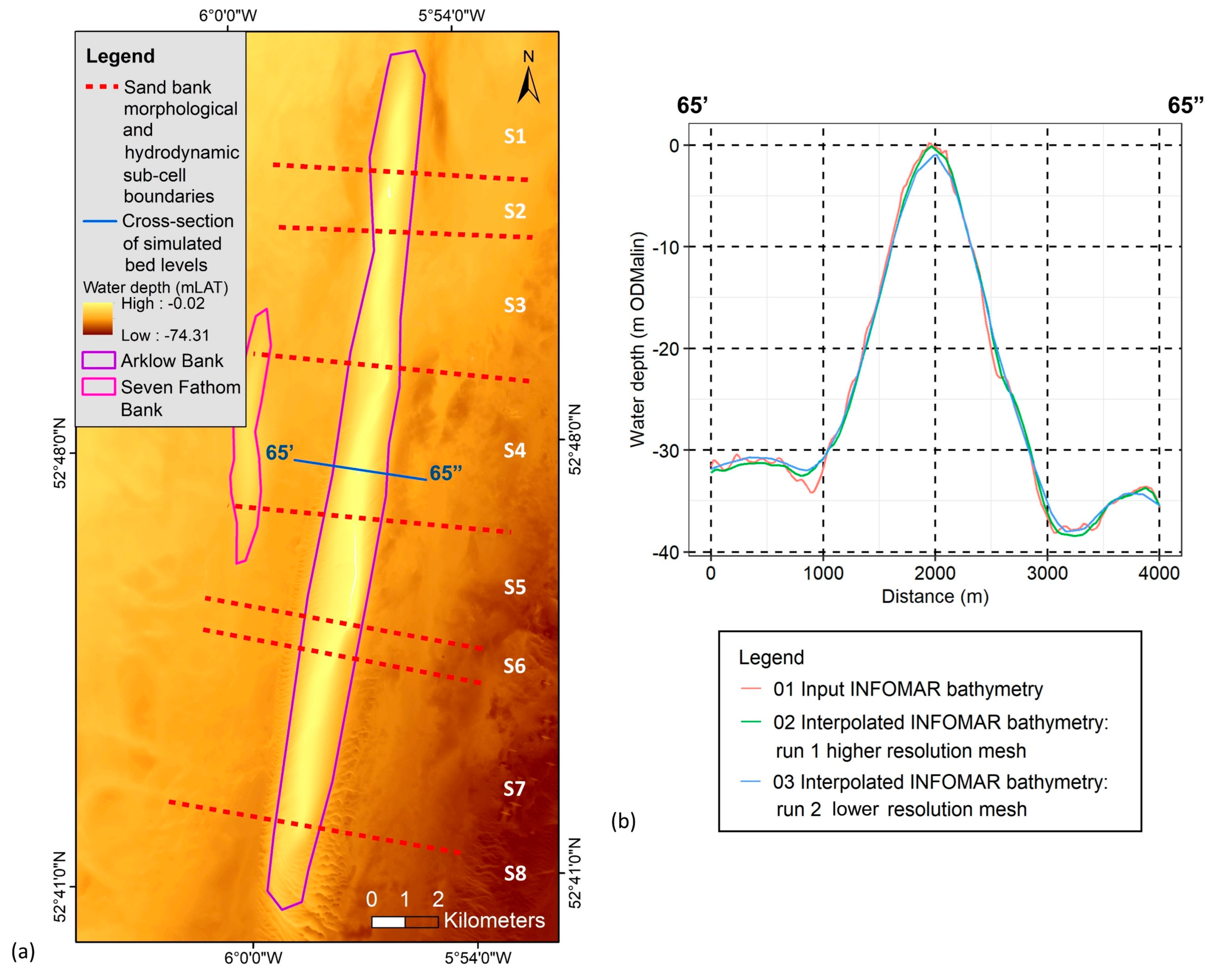
3.1. Mesh Sensitivity Analysis

The hydrodynamic and morphodynamic trends of Run 1 are described in detail in Creane et al. [17], which are summarised in Figure 5. As outlined previously, a large clockwise residual current eddy encompasses the bank, ultimately circulating sediment throughout the morphological cell. A number of anticlockwise residual tidal current eddies are positioned along the circumference of this residual eddy, both facilitating and inhibiting east-west upper slope fluctuation and controlling long-term bank base stability. These also facilitate sediment transfer in and out of the bank’s local sediment transport system. The bank base is described as being relatively stable over time, but the upper slopes are highly dynamic, fluctuating on an approximate east-west axis [17]. The bank is split into eight hydrodynamically and morphodynamically unique sub-cells, whereby sub-cells 1, 3, 7, and 8 are morphologically mobile zones, sub-cells 2 and 6 are relatively stable, and sub-cell 4 is more complex, displaying intermixed zones of stable and mobile upper slopes. East-west fluctuation of the upper slopes is further controlled by both stationary and mobile on-bank clockwise residual tidal current eddies and the development of transient ‘narrow’ zones of residual cross-flow [17].

When comparing simulated current residuals between the high- and low-resolution model runs (Run 1 and Run 2, respectively), both gridded to 200 m resolution, broad hydrodynamic trends are consistent (Figure 6). For example, the off-bank anticlockwise residual current eddies, Eddy C, D, F, and H; one partial anticlockwise current flow, Eddy G; and the clockwise current eddies over the southern tip of the bank, Eddy I, are all present and located in similar positions in both datasets (Figure 6). These current eddies are most likely responsible for the stable positioning of the bank over time and facilitate the transfer of sediment in and out of the bank’s sediment budget cell [17]. Therefore, on a regional level, the inferred hydrodynamic and sediment transport processes remain unchanged when transitioning from a high-resolution mesh to a lower-resolution mesh. Additionally, Figure 7c represents the difference in bed level at t12mo between Run 1 and Run 2. The lack of bed level change (close to 0 m) on the lower slopes of the bank and along the edge of the sediment budget cell in this figure reiterates the ability of the low-resolution mesh to capture regional processes.

On a local level, Figure 7c shows a 12.1 m to −11.3 m difference in bed level on the upper slopes along the length of the bank. Cross-sectional analysis of bed levels over a one-year period reveals that these changes are a result of differences in the timing of east-west fluctuations at various points along the bank. A failure of the low-resolution mesh to fully capture the details of the hydrodynamic-morphodynamic response system, identified from Run 1 in Creane et al. [17], across the upper slopes and crest of the bank, is highlighted.

Previously identified morphological ‘stability’ zones, namely sub-cells 2, 4, and 6, from Run 1, remain quite stable in Run 2. Representative cross-sections are provided in Figure 8. This is consistent with the relatively lower bed level difference between Runs 1 and 2 (Figure 7c) at these stability sections in comparison to the rest of the bank. However, minor differences between the two runs are noted in these stability areas. These are mainly due to the inability of the lower-resolution input bathymetry to fully capture the detailed shape of the bank (Figure 7b and Figure 9b), whereby natural variances in water depth occur across the bank between the two input meshes (for example, cross-section L65 in Figure 9).

This natural variance in the interpolated bathymetry (Figure 7b and Figure 9b) impacts the previously identified mobile sections of the bank to a higher degree, whereby the low-resolution mesh does not capture the morphological details required to model the hydrodynamic-morphodynamic response system appropriately (Figure 10). In particular, the slope threshold, identified as a potential hydrodynamic response stimulator [17], could not be captured accurately in the low-resolution model simulation. As a result, the difference in the timing of the east-west fluctuation and the vertical and horizontal maximum limits of the upper slopes between the two model results is highest in the high mobility zones. Representative cross-sections of this phenomenon are presented in Figure 10.

Ultimately, the change in mesh resolutions does not influence regional hydrodynamics. Therefore, when considering all project variables, including computational time, project objectives, and site-specific environmental conditions, the low-resolution model is adequate to develop a sediment budget for Arklow Bank in order to test the influence of external sediment sources on the morphological cell. Run 2 is also deemed adequate to identify vulnerable areas of the bank to wind and wave-induced flow and the nature of this influence.

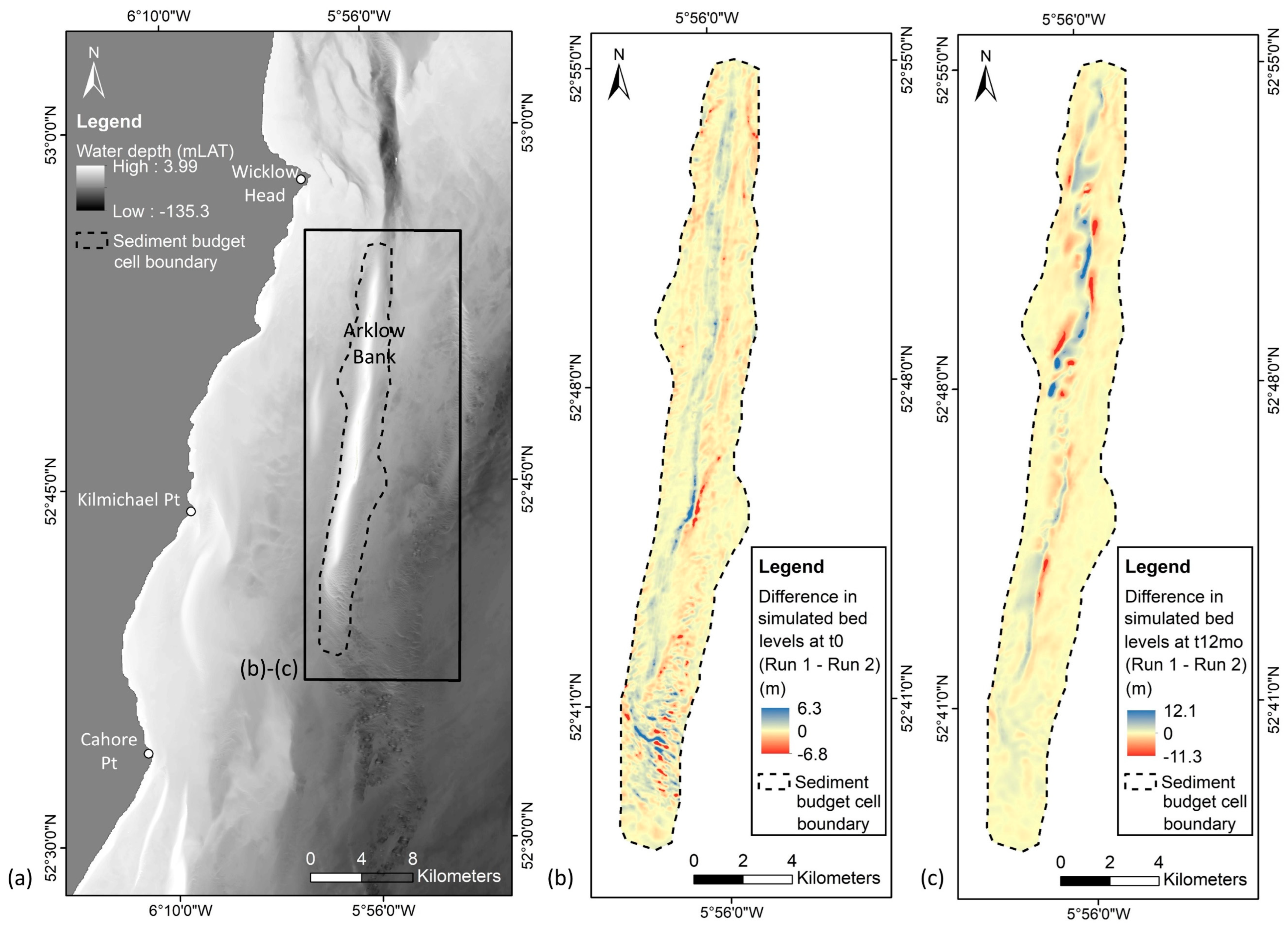
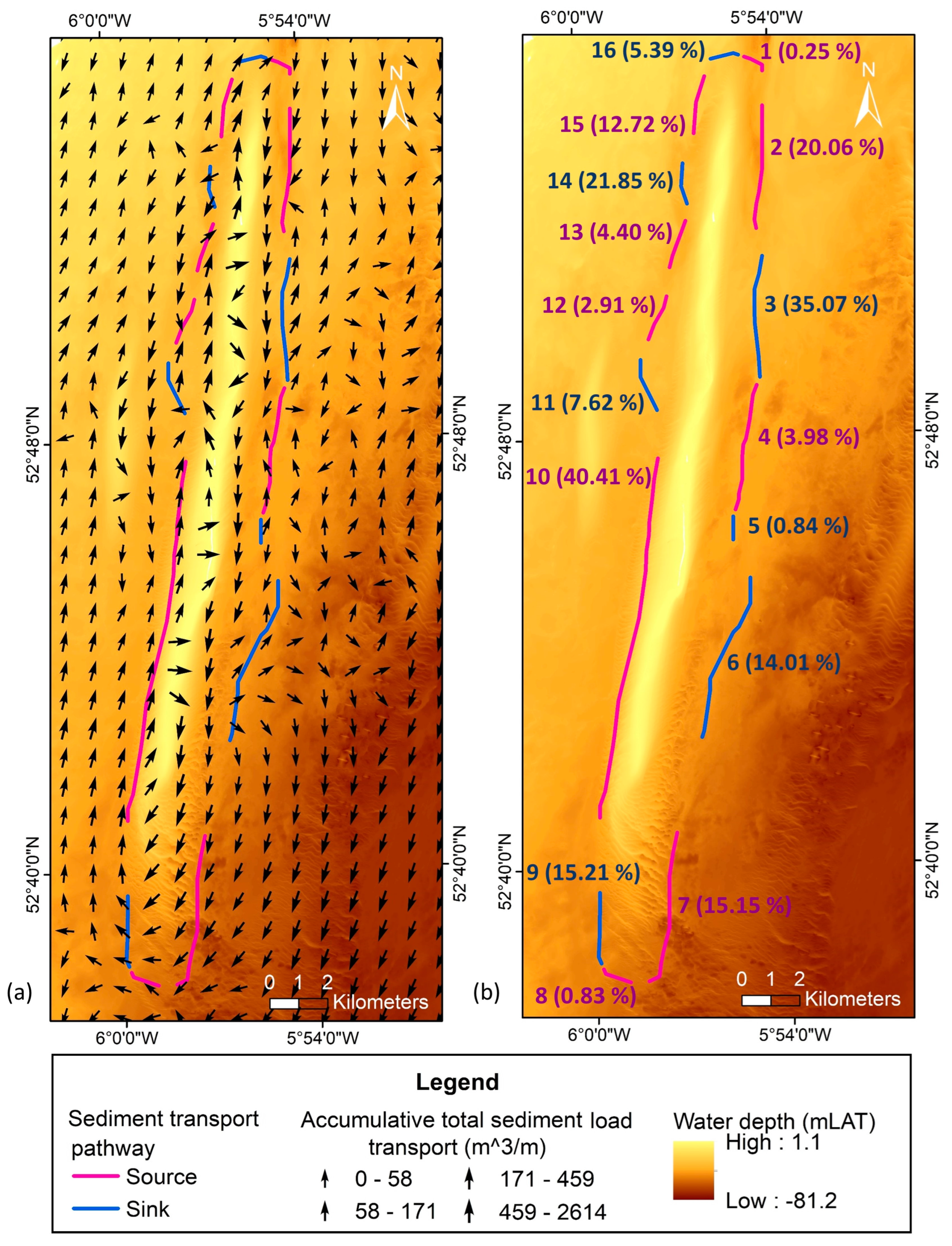
3.2. Sediment Budget

The sediment budget cell boundary and associated source and sink pathways were defined through modelled accumulative total sediment load transport after a one-year simulation period under pure current conditions (Run 2) (Figure 11). The resulting x- and y-velocity components were gridded to a 200 m resolution grid and plotted as magnitude and direction in ArcGIS v10.8. The location of the defined cell boundary was compared, and quality was controlled against the clockwise circulatory flow cell encompassing Arklow Bank and anticlockwise flow cells located on the outside of this main morphological cell, identified through tidal current residuals from the first simulated month (Figure 5). These source and sink pathways were also compared against the structure of the bank, using bathymetry derivatives, e.g., slope, to ensure location accuracy. As expected, the nature of the accumulative total load transport pathway vectors and residual tidal current vectors is quite similar throughout the one-year period (Figure 6b and Figure 11a).

The volume of sediment crossing each defined source and sink cross-section was calculated for a one-year period. At the same time, the simulated volume change over the same time period was calculated. A balanced sediment budget equation was achieved, from which the percentage of the total source or sink sediment volumes was defined for each pathway. These are displayed in Figure 11. Seven sink and nine source pathways were defined. The largest amount of external sediment source enters the morphological cell through cross-sections 2 (20.06%), 7 (15.15%), 10 (40.41%), and 15 (12.72%), whereas the highest volume of sediment leaving the cell passes through pathways 3 (35.07%), 9 (15.21%), and 14 (21.85%).

As discussed by Creane et al. [17], a complex hydrodynamic system drives sediment exchange along the full circumference of the cell boundary. Residual transport vectors, derived from modelled accumulative total sediment transport and tidal current, show that on the eastern side of the bank, sink pathways 3, 5, and 6 facilitate sediment transport out of the local transport system. From here, partial sediment load returns via pathways 2, 4, and 7, while partial load is transported towards an independent offshore sand wave field approximately 8 km east of Arklow Bank (sand wave field 1 in Figure 12) [15]. According to Creane et al. [15], sediment then either (i) returns back to the offshore sand bank, in this case via source transport pathways 7 and 8, or (ii) the offshore independent sand wave field acts as an intermediary stepping stone to independent sand wave fields further offshore (sand wave field 2 in Figure 12). Creane et al. [15] use a combination of environmental variables and theoretical factors to determine the mechanism of sediment transport in this circulatory residual transport pathway. Ultimately, this is predominately controlled by tidal asymmetry. For example, over the ‘transition zone’ where sediment grain sizes are relatively coarser in between the sand bank and the offshore independent sand wave field, residual current magnitudes are high along these transport paths, indicating a strong tidal asymmetry, which correlates with suspended load sediment transport dominance [15].

This study supports this mechanism through the use of sediment transport modelling under pure current conditions. The simulated one-year mean suspended sediment concentration (SSC) is displayed in Figure 12b. As suspected, the results show high SSC over the offshore sand bank and offshore sand wave fields where mobile bedforms and localised sediment transport systems are present. However, Figure 12b also highlights residual ‘plumes’ of SSC over the coarser-grained transition zone, correlating directly with the residual transport pathways derived from residual currents and accumulative total load sediment transport over the same period. The estimation of simulated bed load/suspended load dominance over a one-year period also proves useful in an attempt to support this hypothesis. In the coarse-grained transition zones, suspended load dominance correlates well with the location of these higher residual SSC concentrations, most notably A to D in Figure 12b,c. This provides additional support for the sediment exchange relationship between offshore sand banks and independent sediment wave fields identified by Creane et al. [15].

The external sediment sources at the northern section of the bank can be linked to a sediment transport pathway originating from the on-land headland, Wicklow Head, whereby a south-eastward residual transport pathway is evident, originating from Wicklow Head and entering Arklow Bank’s main morphological cell through source pathway numbers 1 and 2 (Figure 13b) [14]. Additionally, high-resolution modelling of residual tidal currents reveals a residual anticlockwise eddy over the submarine channel, Wicklow Trough [56,57], similar to the trend identified in Creane et al. [14] and Creane et al. [15] (Figure 13b). This potentially acts as a sediment accumulation/deposition zone for eroded sediment from the encompassing shallower Codling Platform [14]. When analysing the one-year accumulative total load sediment transport vectors, a predominant southward sediment transport pathway is evident, streamlined through the Wicklow Trough towards the northern tip of Arklow Bank and partially through source pathways 1 and 2 (Figure 13c). These pathways comprise a combined 20.31% of total external sediment sources. In this way, the Wicklow Trough has the potential to focus sediment transport from the bed load parting zone [14] to Arklow Bank. This is consistent with the work of Coughlan et al. [58], in which areas of active erosion and sediment transport were identified in the Wicklow Trough through the use of geophysical and geological datasets.

However, due to the ‘scoured’ nature of the bed load parting zone (Figure 1) [14], there is a higher potential for currents at the southern half of the bank to carry sediment compared to those focused through this submarine channel. In this way, pathways 7, 8, and 10 comprise 56.39% of the total external sediment sources for the Arklow Bank. From analysing residual currents and total sediment transport load residuals over a one-year period, sediment sources at the southern extent of the bank (i.e., pathways 7, 8, and 10) originate from multiple potential sources, including:

i.

Sink pathways 6 and 9.

ii.

Recycling of sediment from the offshore independent sand wave field (8 km east of Arklow Bank) (sand wave field 1 in Figure 12) [15].

iii.

A pathway flowing north-eastward from the northern tip of the Glassgorman Banks (Figure 13a,d) and Kilmichael Point (on-land headland) (Figure 13a,d) towards pathway 10.

iv.

A pathway identified by Creane et al. [15] originates from the northern extent of Blackwater Bank, flows over an offshore sand wave field approximately 10 km off the south-eastern end of Arklow Bank, and continues north-westward across the southern extent of the bank.

In addition, the western side of the bank contains a dynamic exchange system between Arklow Bank and the Seven Fathom Bank through source and sink pathways 10 to 15, potentially recycling material between one another and promoting long-term stability.

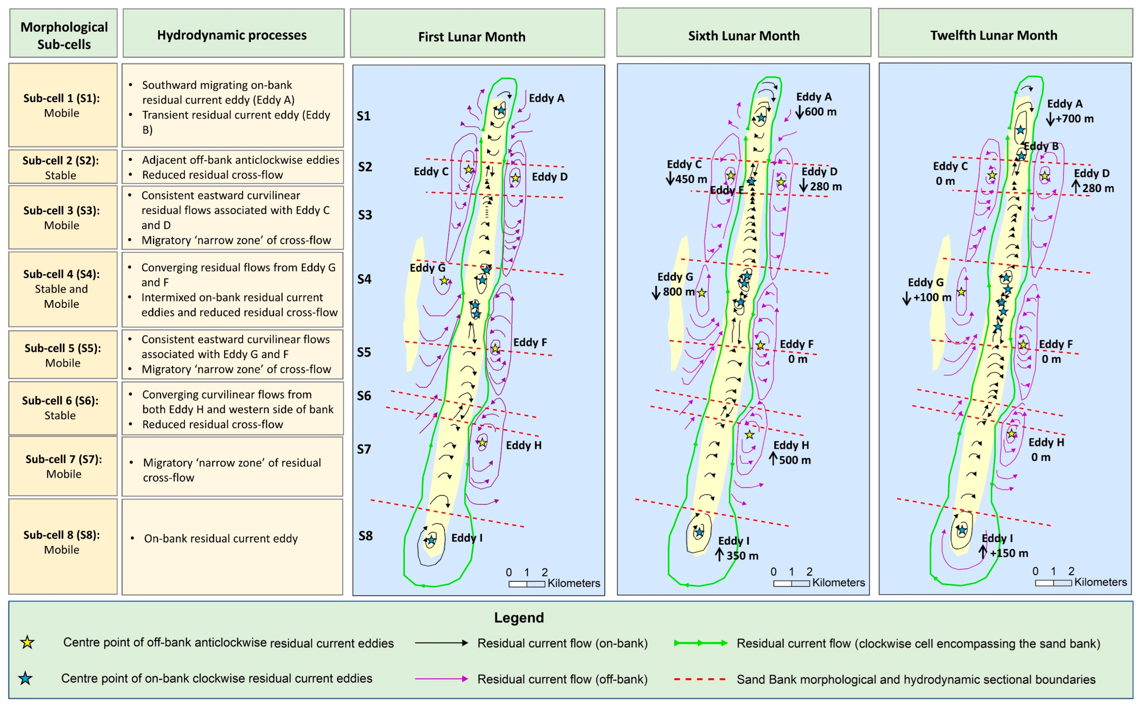
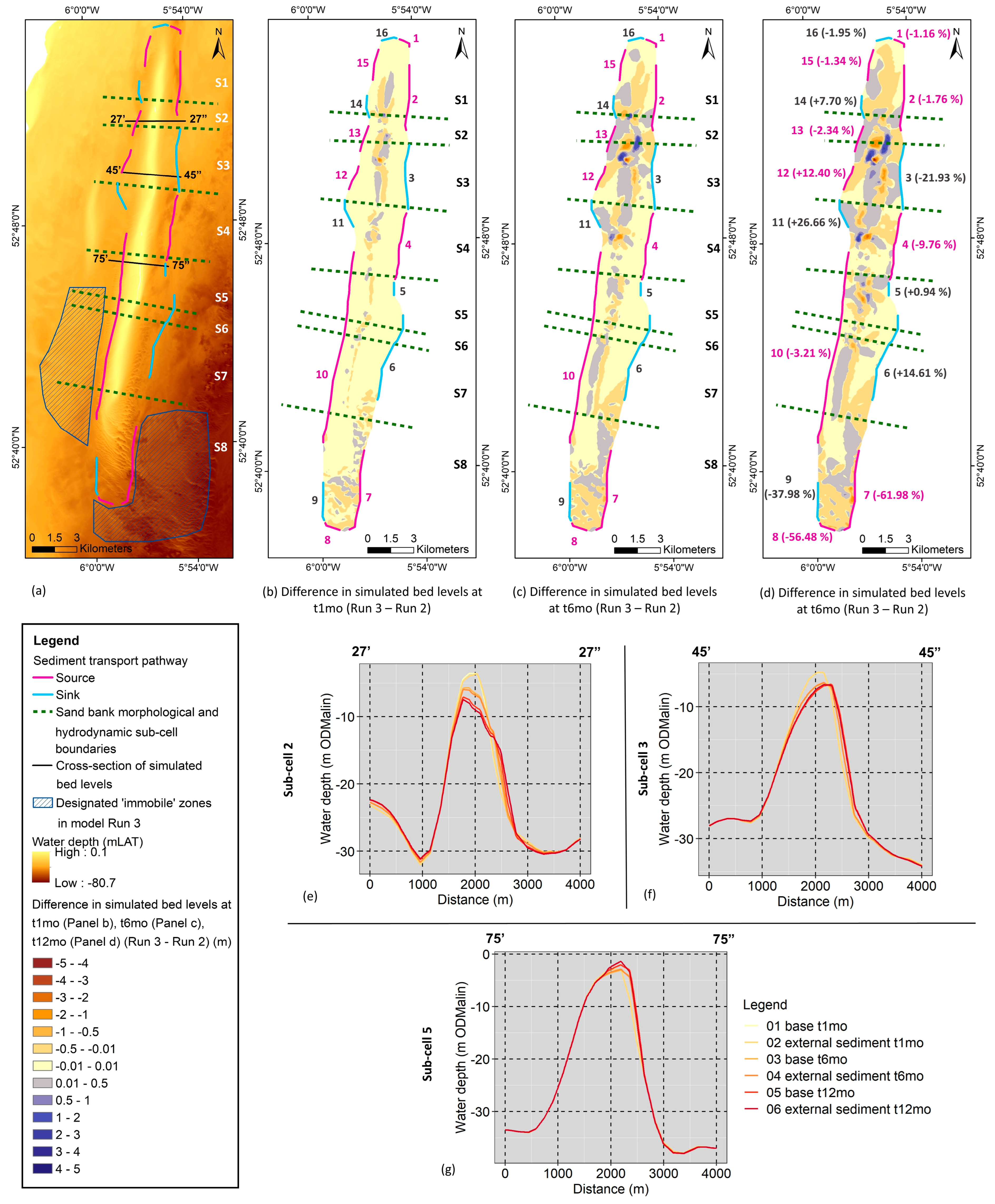
3.3. Influence of External Sediment Sources on Arklow Bank’s Local Sediment Transport Regime

Sediment source pathways 7 and 10 (Figure 11b and Figure 14b) were selected to test the impact of external sediment sources on Arklow Bank’s sediment transport system. These were chosen due to the relatively high portion of external sediment sources they account for in the calculated sediment budget. An area of approximately 46 km² and 29 km² directly outside the morphological cell, opposite pathways 7 and 10, respectively, were designated as immobile zones according to the method outlined in Section 2.2 (Figure 14a). No other variable was changed from the baseline simulation (Run 2) to ensure the impact of this change could be tested accurately.

Results show that the volume change between simulated bed levels within the morphological cell over a one-year period has decreased by 7% compared to baseline calculations. Furthermore, an alteration in the volume of sediment exchanged along the full circumference of the sediment budget cell over this same one-year time period is highlighted (Figure 14d).

Compared to baseline results, a decrease in external sediment entering the morphological cell is most significant at source pathways 7 (−62%), 8 (−56%), and 10 (−3%), whereas a decrease in sediment volume exiting the cell is most notable at sink pathways 3 and 9 by 22% and 38%, respectively. The major reduction in sediment volume passing cross-sections 7, 8, and 9 in Run 3 correlates very well with the adjacent designated ‘immobile’ zones (Figure 14a,d). As less external sediment passes through pathways 7 and 8, this directly reduces the volume of material exported out of the cell via pathway 9.

Figure 14b–g presents bed level differences between Run 2 and Run 3 after one, six, and 12 lunar month simulation periods. These datasets highlight the direct impact of external sediment sources on upper slope bank morphodynamics. Notably, zones of high bed level differences, i.e., high vulnerability zones (HVZs), are identified as early as a one-month simulation, correlating with ‘mobile’ areas of the bank, namely sub-cells 1, 3, 4, 5, and 7 (Figure 14b). Partial overlap with the southern half of the relatively ‘stable’ zone of sub-cell 2 is noted, where the bank transitions from at or above mean sea level (MSL) to a slightly deeper water depth [17]. The slight increase in water depth above the bank crest facilitates a relatively higher quantity and magnitude of residual cross-flow [17] in comparison to the northern half of sub-cell 2. Subsequently, this potentially leaves this area of the bank more vulnerable to other forces such as changes in external sediment sources, wind, and wave-induced flow. However, the bed level changes at the southern tip of the bank, in sub-cell 8, are directly related to changes in sand wave dynamics rather than upper slope morphodynamic changes [15].

After one, six, and 12-month simulation periods, the maximum difference in bed level between Run 2 and Run 3 ranges from +1.29 m to −2.53 m, +3.21 m to −3.56 m, and +2.98 m to −4.85 m, respectively (Figure 14b–d). The most significant HVZs, located in the mid- and northern sections of the bank, align with the change in sediment volume exchanged across pathways 3, 4, 11, 12, 13, and 14. In general, there is an increase in the percentage of sediment transfer on the western side of the bank and a decrease in the percentage of sediment exchanged on the eastern side of the bank in comparison to the baseline run. For example, where the volume of sediment exchanged outwards and inwards increased by 26.66% and 12.4% at pathways 11 and 12, the volume of sediment transported out of pathway 3 decreased by 21.93% (Figure 14d). These correlate with the intersection point of the outer flows of off-bank anticlockwise Eddies D and F on the eastern side of the bank and Eddies E and G on the western side of the bank (Figure 6). This also marks the transition point between bank sub-cells 3 and 4. From Figure 5, the nature of these residual currents differs on either side of this transition zone, yet most notably, the development of on-bank clockwise residual current and residual total load vector eddies at the northern point of sub-cell 4 implies the recycling of sediment between pathways 12 and 11 (Figure 14d).

When comparing cross-sections of simulated bed levels between Run 2 and Run 3 over the identified HVZs, the nature of the change is not consistent in each area. This is most likely due to the complex hydrodynamic and sediment transport systems, which contain:

i.

A high-level clockwise residual circular eddy encompassing the whole bank, caused by flood/ebb tidal dominance, and multiple smaller-scale on-bank clockwise residual eddies, both of which unevenly distribute sediment within the sediment budget cell.

ii.

Multiple anticlockwise residual current and sediment transport eddies, located on the edge of the larger clockwise flow, have the potential to transfer sediment in and out of the cell.

Due to these complex sediment distribution mechanisms, although an overall reduction in volume change is observed between Run 2 and Run 3, changes to the morphodynamics of the bank in each HVZ are inconsistent. For example, along cross-sections L15-L17 and L27–30, a higher magnitude and rate of erosion are observed (Figure 14a–e). Contrastingly, a lower rate of both erosion and mobility is observed in cross-sections L45 to L46 and L52 to L55 (Figure 14a–f), and a higher rate of accretion is notable in cross-sections L75 to L76 (Figure 14a–g). While the maximum range of bed level differences between Run 2 and Run 3 after one, six, and 12 lunar months of simulation is +1.29 m to −2.53 m, +3.21 m to −3.56 m, and +2.98 m to −4.85 m, bed level differences vary between HVZ representative cross-sections (

Table 4. The differences in bed levels between each scenario run along targeted cross-sections over the identified HVZs after a simulation period of 1 month (t1mo), 6 months (t6mo), and 12 months (t12mo). For cross-section locations, see Figure 14a.

Model Run Comparison	Variable	Line ID	T1mo			T6mo			T12mo
			Mean	Max	Min	Mean	Max	Min	Mean	Max	Min
Run 2 Vs. Run 3	Baseline Vs. Changes to external sediment sources	L17	−0.01	0.06	−0.16	−0.03	0.03	−0.21	−0.05	0.03	−0.21
		L27	0.01	0.64	−0.39	0.05	1.3	−0.34	0.05	1.91	−0.61
		L33	0	0.24	−0.23	0.19	1.97	−0.26	0.21	2.35	−0.48
		L45	0	0.02	−0.03	0.01	0.1	−0.05	−0.02	0.27	−0.69
		L63	0	0	−0.05	−0.01	0.01	−0.05	−0.03	0.07	−0.12
		L75	0	0.01	−0.02	−0.01	0.18	−0.43	0	0.67	−0.9
		L77	0	0.01	−0.02	0	0.13	−0.08	−0.06	0.02	−0.66
		L80	0	0.01	−0.02	0	0.01	−0.05	−0.06	0.92	−1.27
		L111	−0.01	0.01	−0.07	−0.04	0.01	−0.4	−0.08	0.07	−0.83
Run 2 Vs. Run 4	Baseline Vs. Addition of Wind and surface pressure	L17	−0.01	0.14	−0.37	−0.01	0.4	−0.91	0.04	0.73	−1.04
		L27	0.04	0.74	−0.19	0.05	1.76	−0.26	0.07	3.03	−0.76
		L33	−0.01	0.25	−0.35	0.17	2.04	−2.33	0.31	2.22	−1.65
		L45	0	0.15	−0.12	−0.01	0.05	−0.04	−0.06	0.33	−0.98
		L63	0.01	0.2	−0.01	−0.02	0.28	−0.21	−0.05	0.81	−0.71
		L75	0	0.04	−0.06	−0.01	0.81	−0.49	−0.05	2.43	−1.35
		L77	0	0.05	−0.08	−0.05	1.32	−1.28	−0.04	4.41	−3
		L80	0	0.04	−0.07	−0.04	0.23	−0.53	−0.14	0.66	−1.8
		L111	0	0.02	−0.03	0	0.15	−0.11	0	0.03	−0.04
Run 2 Vs. Run 5	Baseline Vs. Addition of wind, surface pressure, and wave-induced flow	L17	−0.01	0.17	−0.44	−0.01	0.32	−0.73	−0.05	0.52	−1.02
		L27	−0.01	0.9	−0.52	0.11	2.59	−0.5	0.17	4.65	−1.02
		L33	−0.01	0.3	−0.38	0.12	1.7	−2.79	0.27	2.46	−1.99
		L45	0	0.14	−0.1	−0.02	0.04	−0.06	−0.06	0.32	−0.86
		L63	0.01	0.21	−0.01	−0.02	0.31	−0.23	−0.05	0.92	−0.76
		L75	0	0	−0.02	−0.01	0.44	−0.3	−0.05	1.35	−0.91
		L77	0	0.02	−0.05	−0.03	0.82	−0.71	−0.01	3.98	−2.56
		L80	0	0.03	−0.04	−0.03	0.18	−0.43	−0.03	0.44	−0.46
		L111	0	0.09	−0.07	0.01	0.82	−0.44	0.02	0.78	−0.41
Run 4 Vs. Run 5	Addition of wind and surface pressure Vs. Addition of wind and surface pressure and wave-induced flow	L17	0	0.05	−0.07	−0.01	0.19	−0.21	−0.09	0.05	−0.65
		L27	−0.04	0.16	−0.71	0.06	0.83	−0.25	0.1	1.61	−0.33
		L33	0	0.05	−0.06	−0.06	0.25	−0.77	−0.04	0.92	−0.91
		L45	0	0.02	−0.01	−0.01	0.02	−0.06	0	0.13	−0.08
		L63	0	0.02	0	0	0.03	−0.02	−0.01	0.19	−0.07
		L75	0	0.03	−0.04	0	0.19	−0.37	0.01	0.48	−1.08
		L77	0	0.03	−0.02	0.02	0.57	−0.5	0.03	0.44	−0.46
		L80	0	0.03	−0.01	0.01	0.1	−0.05	0.11	1.64	−0.35
		L111	0	0.07	−0.04	0.01	0.67	−0.33	0.02	0.82	−0.44

). After the first month of simulation, cross-section L17 bed level differences range from +0.06 m to −0.16 m, yet L27 ranges from +0.64 m to −0.39 m. By the 12th simulation month, L17 displays a relatively low difference of +0.03 m to −0.21 m in comparison to L27, which displays a difference of +1.91 m to −0.61 m compared to the base case. Evidently, the range of impact of external sediment sources on bank morphology varies immensely along the bank.

While Coughlan et al. [16] show that the dominant processes controlling seabed disturbance are tidal currents and Creane et al. [17] show that tidal currents are the dominant controlling factor of Arklow Bank’s long-term stability and morphodynamic regime, new analysis ultimately shows that this sedimentary bedform relies on external sediment sources to sustain morphological stability in the existing local sediment transport system.

By introducing a restriction on sediment sources entering the southern part of the bank, a relatively low impact on the one-year bank volume change is revealed. Although the reduction in volume change from Run 2 to Run 3 is quite minimal (7%), the volume of sediment exchanged across each pathway of the entire circumference of the sediment budget cell is modified. Additionally, this reduction in external sediment sources clearly alters the distribution of sediment along the length of the bank, which in turn alters rates and magnitudes of localised erosion/accretion.

This alteration varies along the length of the bank, whereby the areas most impacted are the relatively high mobility areas in the mid- and northern sections of the bank. The visibility of these changes after a single lunar cycle implies that the residual clockwise sediment transport eddy encompassing the bank has the ability to distribute sediment from the southern to the northern extent of the bank over this time frame. This may take place through a combination of bed load and suspended load sediment transport methods. This knowledge could directly apply to other offshore sand banks in tidally-dominated areas. Furthermore, the nature and timeline of this impact imply that a disturbance to the seabed due to anthropogenic processes such as dredging of materials for OWF cable burial or as a source of marine aggregates has the potential to impact erosion and accretion rates and bedform dynamics further along the sediment transport pathway [8]. Similarly, studies have shown that ORE developments alter current and wave propagation [2,4,7,10,12,13,59]. In this way, with the increase in planned anthropogenic activities, a robust marine spatial plan must incorporate a risk assessment that analyses potential changes to the hydrodynamic processes controlling seabed stability identified in this study and in Creane et al. [17]. Ultimately, due to complex local and regional hydrodynamic and sediment transport systems connecting various areas of the south-western Irish Sea [14,15], it is imperative that an assessment be carried out to identify and reduce potential risks to environmental stability both in the immediate and wider area of work. Increasing knowledge of this system and protecting against seabed instability will also reduce risk for ORE developments, protect benthic habitats, protect existing marine commercial industries such as fisheries, and aid marine spatial planning.

A long-term simulation may improve knowledge of the extent and timing of the intricate interconnected sediment transport system. For example, disturbance to the offshore independent sand wave off the eastern side of Arklow Bank, presented in Figure 12, should be tested to understand the dependence of offshore sand deposits on offshore sand banks, the dependence of offshore sand banks on these offshore sand deposits, and the timeline in which this circulatory system exchanges sediment between these two deposition areas. This will ultimately facilitate the development of a robust, sustainable marine spatial plan.

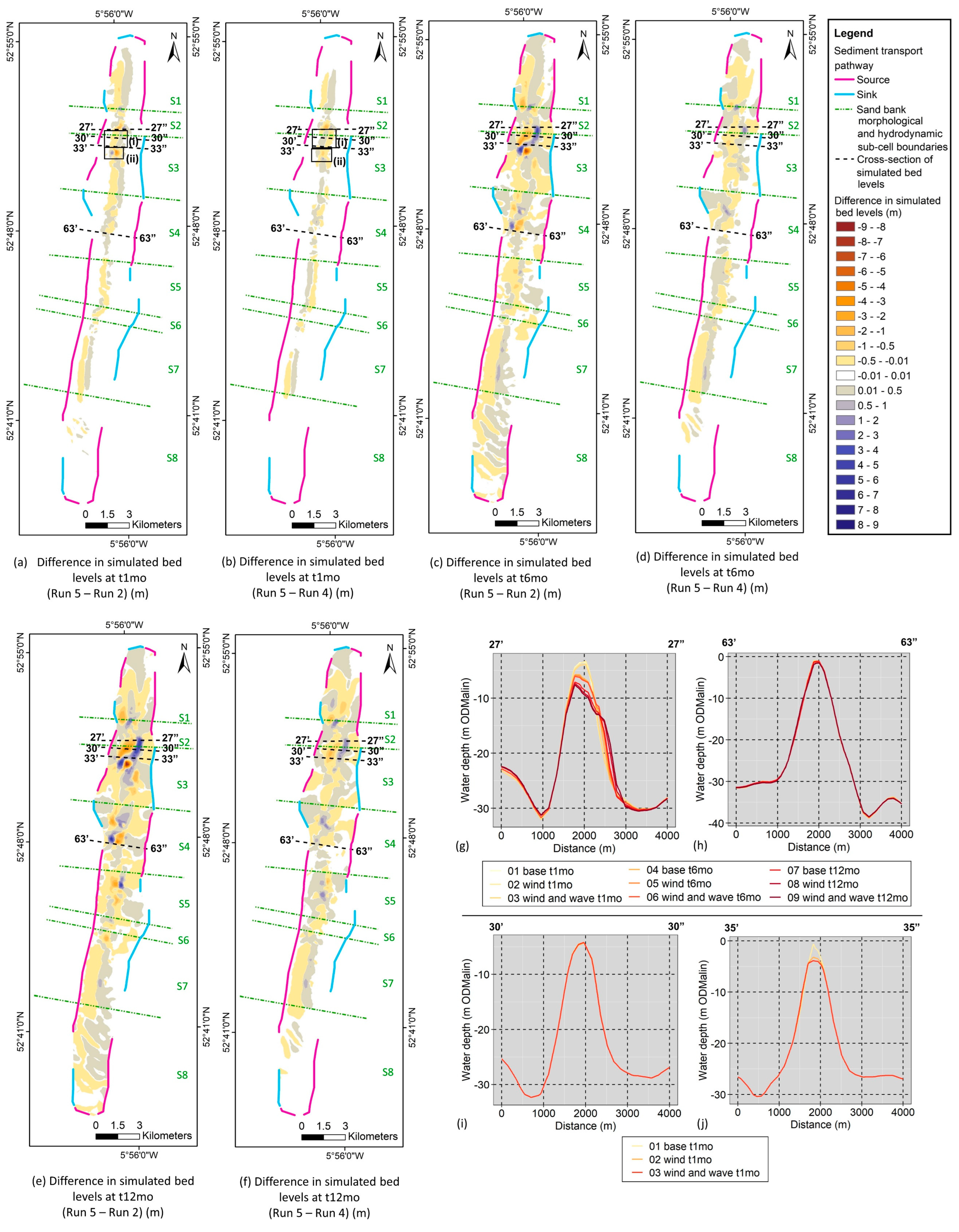
3.4. Impact of Wind on Arklow Bank Morphodynamics

With the inclusion of a wind field in Run 4, high vulnerability zones (HVZs) are identified along the bank. These HVZs are located in the highly dynamic morphological sub-cells 1, 3, 4, and 5 (Figure 15a–d), yet sub-cells 2, 4, 6, 7, and 8 (Figure 15a–d) show very little impact. These vulnerable areas correlate very well with those areas of the bank susceptible to change under the interference of external sediment sources (Section 3.3). Additionally, the areas of stability previously observed in Runs 1 to 3 remain relatively immobile, showing little to no response to wind-induced flow. The maximum difference in simulated bed levels over the whole bank between Run 2 and Run 4 after one, six, and 12 lunar months ranges from +1.37 m to −2.92 m, +5.95 m to −6.90 m, and 6.16 m to −8.32 m, respectively (Figure 15b–d). Notably, this maximum range is not observed in each HVZ (Table 4). For example, cross-sections L33 and L77 represent typical simulated bed-level conditions in these areas (Figure 15f–i). The range of bed level difference between Run 2 and Run 4 after one, six, and 12 lunar months along L33 is +0.25 m to −0.35 m, +2.04 m to −2.33 m, and +2.22 m to −1.65 m, respectively, and along L77 is +0.05 m to −0.08 m, +1.32 m to −1.28 m, and +4.41 m to −3.00 m (Table 4). Notably, in each profile where a difference is noted, it is most significant in the upper slopes, with the highest impact within the upper five metres of the crest (Figure 15f–i).

In shallow environments, wind-induced currents have been shown to both induce surface current velocities and temporally reverse surface current directions [23]. This in turn has a direct impact on sediment transport pathways and morphodynamics, especially bedforms located in relatively shallow water. This study shows that wind-induced currents increase erosion at various HVZs along the bank. This phenomenon is reflected in cross-section L62 (Figure 15a,h), located in sub-cell 4, whereby an increased rate of bed level reduction is evident in comparison to the pure current case. Contrastingly, in other regions, such as over cross-section L39 (Figure 15a,g), a decrease in the rate of bed level reduction is evident. This could be due to a temporary reversal of net current flow in this area or due to sediment resuspension during slack tide and sediment transport in the opposite direction during these slack tidal current conditions, as noted in previous studies in other environments [22,23,24]. This slows this east-west fluctuation behaviour. Subsequent alteration in the timing of the east-west fluctuation of the bank due to this altered flow regime is further visible in cross-section L30 (Figure 15a,e).

Clearly, the magnitude of the altered flow varies depending on the location along the bank and the simulation time step of the extracted bed levels. As the dynamically coupled model includes a morphological feedback loop with simulated hydrodynamics, the bed level is continuously updated. These updated morphological changes are used as a base for flow calculations at the following timestep. In this way, it is difficult to directly compare the direct impact of wind to the baseline bed levels at the 6th and 12th simulated months. Using cross-section L33 as an example (Figure 15a,f), Run 4 bed levels at the 12th lunar month display a bank asymmetry in the opposite direction to baseline bed levels for the same simulation month. The addition of wind-influenced flow continuously modifies the shape of the bank, which ultimately alters the timing of the hydrodynamic-morphodynamic response in the identified vulnerable areas in comparison to the base case. In this way, wind may either accelerate or delay the localised timing of the fluctuation compared to the pure current case.

Although the wind-current interaction implies that shallow areas of the bank should be most influenced by wind-induced flows, this is not always the case here. The relatively stable sub-cells of the bank, namely sub-cells 2 and 6, have crest levels near MSL yet show very little to no impact. On closer examination, the areas mostly impacted align with regions that are relatively shallow (<−5 mMSL) but have an existing relatively high residual cross-flow driving east-west migration of the upper slopes of the bank. The lack of influence of wind on sub-cells 2 and 6 may be due to the absence of a strong residual cross-flow due to the control of wider tidal current phenomena such as off-bank anticlockwise residual eddies and on-bank clockwise eddies [17].

3.5. Impact of Wave-Induced Flow on Arklow Bank Morphodynamics

The areas of the bank impacted by combined current, wave, and wind-induced flow align with those HVZs identified in Section 3.4. The maximum range of bed level difference between Run 5 (current, wind, and wave) and Run 2 (current only) after one, six, and 12 lunar months is +1.65 m to −3.55 m, +5.96 m to −7.34 m, and +7.03 m to −8.71 m (Figure 16a,c,e). However, this maximum range varies across each HVZ over the one-year simulation period, as highlighted in Table 4. For example, the maximum and minimum bed level difference along cross-section L27 (Figure 16g) between Run 5 and Run 2 after one, six, and 12 lunar months is 0.90 m and −0.52 m, 2.59 m and −0.50 m, and 4.65 m and −1.02 m, respectively. However, under the same scenario, L63 (Figure 16h) displays a maximum and minimum bed level difference after one, six, and 12 lunar months of 0.21 m and −0.01 m, 0.31 m and −0.23 m, and 0.92 m and −0.76 m, respectively (Table 4).

Additionally, variation exists between Run 5 and Run 4 (current and wind), where the maximum range of bed level differences after one, six, and 12 lunar months is +1.16 m to −1.52 m, +2.39 m to −1.02 m, and +2.76 m to −1.25 m (Figure 16b,d,f). The variability of this maximum range across each identified HVZ is evident in the extracted representative cross-sections presented in Table 4. In particular, the maximum and minimum bed level difference across L27 (Figure 16g) between Run 5 and Run 4 after one, six, and 12 lunar months is 0.16 m and −0.71 m, 0.83 m and −0.25 m, and 1.61 m and −0.33 m, respectively. However, under the same scenario, L63 (Figure 16h) displays a maximum and minimum bed level difference after one, six, and 12 lunar months of 0.02 m and 0.00 m, 0.03 m and −0.02 m, and 0.19 m and −0.07 m, respectively (Table 4).

Over each HVZ, wave-induced flow is shown to both increase erosion or accretion in comparison to baseline conditions, similar to that shown in [20], which in this case directly correlates with the delay or acceleration of the east-west fluctuation of the upper slopes of the bank (Figure 16a–j, characterised by Creane et al. [17]. This is directly linked to the complex wave-current interaction [60]. Depending on the orientation of wave propagation in relation to the direction of current flow, wave celerity may be increased or decreased [60]. At Arklow Bank, depending on whether wave-induced flow is in the same or opposing direction as tidal currents, the east-west fluctuation of the bank may be delayed or accelerated. Additionally, the general distribution of sediment along the bank may be temporarily altered due to this change.

Furthermore, when analysing the difference between simulated bed levels after one lunar month between (i) Run 5 and Run 2 (Figure 16a) and (ii) Run 5 and Run 4 (Figure 16b), a complex wind-wave interaction is highlighted. For example, in area (i) in Figure 16a, Run 5 displays increased erosion and accretion on the western and eastern sides of the bank, respectively, in comparison to baseline conditions. In area (ii) in Figure 16a, Run 5 displays increased accretion and erosion on the western and eastern sides of the bank in comparison to the baseline model run. By analysing one-month simulated bed levels in these areas from Run 4 to Run 5, the nature of the impact of wind and waves on sediment transport can be isolated. Therefore, when further analysing area (i) together in Figure 16a,b, the addition of wave forcing actually decreases the magnitude of eastward migration of the upper slope in comparison to combined current and wind forcing over this time period (e.g., cross-section L30 in Figure 16a,b,i). However, when analysing area (ii) together in Figure 16a,b, wave forcing increases the rate of westward migration of the upper slope in comparison to combined current and wind forcing over this time period (e.g., cross-section L35) (Figure 16a,b,j). In this way, the addition of wave forcing can further increase or delay the east-west fluctuation of the upper slopes of Arklow Bank. These discrepancies are most likely due to the mis-alignment of the directionality of wind forcing and swell wave propagation. Surface waves can be separated into wind-waves and swell waves. Wind-waves are waves that propagate in the same direction as the wind, whereas swell waves are waves that have been generated elsewhere or before the wind changes direction. In other words, swells are wind-generated waves that are not significantly affected by the local wind at that time. The radiation stresses generated by the spectral wave model for input into Run 5 incorporate both wind-waves and swells. In this way, the mis-alignment in directionality between wind forcing and wave-induced flow has the potential to drive these inconsistent morphodynamic changes. Also, wave refraction, which is the bending of wave energy in shallow water, adds complexity to this interaction.

From this analysis, it is clear that specific areas of the bank are impacted by wind- and wave-tidal current interactions. These phenomena have been shown to either speed up or delay the tidal-current-controlled upper slope east-west fluctuation. However, these forces are not as consistent as tidal currents; instead, they vary over time on an hourly, daily, and seasonal basis. Consequently, the influence they have on bank morphodynamics does not impact the overall long-term behaviour of the bank.

4. Conclusions

This study uses two-dimensional morphological modelling to investigate the extent to which Arklow Bank’s local sediment transport regime is influenced by external sediment sources, wind forcing, and wave forcing. A mesh sensitivity analysis was first carried out to identify the most efficient mesh resolution to investigate various hydrodynamic and morphodynamic processes along the length of the bank. Secondly, a sediment budget was estimated for Arklow Bank in order to analyse the impact of external sediment sources on the local sediment transport regime. Finally, the areas of the bank most vulnerable to wind and wave forcing are identified, and the nature of their impact is revealed. The main outcomes from this study are presented below.

• An unstructured mesh resolution of at least 50 m to 80 m over Arklow Bank is necessary to resolve the timing and nature of the complex east-west fluctuation of the upper slopes of the sand bank. When the mesh resolution over the bank is increased to 150 m to 200 m, the morphological model fails to resolve the timing of this east-west fluctuation but still captures the general hydrodynamic processes controlling both bank base stability and upper slope mobility. Consequently, when considering all variables of a project, such as project objectives, site characteristics, computational time, and project timeline and budget, for a process-understanding study, a coarser resolution model is adequate. However, regardless of the computational time saved by a coarser resolution mesh, to understand the maximum limits of vertical and horizontal bed levels along the length of the bank, a higher resolution mesh is required. The adoption of this criteria is important for studies where a detailed understanding of morphological changes is necessary, such as OWF cable burial depth and scour protection design.
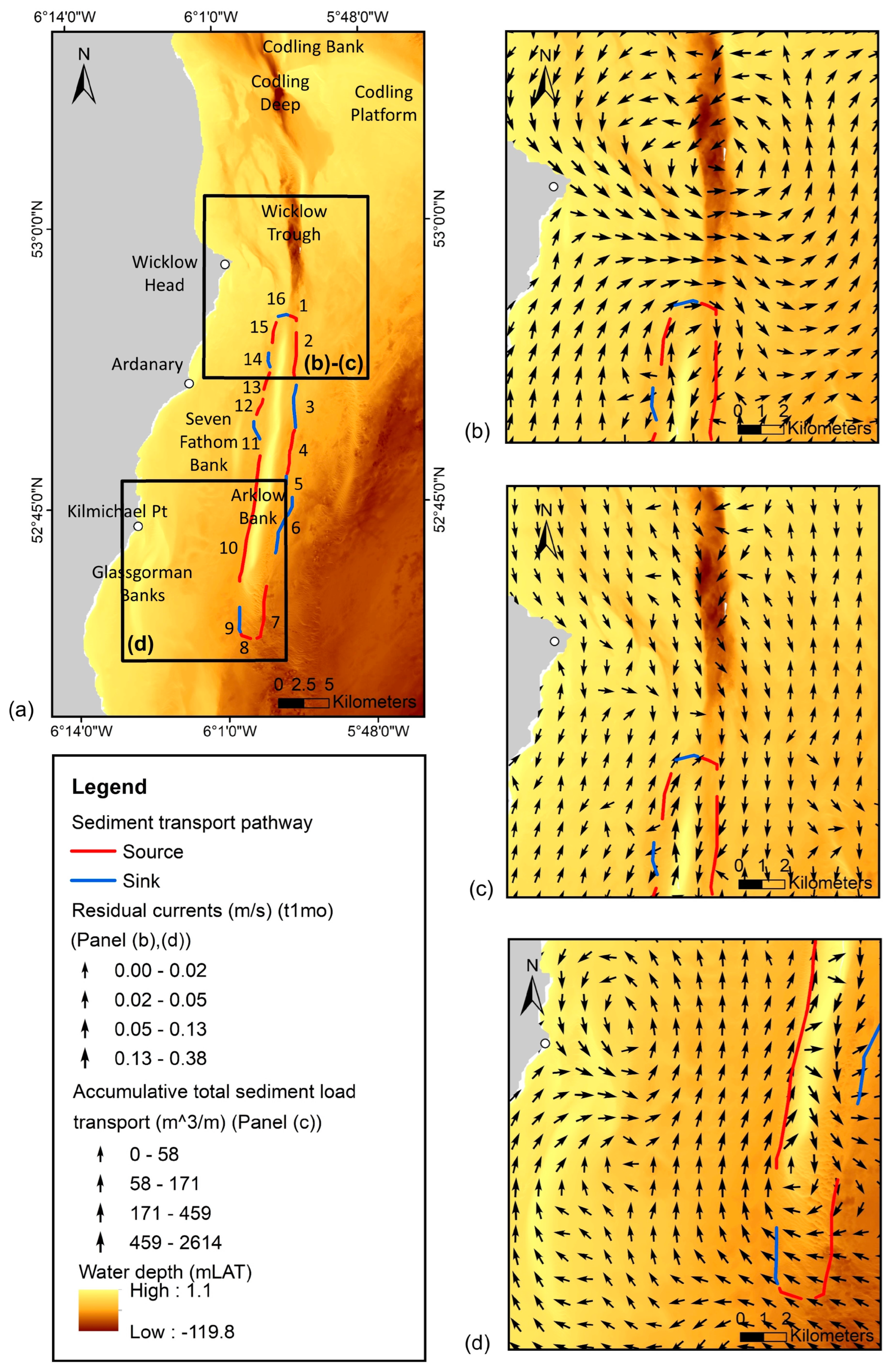
• Using a one-year model simulation, a sediment budget for Arklow Bank is estimated. From this, seven sink and nine source external sediment transport pathways are identified, with the following characteristics:

  (a)

  The identified connection between sink pathways on the eastern side of Arklow Bank and an offshore independent sand wave field 8 km east of Arklow Bank by Creane et al. [15] is further supported here through the identification of SSC residual plumes along the transport pathways and by using a bed load/suspended load dominance factor to support the proposed mechanism of transport.

  (b)

  Sediment sources at the southern extent of the bank are partially connected to the return of sediment from these sand deposits, yet they are also sourced from other offshore sand deposits, including the Glassgorman Banks.

  (c)

  Sediment exchange at the northern extent of Arklow Bank is linked with Wicklow Head and Wicklow Trough, the latter displaying a potential funnelling of sediment from the BLP zone [14].

  (d)

  Finally, the western side of the bank is dominated by sediment exchange between Arklow Bank and Seven Fathom Bank.

• Although sediment distribution along Arklow Bank is mainly due to the large clockwise residual current eddy encompassing the bank, the bank is also influenced by external sediment sources. External sediment exchange is clearly facilitated by the positioning of multiple anticlockwise residual current eddies along the circumference of this main morphological cell [17]. The restriction of sediment sources off the southern extent of the bank leads to changes in erosion and accretion patterns in the mid and northern sections of the bank after just one simulated lunar month. This highlights the short timescale within which the large clockwise residual current eddy distributes sediment throughout the bank. This implies that anthropogenic activities such as dredging for marine aggregates can highly impact areas further along a transport pathway over a relatively short time-scale. The magnitude of this impact depends on the extent and duration of the work. Given the particular complexity of the interconnected sediment transport pathways in the south-western Irish Sea, the risk of seabed instability arising from increased anthropogenic seabed disturbances is high. Robust marine spatial planning that considers these processes is key to reducing the risk of environmental instability.
• The areas of the bank most vulnerable to changes in external sediment sources and the addition of wind and wave forcing are quite consistent. These areas generally align with those regions identified as ‘mobile’ zones in Creane et al. [17] and display a relatively high residual current crossflow under pure current baseline conditions.
• The influence of wind-induced flow on the bank is concentrated in these HVZs. The addition of these forces is shown to both accelerate and reduce the speed of the east-west fluctuation of the upper slopes of the bank.
• The impact of wave-induced flow is also focused on in these HVZs. Although the east-west fluctuation can both accelerate or reduce the speed of the upper slope migration dynamics, it is inconsistent with wind-forcing. This is most likely due to the mis-alignment between wind direction and the directionality of wave-induced flow arising from swell.
• Where tidal currents are the primary control on sediment transport patterns and regulate Arklow Bank morphodynamics, wind and wave forcing are shown to impact vulnerable areas of the system but have a lesser impact on the long-term behaviour of the bank.

References

1. RPS. Arklow Bank Wind Park Phase 2 Offshore Infrastructure: Environmental Impact Assessment Report—Appendix 3.1: Consultation Report; RPS: Abingdon, UK, 2021. [Google Scholar]
2. Auguste, C.; Nader, J.R.; Marsh, P.; Penesis, I.; Cossu, R. Modelling the Influence of Tidal Energy Converters on Sediment Dynamics in Banks Strait, Tasmania. Renew. Energy 2022, 188, 1105–1119. [Google Scholar] [CrossRef]
3. Baeye, M.; Fettweis, M. In Situ Observations of Suspended Particulate Matter Plumes at an Offshore Wind Farm, Southern North Sea. Geo-Mar. Lett. 2015, 35, 247–255. [Google Scholar] [CrossRef]
4. Fairley, I.; Masters, I.; Karunarathna, H. The Cumulative Impact of Tidal Stream Turbine Arrays on Sediment Transport in the Pentland Firth. Renew. Energy 2015, 80, 755–769. [Google Scholar] [CrossRef]
5. Harris, J.M.; Whitehouse, R.J.S.; Sutherland, J. Marine Scour and Offshore Wind—Lessons Learnt and Future Challenges. In Proceedings of the International Conference on Offshore Mechanics and Arctic Engineering—OMAE, Rotterdam, The Netherlands, 19–24 June 2011; Volume 5, pp. 849–858. [Google Scholar] [CrossRef]
6. Lind, R.A.; Whitehouse, R.J.S. Understanding and Assessing Scour Development at Offshore Structures. J. Oilfield Technol. 2012, 5, 63–67. [Google Scholar]
7. Rivier, A.; Bennis, A.-C.; Pinon, G.; Magar, V.; Gross, M. Parameterization of Wind Turbine Impacts on Hydrodynamics and Sediment Transport. Ocean Dyn. 2016, 66, 1285–1299. [Google Scholar] [CrossRef]
8. Demir, H.; Otay, E.N.; Work, P.A.; Börekçi, O.S. Impacts of Dredging on Shoreline Change. J. Waterw. Port Coast. Ocean Eng. 2004, 130, 170–178. [Google Scholar] [CrossRef]
9. Wyns, L.; Roche, M.; Barette, F.; Van Lancker, V.; Degrendele, K.; Hostens, K.; De Backer, A. Near-Field Changes in the Seabed and Associated Macrobenthic Communities Due to Marine Aggregate Extraction on Tidal Sandbanks: A Spatially Explicit Bio-Physical Approach Considering Geological Context and Extraction Regimes. Cont. Shelf Res. 2021, 229, 104546. [Google Scholar] [CrossRef]
10. Clark, S.; Schroeder, F.; Baschek, B. The Influence of Large Offshore Wind Farms on the North Sea and Baltic Sea—A Comprehensive Literature Review (Report No. HZG Report 2014-6); Helmholtz-Zentrum Geesthacht, Zentrum für Material-und Küstenforschung: Geesthacht, Germany, 2014. [Google Scholar]
11. Ivanov, E.; Capet, A.; De Borger, E.; Degraer, S.; Delhez, E.J.M.; Soetaert, K.; Vanaverbeke, J.; Grégoire, M. Offshore Wind Farm Footprint on Organic and Mineral Particle Flux to the Bottom. Front. Mar. Sci. 2021, 8, 631799. [Google Scholar] [CrossRef]
12. Abanades, J.; Greaves, D.; Iglesias, G. Wave Farm Impact on the Beach Profile: A Case Study. Coast. Eng. 2014, 86, 36–44. [Google Scholar] [CrossRef]
13. Onea, F.; Rusu, L.; Carp, G.B.; Rusu, E. Wave Farms Impact on the Coastal Processes—A Case Study Area in the Portuguese Nearshore. J. Mar. Sci. Eng. 2021, 9, 262. [Google Scholar] [CrossRef]
14. Creane, S.; O’Shea, M.; Coughlan, M.; Murphy, J. The Irish Sea Bed Load Parting Zone: Is It a Mid-Sea Hydrodynamic Phenomenon or a Geological Theoretical Concept? Estuar. Coast. Shelf Sci. 2021, 263, 107651. [Google Scholar] [CrossRef]
15. Creane, S.; Coughlan, M.; O’Shea, M.; Murphy, J. Development and Dynamics of Sediment Waves in a Complex Morphological and Tidal Dominant System: Southern Irish Sea. Geosciences 2022, 12, 431. [Google Scholar] [CrossRef]
16. Coughlan, M.; Guerrini, M.; Creane, S.; O’Shea, M.; Ward, S.L.; Van Landeghem, K.J.J.; Murphy, J.; Doherty, P. A New Seabed Mobility Index for the Irish Sea: Modelling Seabed Shear Stress and Classifying Sediment Mobilisation to Help Predict Erosion, Deposition, and Sediment Distribution. Cont. Shelf Res. 2021, 229, 104574. [Google Scholar] [CrossRef]
17. Creane, S.; O’Shea, M.; Coughlan, M.; Murphy, J. Hydrodynamic Processes Controlling Sand Bank Mobility and Long-Term Base Stability: A Case Study of Arklow Bank. Geosciences 2023, 13, 60. [Google Scholar] [CrossRef]
18. Whitehouse, R.J.S.; Harris, J.M.; Sutherland, J.; Rees, J. The Nature of Scour Development and Scour Protection at Offshore Windfarm Foundations. Mar. Pollut. Bull. 2011, 62, 73–88. [Google Scholar] [CrossRef] [PubMed]
19. EMODnet Bathymetry Consortium. EMODnet Digital Bathymetry (DTM 2020). 2020. Available online: https://sextant.ifremer.fr/record/bb6a87dd-e579-4036-abe1-e649cea9881a/ (accessed on 20 March 2020).
20. Giardino, A.; Monbaliu, J. Wave Effects on the Morphodynamic Evolution of an Offshore Sand Bank. J. Coast. Res. SI 2010, 51, 127–140. [Google Scholar] [CrossRef]
21. Idier, D.; Ehrhold, A.; Garlan, T. Morphodynamique d’une Dune Sous-Marine Du Détroit Du Pas de Calais. Comptes Rendus Geosci. 2002, 334, 1079–1085. [Google Scholar] [CrossRef]
22. Mitchell, N.C.; Jerrett, R.; Langman, R. Dynamics and Stratigraphy of a Tidal Sand Ridge in the Bristol Channel (Nash Sands Banner Bank) from Repeated High-Resolution Multibeam Echo-Sounder Surveys. Sedimentology 2022, 69, 1051–1082. [Google Scholar] [CrossRef]
23. Colosimo, I.; de Vet, P.L.M.; van Maren, D.S.; Reniers, A.J.H.M.; Winterwerp, J.C.; van Prooijen, B.C. The Impact of Wind on Flow and Sediment Transport over Intertidal Flats. J. Mar. Sci. Eng. 2020, 8, 910. [Google Scholar] [CrossRef]
24. Daniell, J.J. Bedload Parting in Western Torres Strait, Northern Australia. Cont. Shelf Res. 2015, 93, 58–69. [Google Scholar] [CrossRef]
25. Ulses, C.; Estournel, C.; Durrieu de Madron, X.; Palanques, A. Suspended Sediment Transport in the Gulf of Lions (NW Mediterranean): Impact of Extreme Storms and Floods. Cont. Shelf Res. 2008, 28, 2048–2070. [Google Scholar] [CrossRef]
26. Dan, S.; Vandebroek, E. A Sediment Budget for a Highly Deveoped Coast—Belgian Case. In Proceedings of the Coastal Dynamics 2017, Helsingør, Denmark, 12–16 June 2017; pp. 1376–1385. [Google Scholar]
27. Rosati, J.D. Concepts in Sediment Budgets. J. Coast. Res. 2005, 21, 307–322. [Google Scholar] [CrossRef]
28. Symonds, A.M.; Vijverberg, T.; Post, S.; van der Spek, B.J.; Henrotte, J.; Sokolewicz, M. Comparison between MIKE 21 FM, DELFT3D and DELFT3D FM Flow Models of Western Port Bay, Australia. Coast. Eng. Proc. 2017, 1, 1–12. [Google Scholar] [CrossRef]
29. Li, M.Z.; Hannah, C.G.; Perrie, W.A.; Tang, C.C.L.; Prescott, R.H.; Greenberg, D.A. Modelling Seabed Shear Stress, Sediment Mobility, and Sediment Transport in the Bay of Fundy. Can. J. Earth Sci. 2015, 52, 757–775. [Google Scholar] [CrossRef]
30. Auguste, C.; Marsh, P.; Nader, J.R.; Penesis, I.; Cossu, R. Modelling Morphological Changes and Migration of Large Sand Waves in a Very Energetic Tidal Environment: Banks Strait, Australia. Energies 2021, 14, 3943. [Google Scholar] [CrossRef]
31. Krabbendam, J.; Nnafie, A.; de Swart, H.; Borsje, B.; Perk, L. Modelling the Past and Future Evolution of Tidal Sand Waves. J. Mar. Sci. Eng. 2021, 9, 1071. [Google Scholar] [CrossRef]
32. Leenders, S.; Damveld, J.H.; Schouten, J.; Hoekstra, R.; Roetert, T.J.; Borsje, B.W. Numerical Modelling of the Migration Direction of Tidal Sand Waves over Sand Banks. Coast. Eng. 2021, 163, 103790. [Google Scholar] [CrossRef]
33. Borsje, B.W.; Kranenburg, W.M.; Roos, P.C.; Matthieu, J.; Hulscher, S.J.M.H. The Role of Suspended Load Transport in the Occurrence of Tidal Sand Waves. J. Geophys. Res. Earth Surf. 2014, 119, 701–716. [Google Scholar] [CrossRef]
34. Li, M.Z.; Shaw, J.; Todd, B.J.; Kostylev, V.E.; Wu, Y. Sediment Transport and Development of Banner Banks and Sandwaves in an Extreme Tidal System: Upper Bay of Fundy, Canada. Cont. Shelf Res. 2014, 83, 86–107. [Google Scholar] [CrossRef]
35. Panigrahi, J.K.; Ananth, P.N.; Umesh, P.A. Coastal Morphological Modeling to Assess the Dynamics of Arklow Bank, Ireland. Int. J. Sediment Res. 2009, 24, 299–314. [Google Scholar] [CrossRef]
36. Chatzirodou, A.; Karunarathna, H.; Reeve, D.E. Modelling 3D Hydrodynamics Governing Island-Associated Sandbanks in a Proposed Tidal Stream Energy Site. Appl. Ocean Res. 2017, 66, 79–94. [Google Scholar] [CrossRef]
37. Chatzirodou, A.; Karunarathna, H.; Reeve, D.E. 3D Modelling of the Impacts of In-Stream Horizontal-Axis Tidal Energy Converters (TECs) on Offshore Sandbank Dynamics. Appl. Ocean Res. 2019, 91, 101882. [Google Scholar] [CrossRef]
38. McCarroll, R.J.; Masselink, G.; Valiente, N.G.; Wiggins, M.; Scott, T.; Conley, D.C.; King, E.V. Impact of a Headland-Associated Sandbank on Shoreline Dynamics. Geomorphology 2020, 355, 107065. [Google Scholar] [CrossRef]
39. DHI Group. MIKE 21 Toolbox: User Guide; DHI Group: Hørsholm, Denmark, 2017. [Google Scholar]
40. DHI Group. MIKE 21 Flow Model: Hydrodynamic Module User Guide; DHI A/S: Hørsholm, Denmark, 2017. [Google Scholar]
41. DHI Group. Non-Cohesive Sediment Transport Module—MIKE 21 ST; DHI A/S: Hørsholm, Denmark, 2017. [Google Scholar]
42. Creane, S.; O’Shea, M.; Coughlan, M.; Murphy, J. Estimation of Suspended Solids Concentration from Acoustic Doppler Current Profiler in a Tidally-Dominated Continental Shelf Sea Setting and Its Use as a Numerical Modelling Validation Technique. Coast. Eng. 2022, 14, 53027–53037. [Google Scholar]
43. Engelund, F.; Hansen, E. A Monograph on Sediment Transport in Alluvial Streams; Teknisk Forlag: Copenhagen, Denmark, 1967. [Google Scholar]
44. Wilson, R.J.; Speirs, D.C.; Sabatino, A.; Heath, M.R. A Synthetic Map of the North-West European Shelf Sedimentary Environment for Applications in Marine Science. Earth Syst. Sci. Data 2018, 10, 109–130. [Google Scholar] [CrossRef]
45. DHI Group. MIKE 21 Spectral Waves FM; DHI A/S: Hørsholm, Denmark, 2017. [Google Scholar]
46. Komen, G.J.; Cavaleri, L.; Donelan, M.; Hasselmann, K.; Hasselmann, S.; Janssen, P. Dynamics and Modelling of Ocean Waves; Cambridge University Press: Cambridge, UK, 1994. [Google Scholar] [CrossRef]
47. Young, I.R. Wind Generated Ocean Waves; Elsevier: Amsterdam, The Netherlands, 1999. [Google Scholar]
48. Hasselmann, K. On the Spectral Dissipation of Ocean Waves Due to White Capping. Bound.-Layer Meteorol. 1974, 6, 107–127. [Google Scholar] [CrossRef]
49. Bidlot, J.-R.; Janssen, P.A.E.M.; Abdalla, S. A Revised Formulation of Ocean Wave Dissipation and Its Model Impact. 2007. Available online: https://www.researchgate.net/profile/Jean-Bidlot/publication/256198186_A_revised_formulation_of_ocean_wave_dissipation_and_its_model_impact/links/565429a308aefe619b19ab21/A-revised-formulation-of-ocean-wave-dissipation-and-its-model-impact.pdf (accessed on 25 March 2020).
50. Johnson, H.K.; Kofoed-Hansen, H. Influence of Bottom Friction on Sea Surface Roughness and Its Impact on Shallow Water Wind Wave Modeling. J. Phys. Oceanogr. 2000, 30, 1743–1756. [Google Scholar] [CrossRef]
51. Nikuradse, J. Stromungsgesetze in Rauhen Rohren. J. Appl. Math. Mech./Z. Für Angew. Math. Und Mech. 1931, 11, 409–411. [Google Scholar] [CrossRef]
52. Weber, N. Bottom Friction for Wind Sea and Swell in Extreme Depth-Limited Situations. J. Phys. Oceanogr. 1991, 21, 149–172. [Google Scholar] [CrossRef]
53. Battjes, J.; Janssen, J. Energy Loss and Set-up Due to Breaking of Random Waves. Coast. Eng. Proc. 1978, 1978, 569–587. [Google Scholar] [CrossRef]
54. DHI Group. MIKE 21 Toolbox: Global Tide Model—Tidal Prediction; DHI A/S: Hørsholm, Denmark, 2017. [Google Scholar]
55. Suh, K.D.; Kwon, H.D.; Lee, D.Y. Some Statistical Characteristics of Large Deepwater Waves around the Korean Peninsula. Coast. Eng. 2010, 57, 375–384. [Google Scholar] [CrossRef]
56. Dorschel, B.; Wheeler, A.J. Appraisal of the Irish Sea Seabed Imaging for Tidal Energy Generation Tidal Energy Potential Assessment; INFOMAR Report INF-11-11-WHE; INFOMAR Programme; Geological Survey: Dublin, Ireland, 2012. [Google Scholar]
57. Coughlan, M.; Tóth, Z.; Van Landeghem, K.J.J.; McCarron, S.; Wheeler, A.J. Formational History of the Wicklow Trough: A Marine-Transgressed Tunnel Valley Revealing Ice Flow Velocity and Retreat Rates for the Largest Ice Stream Draining the Late-Devensian British–Irish Ice Sheet. J. Quat. Sci. 2020, 35, 907–919. [Google Scholar] [CrossRef]
58. Coughlan, M.; O’Donnell, E.; Divilly, M.; McCarron, S.; Wheeler, A.J. Irish Sea Tunnel Valleys: Genesis, Development and Present Day Morphology. In Proceedings of the Irish Geological Research Meeting, Galway, Ireland, 19–21 February 2015; Queen’s University Belfast: Belfast, UK, 2015. [Google Scholar] [CrossRef]
59. van Berkel, J.; Burchard, H.; Christensen, A.; Mortensen, L.O.; Svenstrup Petersen, O.; Thomsen, F. The Effects of Offshore Wind Farms on Hydrodynamics and Implications for Fishes. Oceanography 2020, 33, 108–117. [Google Scholar] [CrossRef]
60. USA Corps of Engineers. Coastal Engineering Manual Part II: Coastal Hydrodynamics (EM 1110-2-1100); Books Express Publishing: Berkshire, UK, 2002; Volume 1100.
Figure 2. (ac) shows numerical model boundaries, mesh resolution levels and validation points, whereby (b) specifically displays the four mesh levels used in model runs 2 to 5 and (c) displays the five mesh levels used in model run 1. Panel (a) bathymetry source: EMODnet [19] where MSL is mean sea level; Panel (b) bathymetry source: INFOMAR (https://www.infomar.ie/, accessed on 20 March 2020) where LAT is the lowest astronomical tide. Adapted from Creane et al. [17].
Jmse 11 02027 g002
Figure 3. Three sediment sample datasets were used in this study’s sediment transport model: (i) in situ surficial sediment samples; (ii) synthetic samples from Wilson et al. [44]; and (iii) artificial samples derived from the cross-correlation of in situ samples with multi-beam echo-sounder data and/or existing regional scale sediment distribution maps. Numerical model mesh boundary levels are illustrated.
Jmse 11 02027 g003
Figure 4. Wave model validation plots: (ac) time-series plots of significant wave height ( H s ), spectral zero-crossing wave period ( T 02 ) and mean wave direction ( M W D ) at M2 data point; (df) time-series plots of H s , T 02 and M W D at M5 data point; (gj) scatter plots of H s at M2, M5, ERA5 1 and ERA5 2 data point locations. The coordinates of each data point are provided in Table 1.
Jmse 11 02027 g004
Figure 5. Diagram displaying Arklow Bank hydro- and morpho-dynamics under pure current conditions produced by Creane et al. [17]. Adapted from Creane et al. [17].
Jmse 11 02027 g005
Figure 6. (a,b) display residual currents calculated after the first lunar month simulation from Run 1 and Run 2, respectively (Table 2). The approximate location of the centre point of each off-bank anticlockwise residual eddy and two on-bank clockwise residual eddies, originally identified in Creane et al. [17], is provided in each figure. Bathymetry source: INFOMAR (https://www.infomar.ie/ (accessed on 20 March 2020)).
Jmse 11 02027 g006
Figure 7. (a) Location of Arklow Bank in the south-western Irish Sea; (b) Difference in simulated bed levels between Run 1 and Run 2 at the starting model timestep (t0); (c) Difference in simulated bed levels between Run 1 and Run 2 after a 12 lunar month simulation period (t12mo). Bathymetry source: INFOMAR (https://www.infomar.ie/ (accessed on 20 March 2020)).
Jmse 11 02027 g007
Figure 8. Cross-sectional analysis of simulated bed levels of Run 2 against Run 1 in identified ‘stable’ zones: (bi) display simulated bed level over a one-year simulation at cross-sections 23, 65, 67, and 92, whereby ‘t0′ is the starting bed level and ‘h’, ‘wk’, and ‘mo’ are subsequent months; (a) provides the location of these cross-sections. Bathymetry source: INFOMAR (https://www.infomar.ie/ (accessed on 20 March 2020)).
Jmse 11 02027 g008
Figure 9. Cross-section L65 (b) displays a comparison of bed levels between interpolated INFOMAR bathymetry using the higher and lower resolution unstructured triangular meshes used in Run 1 and Run 2, respectively, against baseline INFOMAR survey data. (a) displays the location of this cross-section. Bathymetry source: INFOMAR (https://www.infomar.ie/ (accessed on 20 March 2020)).
Jmse 11 02027 g009
Figure 10. Cross-sectional analysis of simulated bed levels of Run 2 against Run 1 in identified ‘mobile’ zones. (bm) display simulated bed level over a one-year simulation at multiple cross-sections, whereby ‘t0′ is the starting bed level and ‘h’, ‘wk’, and ‘mo’ are subsequent months; (a) provides the location of these cross-sections. Bathymetry source: INFOMAR (https://www.infomar.ie/ (accessed on 20 March 2020)).
Jmse 11 02027 g010
Figure 11. (a) Bathymetry map overlain by simulated accumulative total sediment load transport vectors after a 12-month simulation period. The identified source and sink pathways are identified along the circumference of the sediment budget cell in red and blue, respectively. (b) The percentage of the total sediment entering the sediment budget cell through each source pathway over this 12-month period is presented in red. The percentage of the total sediment exiting the sediment budget cell at each sink pathway over this 12-month period is identified in blue. Bathymetry source: INFOMAR (https://www.infomar.ie/ (accessed on 20 March 2020)).
Jmse 11 02027 g011
Figure 12. (a) Bathymetry (mLAT) overlain by modelled residual currents (m/s); (b) Mean simulated SSC (g/m3) over a one-year period under pure current conditions overlain by modelled residual currents (m/s); (c) Bed load versus suspended load dominance calculated from one lunar month simulation under pure current conditions overlain by modelled residual currents (m/s). Bathymetry source: INFOMAR (https://www.infomar.ie/ (accessed on 20 March 2020)).
Jmse 11 02027 g012
Figure 13. (a) Identified sink and source pathways around Arklow Bank’s sediment budget cell in relation to the Wicklow Trough and Wicklow Head; (b) Simulated residual currents, after the first simulation month (t1mo), over Wicklow Trough and Northern Arklow Bank; (c) Modelled accumulative total sediment load over, after a 12 lunar month simulation, over Wicklow Trough and Northern Arklow Bank; (d) Simulated residual currents t1mo over Glassgorman Banks and Arklow Bank. Bathymetry source: INFOMAR (https://www.infomar.ie/ (accessed on 20 March 2020)).
Jmse 11 02027 g013
Figure 14. (a) Identified sediment sink and source pathways on the circumference of Arklow Bank’s sediment budget cell. Each morphological sub-cell identified in Creane et al. [17] is labeled; for example, ‘S1′ refers to ‘sub-cell 1′. The locations of simulated bed-level cross-sections are given. Areas designated as ‘immobile zones’ in Run 3 are also denoted. (bd) Difference in simulated bed levels after one (t1mo), six (t6mo), and 12 (t12mo) lunar month simulations between Run 2 and Run 3, respectively (Table 4). (d) also displays the percent total sediment load volume change between Run 3 and Run 2 at each source and sink transport pathway (see (eg) Cross-sections of simulated bed levels after one (t1mo), six (t6mo), and 12 (t12mo) lunar month simulations between Run 2 and Run 3, respectively). Panel (a) bathymetry source: INFOMAR (https://www.infomar.ie/ (accessed on 20 March 2020)).
Jmse 11 02027 g014
Figure 15. (a) Identified sediment sink and source pathways on the circumference of Arklow Bank’s sediment budget cell. The locations of simulated bed-level cross-sections are given. (bd) Difference in simulated bed levels after one (t1mo), six (t6mo), and 12 (t12mo) lunar month simulations between Run 2 and Run 4, respectively (Table 4). (ei) Cross-sections of simulated bed levels after one (t1mo), six (t6mo), and 12 (t12mo) lunar month simulations between Run 2 and Run 4, respectively. Panel (a) bathymetry source: INFOMAR (https://www.infomar.ie/ (accessed on 20 March 2020)).
Jmse 11 02027 g015
Figure 16. (a,c,e) Difference in simulated bed levels after one (t1mo), six (t6mo), and 12 (t12mo) month simulation periods, respectively, between Run 2 and Run 5; (b,d,f) Difference in simulated bed levels after one, six, and 12 month simulation periods, respectively, between Run 4 and Run 5 (see Table 4); (gj) Cross-sections of simulated bed levels from Run 2 (‘base’), Run 4 (‘wind’), and Run 5 (‘wind and wave’).
Jmse 11 02027 g016