Spatiotemporal Variations of Ocean Upwelling and Downwelling Induced by Wind Wakes of Offshore Wind Farms

Abstract

Offshore wind farms (OWFs) generate large-scale wind wakes, which might lead to upwelling/downwelling. Understanding the vertical marine response to the wake effects is crucial for assessing the ecological impacts of OWFs and optimizing their co-deployments with mariculture. In this study, we employ a high-resolution ocean model to investigate the spatiotemporal variations of upwelling and downwelling induced by the wind wakes of OWFs through idealized numerical experiments. We have two main findings. First, the wind-wake-induced upwelling and downwelling are not balanced in the north–south direction, resulting in a net effect of thermocline rising. Second, the thermocline depth changes caused by wind wakes develop nonlinearly over time. Specifically, when the elevated thermocline approaches the sea surface, the upwelling slows down significantly. The spatially asymmetric pattern of the upwelling is attributed to horizontal Ekman transport, while its temporal nonlinear evolution is caused by stratification changes. By utilizing the simulated change law of thermocline depth, we calculate the ocean response of OWF wakes in China’s adjacent waters. The results suggest that baroclinic theory overestimates the ocean response in the Bohai Sea, the Yellow Sea, and the nearshore waters of the East China Sea. However, in the open seas and the South China Shelf, the upwelling/downwelling is expected to be close to the theoretical calculations. This study provides a foundation for conducting regional simulations with high resolutions in areas where OWFs will be constructed.

1. Introduction

Global climate change currently poses a significant threat to human survival and progress. To avert climate disasters, it is imperative to cease emitting greenhouse gas, which serves as the primary driver of climate change. Renewable energy must play a paramount role in mitigating emissions while simultaneously sustaining rapid and extensive economic development. Wind energy (WE) holds a prominent position among renewable energy sources. Compared to onshore WE, offshore wind energy (OWE) has higher abundance [1] due to its larger dimensions and enhanced efficiency [2]. There is an anticipated surge of 130 GW in new capacity for OWE over the next five years (2023–2027), which will increase the offshore wind market’s share of total new global installations from the current 11% to 23% by 2027 [3].

The current phase of rapid development and immense growth in OWE exploitation necessitates an urgent investigation of the environmental impacts of offshore wind farms (OWFs) [4]. From an ecological perspective, OWFs may affect bird populations through collisions and the alteration of migration patterns [5]. The noise generated by OWFs disrupts fish communication [6,7]. OWFs can also function as artificial reefs and aggregation sites for benthic fish [8]. The presence of OWFs significantly changes the nutrient flow and system structure in coastal ecosystems, with both positive and negative effects on various organisms [9] and alterations in local productivity [10]. In terms of dynamics, OWFs cause alterations in wave energy and ocean currents [11]. They introduce additional turbulence into the water, acting as artificial mixing sources [12], thereby influencing ocean mixing and vertical stratification [11,13]. Importantly, wind turbine arrays reduce wind speed as a result of wind wake on the downstream side of OWFs [14,15]. Wind wakes can cause up to a 40% reduction in wind speed [16,17], with their observed length exceeding 70 km [18]. The magnitude and length of these reductions are regulated by the atmospheric stability, turbulence intensity, boundary layer, and turbine performance [19,20,21,22].

The wind wake effect serves as a bridge between the dynamical and ecological impacts of OWFs [23]. According to Ekman’s theory [24], wind wakes of OWFs can cause significant vertical movements in the ocean beneath them. Conducting towed surveys in the leeward regions of operational OWFs yielded empirical evidence of the presence of such movements [25]. Therefore, OWFs have the potential to generate artificial upwelling, thereby pumping nutrients into the euphotic layer. This process enhances ocean carbon storage capacity and increases marine carbon sinks [26]. The co-deployment of OWFs, marine ranching, and marine culture farms is attractive to developers due to the possibility of intensive space and energy utilization [27,28]. The upwelling induced by OWFs has the potential to fertilize jointly operated marine culture.

Regarding the wind wakes of OWFs, most studies focused on wind fields [29]. For example, optimizing wind turbine layout can reduce wake effects and increase power production [30,31]. The OWF wake effect has also been studied in relation to regional and global meteorology [32,33]. There are fewer investigations addressing the ocean response. Using a simplistic analytical model, Broström found that wind wakes of OWFs theoretically induce upwelling exceeding 1 m per day [34]. Estimation using this analytical model has been conducted for China’s adjacent waters [35]. The simplified theory laid the foundations of the study of the impact of OWFs on marine stratifications; however, it fails to capture the detailed spatiotemporal variations in the oceanic dynamic response. This is because the impacts of background currents and boundary constrains on the target phenomenon are absent in their theory.

High-resolution simulations are needed to capture the comprehensive process of upwelling/downwelling. Previous studies indicate that the existence of horizontal wind gradients has the potential to initiate Ekman pumping [36]. Furthermore, the wind forcing can lead to the formation of vortex streets and overturning flow in the wake regions of the OWFs, as indicated by numerical simulation [37]. Some results revealed significant changes in vertical velocities for different OWF designs, including turbine placement, rotor size, and hub height [38], as well as in response to surface gravity waves [39]. Upwelling is found to be spatially variational using numerical models of atmospheric and ocean circulation [40]. Wind farms can also affect the wave field. It has been observed that the difference in wind speed between the coupled simulation utilizing the Weather Research and Forecasting (WRF) and Simulating WAves Nearshore (SWAN) models and the uncoupled simulation utilizing only the WRF model can exceed ±20% [41]. The utilization of the Semi-implicit Cross-scale Hydroscience Integrated System Model (SCHISM) has revealed the emergence of large-scale dipoles in OWF regions, with spatial dimensions reaching hundreds of kilometers [42].

From these studies, it seems that we know little about the net vertical transport of water beneath wind wakes. Additionally, the nonlinear temporal evolution of oceanic thermocline depth in response to wind wakes is still unknown. Given the vast potential of OWF development in China’s adjacent seas, it is especially essential to panoramically estimate the wind wake effects of OWFs, including the impact on upwelling and downwelling. It is impractical to use a high-fidelity model, with spatial resolutions of, e.g., 10⁰ m~10¹ m, to cover all of the water adjacent to China. Therefore, using idealized simulations to verify and revise the simplistically theoretical estimation is more realistic.

This paper investigates the impact of wind wakes on oceanic upwelling and downwelling, with a particular emphasis on analyzing their spatiotemporal variations and underlying mechanisms. A numerical model with fine spatial resolutions is used to diagnose the net vertical transport of water and its temporal evolution. The estimation is utilized to examine potential thermocline depth changes induced by the wind wakes of OWFs in China’s adjacent seas. The data and methods are described in Section 2. In Section 3, we analyze and discuss the results and identify the associated mechanism. Finally, the conclusions are presented in Section 4.

2. Methodology and Data

2.1. Numerical Model

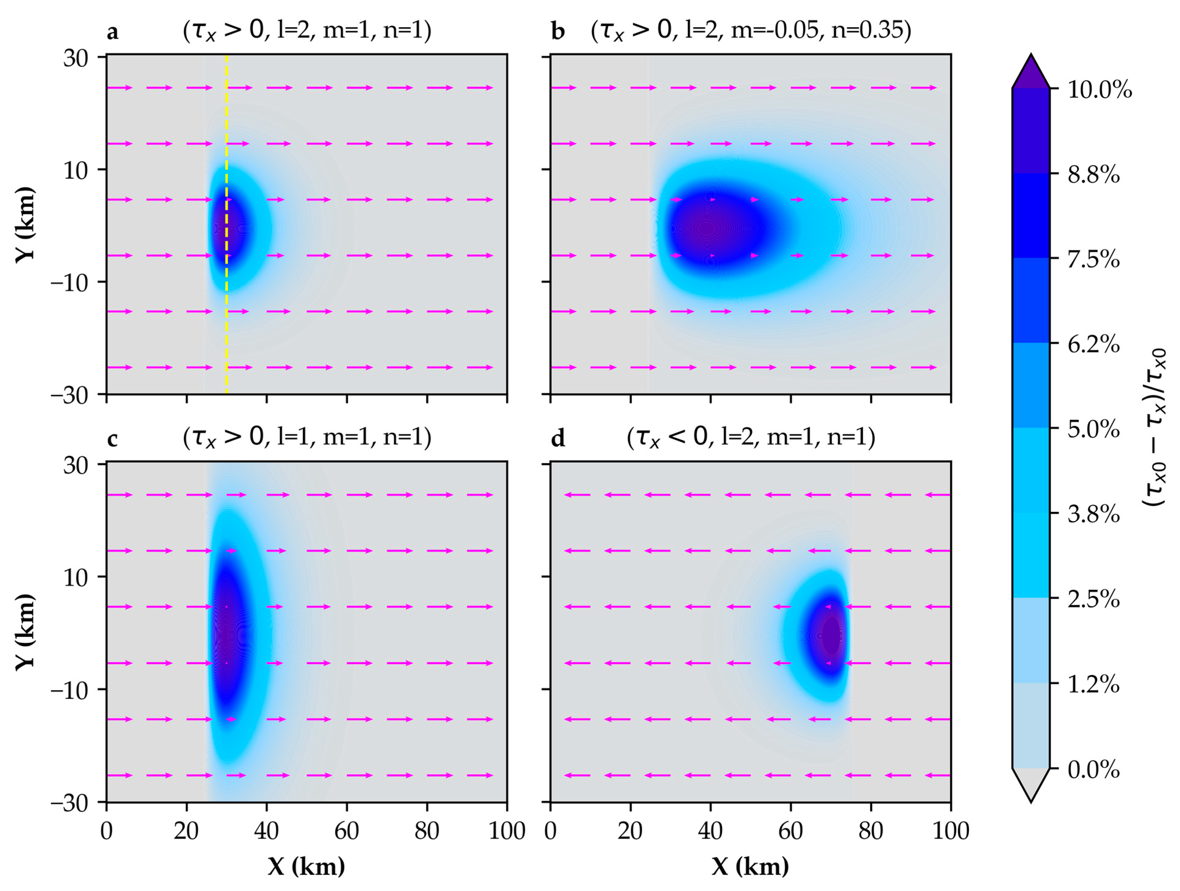
To investigate the dynamic response of the upper ocean to the wind wakes of OWFs, we conducted a series of idealized experiments using the Regional Ocean Modeling System (ROMS). ROMS (software available at https://www.myroms.org/) is a widely used three-dimensional numerical model capable of accurately simulating complex ocean processes, including fluid dynamics and biogeochemistry. The simulation area had dimensions of 100 km × 100 km horizontally, with a fixed water depth of 20 m. The horizontal resolution was set to 400 m × 400 m, and the vertical resolution was 0.5 m. A constant Coriolis parameter (f) 1.39 × 10⁻⁴ s⁻¹ was used.

We employed a combination of periodic boundary conditions, and the salinity was uniformly set to 30 practical salinity units (PSU). The temperature above the thermocline’s upper boundary is denoted as $T_1$, and below its lower boundary ($h_0$) as $T_2$. Within the thermocline, the temperature decreases linearly from $T_1$ to $T_2$, and the total depth of the thermocline is 0.5 m. In the primary experiment (Exp. A), we configured $T_1$ to 20 °C (from 0 to 4.75 m), $T_2$ to 10 °C (from 5.25 to 20 m), and $h_0$ to 5.25 m.

To isolate the influence of wakes, the simulations were divided into two scenarios: without and with wakes. We also separated the scenario involving wakes into two phases. The simulation was initially run for 15 days with spatially homogenous initial wind stress ($\tau$), which represents the shear stress exerted by the wind on the water surface. The wind field with a wake was then used in the simulation for the final 30 days.

2.2. Wind Wake

We designed artificial wind wakes and used those to force the ocean in the simulation. The wind wakes were oriented in the X-direction, with an expansion in the Y-direction. To investigate the impact of wind wake shapes, we explored several simple forms of wind wake that could be represented by the following expressions, which were adapted from the work of Broström (2008) [34]:

$${\tau }_x={\tau }_{x0}-\mathsf{\Delta }{\tau }_x{e}^{-{\left(\frac{ly}{4+0.2x}\right)}^2}\times \max \left(0,e^{m-nx}x\right),$$

(1)

Here, ${\tau }_x$ represents the wind stress in the X-direction, ${\tau }_{x0}$ denotes the wind stress outside OWFs, and $\mathsf{\Delta }{\tau }_x$ reflects the maximum wind stress deficit caused by OWFs. We used various values of the two parameters in the simulations. We also use a set of three parameters ($l, m, n$) in Equation (1) to describe the length and width of the wake. $l$ and $n$ determine the range of the wind wake in the Y- and X-directions. Smaller values of $l$ or $n$ result in larger wake ranges in the Y- or X-directions. $m$ indicates the extent of wind stress reduction. $x$ is a dimensionless number, and it denotes the relative location in the X-direction. Figure 1 illustrates the shapes of the wind wakes and the values of the parameters. Notice that in Figure 1d, ${\tau }_x$ is negative (i.e., the orientation of the wake is in the opposite direction to those in Figure 1a–c).

2.3. Design of the Experiments

To investigate the dynamic effects of OWFs on the ocean under different conditions, a series of idealized numerical experiments (Exp. A–H) were conducted, as outlined in

Table 1. Configurations of the experiments.

Exp.	Wake Shape	${\mathit{\tau }}_{\mathit{x}0}\left|\mathsf{\Delta }{\mathit{\tau }}_{\mathit{x}}\right(\mathit{N}·{\mathit{m}}^{-2})$	${\mathit{h}}_0\left(\mathit{m}\right)$	${\mathit{T}}_1\left|{\mathit{T}}_2\right(\mathbf{°}\mathbf{C})$	Description
A	Figure 1a	0.05|0.005	5.25	20|10	Reference
B	Figure 1a	0.06|0.006	5.25	20|10	High wind stress
C	Figure 1a	0.05|0.01	5.25	20|10	High wind reduction
D	Figure 1a	0.05|0.005	5.25	20|15	Weak stratification
E	Figure 1a	0.05|0.005	10.25	20|10	Deep thermocline
F	Figure 1d	−0.05|−0.005	10.25	20|10	East wind
G	Figure 1b	0.05|0.005	5.25	20|10	Long wake
H	Figure 1c	0.05|0.005	5.25	20|10	Wide wake

. It should be noted that Exp. C has a loss rate ($\mathsf{\Delta }{\tau }_x/{\tau }_{x0}$) of 20%, although the shape of the wind wakes in Figure 1a was used.

2.4. Acquisition of Thermocline Bathymetry and Wind Field Data

Based on numeric simulations, we revised the simple theoretical estimations of the effects of OWFs in China’s adjacent waters. Our study focused on the region between 105°–127.5° E longitude and 15°–41° N latitude. We obtained the initial thermocline depth data from the temperature data in the World Ocean Atlas (WOA) dataset, specifically the WOA 2023 quarterly average dataset spanning from 1991 to 2020, with a resolution of 0.25° [43]. In the designated region, a range of water depths spanning from 10 m to 300 m was chosen, and the position of the thermocline was calculated. The site exhibiting the most robust average temperature gradient was chosen based on a minimum continuous temperature gradient of less than −0.05 °C/m and a thickness exceeding 5 m [44]. The wind product of QSCAT/NCEP [45] was utilized in our evaluation to obtain wind stress (Section 3.5).

2.5. Theoretical Upwelling/Downwelling

In a barotropic ocean, the Ekman pumping velocity ($w_E$) can be expressed as:

$$w_E=\frac{1}{\rho f}\left(\frac{\partial {\tau }_y}{\partial x}-\frac{\partial {\tau }_x}{\partial y}\right),$$

(2)

Here, $\rho$ represents the seawater density, $f$ is the Coriolis parameter, and ${\tau }_y$ is the wind stress in the Y-direction. Forced by the wind wake in Exp. A, $w_E$ exhibits a north–south symmetry in space, as shown in Figure 2. Overall, the south side experiences upwelling, while the north side exhibits downwelling, with velocities reaching up to 0.25 m/day.

In the case of the baroclinic ocean, the vertical velocity ($w_{bc}$) is regulated by the presence of stratification. Following the work of Broström (2008) [34], all processes of short time scales ($t<1/f$, such as internal gravity waves and geostrophic adjustment process) and the temporal changes in wind forcing are neglected. Thus, the maximum $w_{bc}$ is roughly given by:

$$w_{bc}=h\left(a^2\right)\times \frac{\mathsf{\Delta }\mathsf{\tau }}{\rho fL},$$

(3)

where $h\left(a^2\right)$ is a function of $a^2$, and its form is provided by the numeric solution obtained by Broström (2008) [34]. $a=\sqrt{g^{\prime }{h}_0}/fL$, where $\sqrt{g^{\prime }{h}_0}/f$ is the baroclinic Rossby radius and L is the length of the front row of OWFs, perpendicular to the wind direction. $\mathsf{\Delta }\tau$ is the total wind stress deficit. We uniformly set L to 5 km in this study. Additionally, $g\prime =g\Delta \rho /\rho$ is the reduced gravity, and $\Delta \rho$ is the density changes between the upper and the lower ocean. In Exp. A, the maximum $w_{bc}$ is 0.31 m/day, according to this theory. The vertical velocity from the baroclinic theory (Equation (3)) will be examined in comparison with numerical results and the revised equation in Section 3.2 and Section 3.5, respectively.

3. Results

We investigated the vertical and horizontal variation in the simulated upwelling/downwelling by comparing the simulations with the theoretical estimations of Equation (3). Additionally, we presented the temporal evolution of thermocline depth and provided dynamic analyses to understand the mechanisms associated with net upwelling and nonlinear thermocline depth changes.

3.1. Vertical Temperature Anomalies

The wake-induced temperature anomalies (TAs) in the vertical section (from an overhead perspective, the section is delineated by the yellow line as depicted in Figure 1a) are shown in Figure 3. Here, TAs are obtained by subtracting the undisturbed initial temperature from the results of Exp. A. The positive/negative TA values indicate that the water temperature is warmer/colder than normal due to the presence of wind farm wake.

The distribution of TAs exhibits a north–south asymmetry. Negative anomalies dominate the southern section, while positive anomalies are prevalent in the northern counterpart. Negative TAs are primarily concentrated near the thermocline depth, while positive TAs are predominantly observed below the thermocline. Compared to negative TAs, positive TAs can extend far away from the thermocline. Furthermore, the cores of TAs differ. The extreme positive TAs are generally located at the geometric center, whereas the core of the negative TA shifts southward over time.

The rates of TA change over time. Initially, they change rapidly and then gradually slow down. By the 10th day, the extreme TAs reach 2.89 °C and −2.99 °C, respectively. After 30 days, they further increase to 4.51 °C and −4.59 °C, respectively. The slowing down of TAs can be attributed to the weakening of stratification induced by vertical seawater mixing. The reduced vertical temperature difference leads to a decrease in vertical heat transport, which is closely related to the rates of TA.

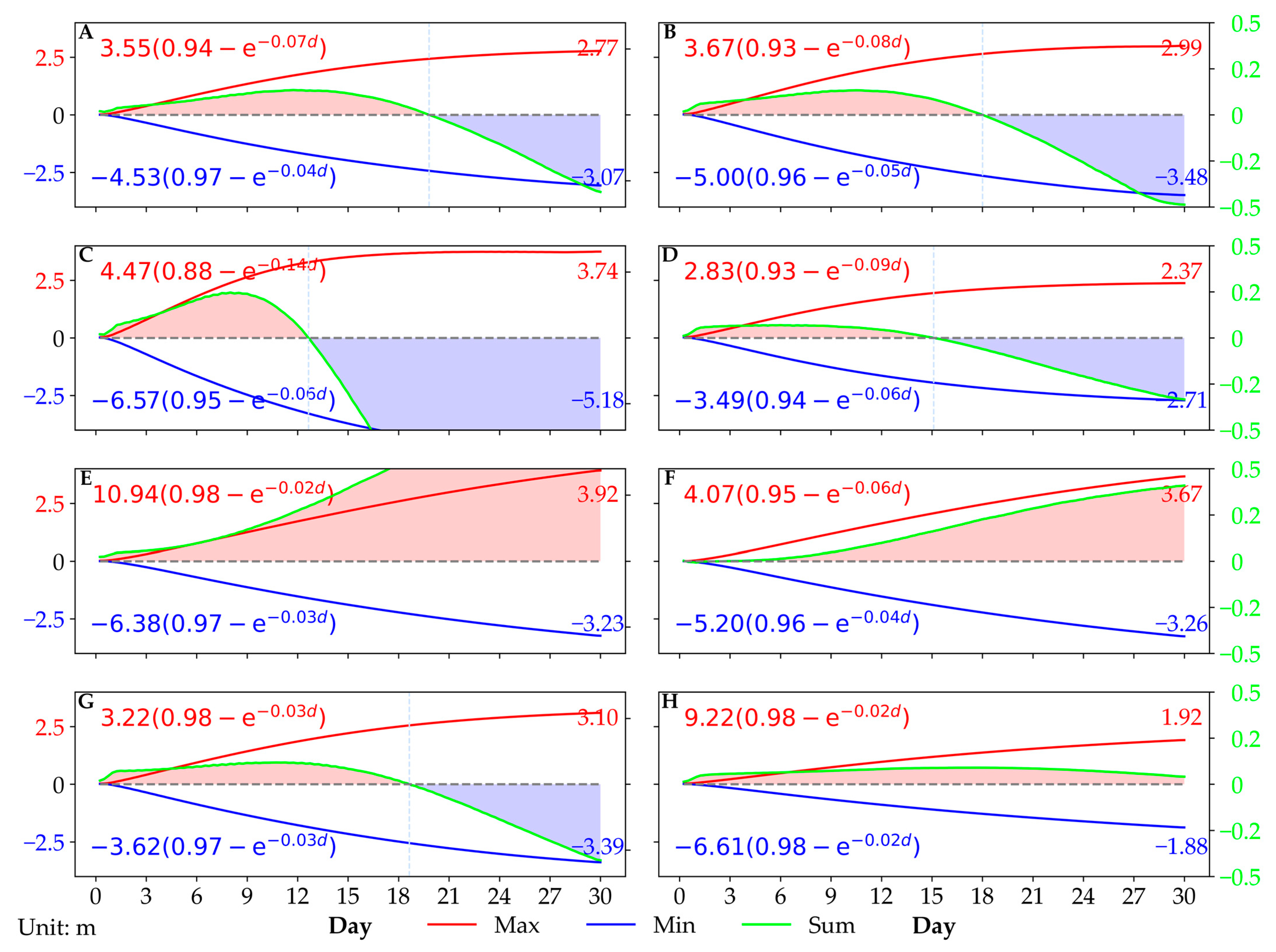
3.2. Changes in Thermocline Depth

Following Broström (2008) [34], we introduced $∆H_{ml}$ to examine the changes in thermocline depth:

$$∆H_{ml}=h_0-\frac{1}{T_1-T_2}{\int }_{-H}^0\left(T-T_2\right)dz,$$

(4)

Here, $T$ represents the depth-dependent temperature, while $H$ is water depth. Equation (4) indicates that $∆H_{ml}$ is positive when thermocline rises, and vice versa.

Figure 4 illustrates the spatiotemporal variations of $∆H_{ml}$. Overall, the southern thermocline rises, while the northern thermocline sinks. In terms of spatial pattern, the upwelling zone is wider than the downwelling zone, with the thermocline rising area being approximately 20% larger than the sink zone. The temporal evolution of the thermocline depth change shows a nonlinear behavior, particularly for thermocline rising. Initially, the rising is more substantial compared to the sinking. By the 15th day, the vertical displacements reach 2.06 m and −1.98 m, respectively. Five days later, they become comparable at about $\pm$2.42 m. Eventually, the maximum rising and sinking reach 2.77 m and −3.07 m, respectively. This result is significantly less than the barotropic estimation (0.25 m × 30 days = 7.5 m) and the baroclinic estimation (0.31 m × 30 days = 9.3 m).

3.3. Comparisons of the Results from Different Experiments

Significant differences are observed in the maximum thermocline rising (red lines in Figure 5) and sinking (blue lines in Figure 5) among the simulations using different configurations (Table 1). We take Exp. A as the control experiment (Figure 5A). In this experiment, positive $∆H_{ml}$ (upwelling) is larger than the negative (downwelling) before the 20th day, after which the negative becomes larger than the positive $∆H_{ml}$. Moreover, $∆H_{ml}$ exhibits a nonlinear evolution, starting with a fast rate, which slows down gradually.

The presence of spatially unbalanced positive and negative $∆H_{ml}$ suggests the occurrence of a net upwelling effect, which is evident in the initial stages of all experiments. In the experiments with deep thermoclines (Figure 5E,F), the positive $∆H_{ml}$ is constantly more prominent than the negative $∆H_{ml}$ throughout the entire simulation. It is noteworthy that, similar to eastward wind (all experiments except for Exp. F), westward wind can also generate net upwelling (Figure 5F). This implies that the presence of a net upwelling is not wind-direction-dependent, and the net upwelling is expected to occur on the right side of the wind.

Regarding temporal evolutions, the nonlinearity is evident in all simulations expected for the deep thermocline set (Figure 5E,F). In these two experiments, the thermocline rates remain almost constant over time. Similarly, the rate forced by a wide wake is nearly linear (Figure 5H), albeit with a small magnitude. The results suggest that the linear changes in thermocline depth are modulated by the sea surface boundary when the thermoclines are close to the surface.

Each experiment requires a specific investigation. In the experiment with large wind stress (Figure 5B), the features are essentially the same as those of Exp. A but with a larger magnitude. The increase in $∆H_{ml}$ is roughly proportional to the increase in wind stress. In Exp. C (large wind stress deficit, Figure 5C), $∆H_{ml}$ changes rapidly, and a larger maximum $∆H_{ml}$ is observed. Weakened stratifications lead to fewer extrema of $∆H_{ml}$ (Figure 5D). It should be noted that the signs of net $∆H_{ml}$ reverse early in Exp. C and Exp. D, indicating a relatively fast rate of $∆H_{ml}$. When the thermoclines are deep, the positive extrema of $∆H_{ml}$ are significantly larger (Figure 5E,F). Upwelling dominates the ocean response, whether forced by eastward or westward winds. The effect of a long wake (Figure 5G) is not notably different compared to the controlled experiment, whereas a wide wake induces a weaker ocean response (Figure 5H).

3.4. Mechanisms of the Spatially Net $∆H_{ml}$ and the Nonlinearity of $∆H_{ml}$ Evolution

To understand the mechanisms behind the spatial distribution of net $∆H_{ml}$ and the nonlinearity of its evolution due to changes in the wind field induced by OWFs, various time-averaged properties derived from Exp. A, such as sea level height anomaly (Z), temperature (T), vertical velocity (W), Brunt-Väisälä frequency (N), and horizontal velocity (U and V), were examined and are presented in Figure 6. These phenomena were a result of changes in the wind field induced by OWFs, as explained earlier in the text. With the exception of the time-averaged N, which was computed over the last 12 days, all other properties were time-averaged over the preceding 18 days. N is described by the following equation:

$$N={\left(-\frac{g}{{\rho }_0}\frac{d\rho }{dz}\right)}^{\frac{1}{2}},$$

(5)

where $g$ is the gravitational acceleration, ${\rho }_0$ is the equilibrium density, and $d\rho /dz$ is the change in density with height.

The positive net $∆H_{ml}$ is attributed to the southward Ekman transport. In the northern region, downwelling leads to water subduction, which is then transported southward. This process leads to horizontal volume convergence in the southern region of the wake, eventually enhancing upwelling here. The reason for the spatially unbalanced $∆H_{ml}$ is illustrated in Figure 7. The reversal of wind direction leads to upwelling/downwelling occurring in the north/south, while the Ekman transport also reverses northward. Despite these changes, the positive $∆H_{ml}$ remains more prominent than the negative $∆H_{ml}$, as verified in the experiments with eastward winds (Exp. F).

The nonlinearity of $∆H_{ml}$ evolution is mainly governed by the gradual increase of N. Affected by the upwelling, simulations demonstrate that N is more significant in the upper layer than in the lower layer, indicating high vertical stability in the upper ocean. A stable ocean is capable of slowing down the rate of $∆H_{ml}$, as demonstrated in the comparison between Exp. A and Exp. D.

3.5. Implications in China’s Adjacent Waters

Based on the analysis above, it is evident that the theory (Equation (3)) overestimates the wind wake impacts. This is because the upwelling is temporally constant based on Equation (3), but the rates of the thermocline rising/falling gradually slow down according to the simulations. To improve the estimation in China’s adjacent waters, we revised the baroclinic estimation. As suggested by the numeric experiments, the upwelling slows down when the thermoclines approach the sea surface. We assumed that the velocity of the upwelling ($W\prime$) can be expressed by $W^{\prime }=r_{0}r{w}_{bc}$, where $w_{bc}$ is the estimation from the baroclinic theory, $r$ is a thermocline-depth-dependent modification factor, and $r_0$ is a constant to represent the difference between the theoretical estimation and the simulated upwelling. When the thermocline is deep, the difference is small, so $r_0$ is close to 1. By observing the simulations, we designed a function of $r$:

$$r\left(h\right)=\left\{\begin{array}{cc}0& h<3.8\\ A{h}^2+Bh+C& 3.8\le h<8.8\\ 1& 8.8\le h\end{array}\right.,$$

(6)

where h is thermocline depth in meters. $A$, $B$ and $C$ are three undetermined coefficients. They were obtained by fitting a simulation which were as same as Exp. A, except for $h_0=10.25$ m. We used $A=-0.018$, $B=0.431$, and $C=-1.373$ in the following analysis. The fitted curve of $r\left(h\right)$ and the simulated $r$ can be seen in Figure 8. We set $r_0=0.727,$ as suggested by the simulations.

The theoretical estimations of the thermocline depth changes and the revision based on simulations are demonstrated in Figure 9. Using gridded temperature and wind data (averaged in June, July, and August), we calculated $w_{bc}$ based on Equation (3), then obtained the theoretical estimations for the maximum $\mathsf{\Delta }{H}_{ml}$ within one month by multiplying $w_{bc}$ by 30. The revised estimations were obtained by modifying the theoretical $\mathsf{\Delta }{H}_{ml}$ based on Equation (6). Firstly, it shows that the high $\mathsf{\Delta }{H}_{ml}$ is mainly concentrated in the nearshore waters of Zhejiang and Jiangsu. The other highly impacted area is the Taiwan Strait, as well as the areas located to the northwest of the Bohai Sea. The theoretical maximum $\mathsf{\Delta }{H}_{ml}$ is higher than 4 m. On the contrary, the outcomes of the model revision exhibit a notable disparity when compared to the estimates derived from the baroclinic theory. This discrepancy is particularly pronounced in regions characterized by high $\mathsf{\Delta }{H}_{ml}$, where the differences exceed 3 m. The majority of areas exhibit disparities of approximately 1 m (Figure 9c). Figure 9d,e illustrate the number of days required for the thermoclines to ascend by 1.5 m. In the nearshore waters of Zhejiang and Jiangsu, as well as in the Taiwan Strait and the Bohai Sea, the model revision lags behind the pure theoretical estimations by almost 10 days in the time needed (Figure 9f). Considering that the theoretical estimation is less than 20 days in these regions (Figure 9d), the relative differences from two estimations are significant. This is the combined result of the active upwelling and the shallow thermoclines (Figure 10) in these regions.

4. Discussions

It should be noted that although Exp. A–H use a fixed water depth of 20 m, this parameter is enough to be used to analyze the target phenomenon. On the one hand, offshore wind power installations are predominantly located in shallow water areas [4]. On the other hand, the results of our numerical experiments indicate that when the thermocline is deep, its vertical velocity is close to the theoretical estimations (Figure 9, r~1, when h > 8.8). Consequently, the revised thermocline depth changes in the surrounding seas adjacent to China are reasonable.

This study explores the upwelling/downwelling dipole prompted by OWFs. The fundamental pattern of the dipole structure aligns with the previous studies based on both the ocean general circulation model [34] and the unstructured grid model [42]. Some in situ observations have demonstrated large-scale structural change in the stratification strength surrounding OWFs, indirectly affirming the potential impacts predicted by the theory and simulation. However, there remains a notable absence of long-term measurements of seawater vertical velocity beneath the wind wakes of OWFs. Further investigation is required to fully comprehend these target impacts.

The net upwelling induced by wind wakes is likely to play an essential role in regulating the marine ecosystem around OWFs. The upwelling transports nutrients from deep seawater to the surface, promoting marine ecosystem productivity. These nutrients are essential for the growth of phytoplankton and contribute to carbon sequestration in the ocean. More importantly, these nutrients facilitate the operations of MCFs. The colocations of OWFs and MCFs have the potential to promote the growth of seaweed and shellfish via the ecological enhancement induced by the upwelling, thus improving economic benefits. A joint operation of the energy and culture sectors should take full advantage of the upwelling and avoid disadvantages associated with the downwelling. It should be noted that the net upwelling occurs on the right side of the prevailing wind direction in the northern hemisphere.

Some phenomena associated with the wind wake effect have not been included in this study. For example, the wind wake is constant in time. Air–sea coupling simulations are necessary to conduct detailed investigations regarding the integrated process. Additionally, we did not focus on wave and tidal effects associated with wind wakes in this study. A model combined with the wave, tide, and ecological modules will be conducted in the future to fill the gap.

5. Conclusions

This study confirms that OWFs have a significant impact on ocean stratification. Wind wakes induced by OWFs are capable of generating upwelling or downwelling. The basic pattern of the marine response aligns with the barotropic and barocline theory. However, the simulation reveals that the changes in thermocline depth due to the wake effect has obvious nonlinear spatiotemporal variations, which cannot be represented by the theoretical estimations. The physical mechanisms of the variations can be explained as follows: On the one hand, the horizontal Ekman transport is responsible for the spatially unbalanced thermocline depth changes. Thus, the integrated effect of wind wakes is net upwelling. On the other hand, the changes in stratification from upwelling suppress the thermocline rising as it approaches the sea surface. These two counterparts interact with each other, leading to a nonlinear ocean response evolution.

This study provides an estimation of the wind wake effect on marine stratifications in China’s adjacent waters. For the regions studied, such as the Bohai Sea, Yellow Sea, nearshore waters of the East China Sea, and the Taiwan Strait, baroclinic theory overestimates the target marine response. According to the theory, the thermoclines ascend to the surface within 30 days. On the contrary, the maximum thermocline changes revised by the simulations are less than 1.5 m in these areas. In the open seas of the Yellow Sea, the East China Sea, and the South China Shelf, the simulations are close to the theoretical calculations.

The study provides insights into the environmental effects of OWFs. It lays the foundations for conducting regional simulations with high resolutions at the specific bays or waters where OWFs are going to be constructed. The estimations can be used to design the marine observation scheme, together with data calibration and verification.

References

1. Bilgili, M.; Yasar, A.; Simsek, E. Offshore wind power development in Europe and its comparison with onshore counterpart. Renew. Sustain. Energy Rev. 2011, 15, 905–915. [Google Scholar] [CrossRef]
2. Li, Y.; Huang, X.; Tee, K.F.; Li, Q.; Wu, X.-P. Comparative study of onshore and offshore wind characteristics and wind energy potentials: A case study for southeast coastal region of China. Sustain. Energy Technol. Assess. 2020, 39, 100711. [Google Scholar] [CrossRef]
3. Global Wind Energy Council. GWEC Global Wind. Report. 2023; Global Wind Energy Council: Brussels, Belgium, 2023. [Google Scholar]
4. Bailey, H.; Brookes, K.L.; Thompson, P.M. Assessing environmental impacts of offshore wind farms: Lessons learned and recommendations for the future. Aquat. Biosyst. 2014, 10, 8. [Google Scholar] [CrossRef]
5. Furness, R.W.; Wade, H.M.; Masden, E.A. Assessing vulnerability of marine bird populations to offshore wind farms. J. Environ. Manag. 2013, 119, 56–66. [Google Scholar] [CrossRef] [PubMed]
6. Kikuchi, R. Risk formulation for the sonic effects of offshore wind farms on fish in the EU region. Mar. Pollut. Bull. 2010, 60, 172–177. [Google Scholar] [CrossRef]
7. Wahlberg, M.; Westerberg, H. Hearing in fish and their reactions to sounds from offshore wind farms. Mar. Ecol. Prog. Ser. 2005, 288, 295–309. [Google Scholar] [CrossRef]
8. Öhman, M.C.; Malm, T.; Wilhelmsson, D. The influence of offshore windpower on demersal fish. ICES J. Mar. Sci. 2006, 63, 775–784. [Google Scholar] [CrossRef]
9. Wang, J.; Zou, X.; Yu, W.; Zhang, D.; Wang, T. Effects of established offshore wind farms on energy flow of coastal ecosystems: A case study of the Rudong offshore wind farms in China. Ocean. Coast. Manag. 2019, 171, 111–118. [Google Scholar] [CrossRef]
10. Slavik, K.; Lemmen, C.; Zhang, W.; Kerimoglu, O.; Klingbeil, K.; Wirtz, K.W. The large-scale impact of offshore wind farm structures on pelagic primary productivity in the southern North Sea. Hydrobiologia 2018, 845, 35–53. [Google Scholar] [CrossRef]
11. van Berkel, J.; Burchard, H.; Christensen, A.; Mortensen, L.; Petersen, O.; Thomsen, F. The Effects of Offshore Wind Farms on Hydrodynamics and Implications for Fishes. Oceanography 2020, 33, 108–117. [Google Scholar] [CrossRef]
12. Schultze, L.K.P.; Merckelbach, L.M.; Horstmann, J.; Raasch, S.; Carpenter, J.R. Increased Mixing and Turbulence in the Wake of Offshore Wind Farm Foundations. J. Geophys. Res. Ocean. 2020, 125, e2019JC015858. [Google Scholar] [CrossRef]
13. Carpenter, J.R.; Merckelbach, L.; Callies, U.; Clark, S.; Gaslikova, L.; Baschek, B. Potential Impacts of Offshore Wind Farms on North Sea Stratification. PLoS ONE 2016, 11, e0160830. [Google Scholar] [CrossRef]
14. Christiansen, M.B.; Hasager, C.B. Wake effects of large offshore wind farms identified from satellite SAR. Remote Sens. Environ. 2005, 98, 251–268. [Google Scholar] [CrossRef]
15. Porté-Agel, F.; Wu, Y.-T.; Chen, C.-H. A Numerical Study of the Effects of Wind Direction on Turbine Wakes and Power Losses in a Large Wind Farm. Energies 2013, 6, 5297–5313. [Google Scholar] [CrossRef]
16. Dong, G.; Li, Z.; Qin, J.; Yang, X. How far the wake of a wind farm can persist for? Theor. Appl. Mech. Lett. 2022, 12, 100314. [Google Scholar] [CrossRef]
17. Platis, A.; Siedersleben, S.K.; Bange, J.; Lampert, A.; Barfuss, K.; Hankers, R.; Canadillas, B.; Foreman, R.; Schulz-Stellenfleth, J.; Djath, B.; et al. First in situ evidence of wakes in the far field behind offshore wind farms. Sci. Rep. 2018, 8, 2163. [Google Scholar] [CrossRef]
18. Hasager, C.B.; Vincent, P.; Husson, R.; Mouche, A.; Badger, M.; Peña, A.; Volker, P.; Badger, J.; Di Bella, A.; Palomares, A.; et al. Comparing satellite SAR and wind farm wake models. J. Phys. Conf. Ser. 2015, 625, 012035. [Google Scholar] [CrossRef]
19. Méchali, M.; Barthelmie, R.; Frandsen, S.; Jensen, L.; Réthoré, P.-E. Wake effects at Horns Rev and their influence on energy production. In Proceedings of the European Wind Energy Conference and Exhibition, Athens, Greece, 27 February–2 March 2006; pp. 10–20. [Google Scholar]
20. Pérez, C.; Rivero, M.; Escalante, M.; Ramirez, V.; Guilbert, D. Influence of Atmospheric Stability on Wind Turbine Energy Production: A Case Study of the Coastal Region of Yucatan. Energies 2023, 16, 4134. [Google Scholar] [CrossRef]
21. Barthelmie, R.J.; Churchfield, M.J.; Moriarty, P.J.; Lundquist, J.K.; Oxley, G.S.; Hahn, S.; Pryor, S.C. The role of atmospheric stability/turbulence on wakes at the Egmond aan Zee offshore wind farm. J. Phys. Conf. Ser. 2015, 625, 012002. [Google Scholar] [CrossRef]
22. Fischereit, J.; Brown, R.; Larsén, X.G.; Badger, J.; Hawkes, G. Review of Mesoscale Wind-Farm Parametrizations and Their Applications. Bound. Layer Meteorol. 2021, 182, 175–224. [Google Scholar] [CrossRef]
23. Gonzalez-Rodriguez, A.G.; Serrano-Gonzalez, J.; Burgos-Payan, M.; Riquelme-Santos, J. Multi-objective optimization of a uniformly distributed offshore wind farm considering both economic factors and visual impact. Sustain. Energy Technol. Assess. 2022, 52, 102148. [Google Scholar] [CrossRef]
24. Beesley, D.; Olejarz, J.; Tandon, A.; Marshall, J. A Laboratory Demonstration of Coriolis Effects on Wind-Driven Ocean Currents. Oceanography 2008, 21, 72–76. [Google Scholar] [CrossRef]
25. Floeter, J.; Pohlmann, T.; Harmer, A.; Moellmann, C. Chasing the offshore wind farm wind-wake-induced upwelling/downwelling dipole. Front. Mar. Sci. 2022, 9, 16. [Google Scholar] [CrossRef]
26. Pan, Y.; Fan, W.; Zhang, D.; Chen, J.; Huang, H.; Liu, S.; Jiang, Z.; Di, Y.; Tong, M.; Chen, Y. Research progress in artificial upwelling and its potential environmental effects. Sci. China Earth Sci. 2015, 59, 236–248. [Google Scholar] [CrossRef]
27. Michler-Cieluch, T.; Krause, G.; Buck, B.H. Marine Aquaculture within Offshore Wind Farms: Social Aspects of Multiple-Use Planning. Gaia 2009, 18, 158–162. [Google Scholar] [CrossRef]
28. Aryai, V.; Abbassi, R.; Abdussamie, N.; Salehi, F.; Garaniya, V.; Asadnia, M.; Baksh, A.A.; Penesis, I.; Karampour, H.; Draper, S.; et al. Reliability of multi-purpose offshore-facilities: Present status and future direction in Australia. Process. Saf. Environ. Prot. 2021, 148, 437–461. [Google Scholar] [CrossRef]
29. González-Longatt, F.; Wall, P.; Terzija, V. Wake effect in wind farm performance: Steady-state and dynamic behavior. Renew. Energy 2012, 39, 329–338. [Google Scholar] [CrossRef]
30. Pryor, S.C.; Barthelmie, R.J.; Shepherd, T.J. Wind power production from very large offshore wind farms. Joule 2021, 5, 2663–2686. [Google Scholar] [CrossRef]
31. Yang, K.; Kwak, G.; Cho, K.; Huh, J. Wind farm layout optimization for wake effect uniformity. Energy 2019, 183, 983–995. [Google Scholar] [CrossRef]
32. Baidya Roy, S. Can large wind farms affect local meteorology? J. Geophys. Res. 2004, 109, D19101. [Google Scholar] [CrossRef]
33. Golbazi, M.; Archer, C.L.; Alessandrini, S. Surface impacts of large offshore wind farms. Environ. Res. Lett. 2022, 17, 064021. [Google Scholar] [CrossRef]
34. Broström, G. On the influence of large wind farms on the upper ocean circulation. J. Mar. Syst. 2008, 74, 585–591. [Google Scholar] [CrossRef]
35. Lian, Z.; Liu, K.; Yang, T. Potential Influence of Offshore Wind Farms on the Marine Stratification in the Waters Adjacent to China. J. Mar. Sci. Eng. 2022, 10, 1872. [Google Scholar] [CrossRef]
36. Pickett, M.H.; Paduan, J.D. Ekman transport and pumping in the California Current based on the U.S. Navy’s high-resolution atmospheric model (COAMPS). J. Geophys. Res.-Ocean. 2003, 108, 3327. [Google Scholar] [CrossRef]
37. Paskyabi, M.B. Offshore Wind Farm Wake Effect on Stratification and Coastal Upwelling. Energy Procedia 2015, 80, 131–140. [Google Scholar] [CrossRef]
38. Segtnan, O.H.; Christakos, K. Effect of Offshore Wind farm Design on the Vertical Motion of the Ocean. Energy Procedia 2015, 80, 213–222. [Google Scholar] [CrossRef]
39. Paskyabi, M.B.; Fer, I. Upper Ocean Response to Large Wind Farm Effect in the Presence of Surface Gravity Waves. Energy Procedia 2012, 24, 245–254. [Google Scholar] [CrossRef]
40. Raghukumar, K.; Nelson, T.; Jacox, M.; Chartrand, C.; Fiechter, J.; Chang, G.; Cheung, L.; Roberts, J. Projected cross-shore changes in upwelling induced by offshore wind farm development along the California coast. Commun. Earth Environ. 2023, 4, 116. [Google Scholar] [CrossRef]
41. Fischereit, J.; Larsén, X.G.; Hahmann, A.N. Climatic Impacts of Wind-Wave-Wake Interactions in Offshore Wind Farms. Front. Energy Res. 2022, 10, 881459. [Google Scholar] [CrossRef]
42. Christiansen, N.; Daewel, U.; Djath, B.; Schrum, C. Emergence of Large-Scale Hydrodynamic Structures due to Atmospheric Offshore Wind Farm Wakes. Front. Mar. Sci. 2022, 9, 818501. [Google Scholar] [CrossRef]
43. Locarnini, R.A.; Baranova, O.K.; Mishonov, A.V.; Boyer, T.P.; Reagan, J.R.; Dukhovskoy, D.; Seidov, D.; Garcia, H.E.; Bouchard, C.; Cross, S.; et al. World Ocean Atlas 2023, Volume 1: Temperature. A. Mishonov Technical Ed. NOAA Atlas NESDIS. 2023; in preparation. Available online: https://www.ncei.noaa.gov/access/world-ocean-atlas-2023/ (accessed on 4 May 2023).
44. Hao, J.; Chen, Y.; Wang, F.; Lin, P. Seasonal thermocline in the China Seas and northwestern Pacific Ocean. J. Geophys. Res. Ocean. 2012, 117, C02022. [Google Scholar] [CrossRef]
45. QSCAT/NCEP Blended Ocean Winds from Colorado Research Associates (Version 5.0). Available online: http://rda.ucar.edu/datasets/ds744.4/ (accessed on 4 October 2021).
Figure 1. Wind wakes used in the simulations. (a) Main wind wake distribution: l = 2 , m = 1 , n = 1 , and τ x > 0 . (b) Long wind wake distribution: m = 0.05 , n = 0.35 , with other parameters identical to (a). (c) Wide wind wake distribution: l = 1 , with other parameters as in (a). (d) Same wind wake distribution as in (a) except for the wind direction ( τ x < 0 ) . The yellow line in (a) denotes the center of the wake at X = 30 km, which will be used for the subsequent cross-sectional analysis.
Jmse 11 02020 g001
Figure 2. Distribution of vertical velocity from barotropic theory. The shaded area represents the velocity, and the contours indicate the wind stress deficit of the wake.
Jmse 11 02020 g002
Figure 3. Vertical distribution of temperature anomalies (af) and its evolution (g) (Y: from south to north).
Jmse 11 02020 g003
Figure 4. Spatial pattern of H m l (ad) and its temporal evolution.
Jmse 11 02020 g004
Figure 5. Evolutions of extreme H m l in all the 8 experiments (Table 1). (A) Main experiment. (B) τ x 0 and Δ τ x changed to 0.06 N/m2 and 0.006 N/m2, respectively. (C) Δ τ x changed to 0.01 N/m2. (D) T 2 changed to 15 . (E) h 0 changed to 10.25 meters. (F) Use the opposite wind direction and set h 0 to 10.25 meters. (G) Long wind wake distribution used. (H) Wide wind wake distribution used. The red lines represent the maximum H m l , while the blue lines represent the minimum H m l . The green lines represent the net extreme H m l (difference between the red and blue curves). Note that the scales of the extreme (left axis) and net H m l (right axis) are different.
Jmse 11 02020 g005
Figure 6. Horizontal and vertical distributions of multiple properties. The color contours/arrows in the top/bottom layer indicate the horizontal distribution of Z/U and V. The 3D colored surface shows the distribution of W. The color contours and the black isolines in the background represent the vertical distributions of T and N (the position is also shown as the yellow line in Figure 1a). All anomalies are normalized between −1 and 1.
Jmse 11 02020 g006
Figure 7. Schematic of the spatially unbalanced H m l .
Jmse 11 02020 g007
Figure 8. r from the models and the fitting results.
Jmse 11 02020 g008
Figure 9. Distribution of the maximum Δ H m l induced by OWF wakes in 30 days and the time of the thermoclines to ascend by 1.5 m in China’s adjacent seas. (a) Δ H m l of the theoretical estimations from baroclinic theory. (b) Δ H m l of the implication from the simulations. (c) Δ H m l differences between (a,b). (d) Time required for thermoclines to ascend by 1.5 m according to the theoretical estimations from baroclinic theory. (e) Time required for thermoclines to ascend by 1.5 m according to the implications from the simulations. (f) Time differences between (d,e).
Jmse 11 02020 g009
Figure 10. Distribution of thermocline depth in China’s adjacent seas.
Jmse 11 02020 g010