Role of Shape and Kinematics in the Hydrodynamics of a Fish-like Oscillating Hydrofoil

Abstract

In the present two-dimensional numerical study, we investigate the roles of geometrical parameters of a hydrofoil (shape/curvature of the leading and trailing edges and thickness) and kinematic parameters (phase difference between heave and pitch ($\varphi$)) on the propulsive performance of different-shaped hydrofoils oscillating at maximum angles of attack up to ${\alpha }_{max}={30}^{\circ }$. The study was carried out at a fixed non-dimensional maximum heave to chord ratio $h_{\circ }/C=0.75$, Strouhal number $St=0.25$, and Reynolds number $Re=5000$. Our findings reveal that hydrofoil performance and stability improve with leading and trailing edge curvatures but decline as thickness increases. By analyzing the near-wake structure, we establish that even minimal flow separation increases power consumption while moderate flow separation enhances thrust. Over the range of different-shaped hydrofoils at different ${\alpha }_{max}$ and $\varphi$, maximum propulsion efficiency occurs for those parameters for which there is a small degree of flow separation but with no roll-up of a separating vortex. In comparison, maximum thrust generation occurs when there is a moderately strong flow separation but without induction of a significant amount of fluid around the trailing edge. These insights offer valuable knowledge for understanding fish propulsion efficiency and have applications in designing autonomous underwater vehicles (AUVs) and micro-air vehicles (MAVs).

1. Introduction

The problems pertaining to fluid–structure interaction (FSI) can be classified into two primary categories: one-way or weakly coupled, and two-way or strongly coupled problems. In one-way or weakly coupled problems, only the fluid flow field is influenced by the structure/body motion. On the other hand, in two-way or strongly coupled problems, both the structure/body and the fluid flow field exert mutual influence upon each other [1]. The present work is on a one-way coupled FSI problem of an oscillating hydrofoil.

Especially over the past decade, the hydrodynamics of an oscillating hydrofoil has drawn the attention of many engineers, mathematicians, and biologists due to its association with understanding the biology of fish swimming and designing new innovative solutions for modern engineering applications [2]. Some of these applications include micro-air and water propulsion systems [3,4,5], and energy-harvesting systems [6,7,8,9]. The motivation of the present study is to understand the role of hydrofoil-shape on its propulsive performance. This knowledge is fundamental and holds significant potential for enhancing the precision and appropriateness of engineering designs for autonomous underwater vehicles (AUVs) and micro-air vehicles (MAVs).

For the present problem of a thrust-generating oscillating hydrofoil, the non-dimensional governing parameters can be categorized as two geometric parameters: the curvature (of leading and trailing edges) and thickness of the hydrofoil; four kinematic parameters: heave to chord ratio $h_{\circ }/C$, Strouhal number $St=2h_{\circ }f/u_{\infty }$ (f is the frequency of oscillation), maximum angle of attack ${\alpha }_{max}$ (Equation (2)), and the phase difference between heave and pitch $\varphi$ (Equation (1)); and Reynolds number $Re=\rho u_{\infty }C/\mu$ as the flow parameter based on free stream velocity $u_{\infty }$, chord length C, and dynamic viscosity $\mu$. Studies on oscillating hydrofoils in the literature use a range of different NACA hydrofoils. To provide context, we first sequentially review previous experimental and numerical studies in this area.

In terms of studies focusing on experiments, Triantafyllou et al. [10,11] undertook a stability analysis of the wake of an oscillating hydrofoil and found that its stability is governed by a non-dimensional parameter, the Strouhal number, $St$, defined above. The wake was found to be stable for the frequency range of $0.25<St<0.4$. Further, they determined the operational $St$ for different fish and found that most propel themselves within this narrow $St$ range. Later, through a parameter study, Anderson et al. [12] determined the optimal parameters for efficient oscillation of a NACA0012 hydrofoil, which replicates the caudal fin motion for carangiform fish. Their results showed that the optimal efficiency with high thrust also lies within this narrow $St$ range. In addition to oscillation frequency, they also examined optimal values for three more non-dimensional governing parameters—heave amplitude $h_{\circ }/C$, maximum angle of attack ${\alpha }_{max}$, and the phase difference between heave and pitch $\varphi$. For efficient propulsion, they proposed that the values of these parameters should be $0.25<St<0.4$, $h_{\circ }/C\approx 1$, ${15}^{\circ }<{\alpha }_{max}<{25}^{\circ }$, and $\varphi ={75}^{\circ }$. Following this, Read et al. [13] also undertook a parameter study for the same set of governing parameters as Anderson et al. [12]. However, for almost all cases, they observed that the oscillating hydrofoil achieved high efficiency together with high thrust for ${90}^{\circ }<\varphi <{100}^{\circ }$. These two contradictory findings led to numerous further experimental and numerical studies with the prime objective of exploring the effect of $\varphi$ on propulsive performance. Motivated by these results, Hover et al. [14] compared the effect of different angle of attack profiles on the hydrodynamic performance of a flapping hydrofoil. They observed that a cosine angle of attack profile provides an optimal combination of thrust and propulsive efficiency, as compared to a harmonic angle of attack profile. Recently, Van Buren et al. [15] also performed an experimental investigation on a pitching and heaving teardrop-shaped hydrofoil. They observed that a phase difference of ${90}^{\circ }$ between heave and pitch is required to achieve maximum propulsive efficiency. Additionally, they proposed scaling laws based on lift and added mass forces that align well with the experimental measurements.

Many numerical studies have also been undertaken on the problem of flow across oscillating hydrofoils. Isogai et al. [16] were among the first who performed two-dimensional simulations to understand the effect of $\varphi$ on the propulsive performance of a NACA0012 oscillating hydrofoil. They concluded that the highest propulsive efficiency occurs at $\varphi ={90}^{\circ }$. A similar conclusion was reached in other studies [17,18]. Numerical studies have also been conducted to understand the effect of near- and far-wake vortices on the propulsive performance. For near-wake vortices, Tuncer and Platzer [19] concluded that the formation of even a small leading-edge vortex (LEV) should be prevented for efficient propulsion. Similar conclusions have resulted from other studies, including Tuncer and Kaya [20] and Young and Lai [21]. In direct contrast, Guglielmini and Blondeaux [22] concluded that a small to moderately strong magnitude LEV is beneficial for propulsive efficiency. Thus, the role of LEV in efficient propulsion is contradictory in the literature. For the far-wake structures, Bose and Sarkar [23] investigated the transition in the flow pattern from periodic to chaotic through a quasi-periodic route by increasing the heave amplitude at $Re=1000$. Numerical studies have also been conducted to understand the effect of various geometrical parameters on propulsive performance. Zhang et al. [24] studied the effect of chord and thickness ratio of an elliptical foil, while Ashraf et al. [25] studied the effect of thickness and camber using a variety of NACA hydrofoils.

The above brief literature survey shows that most previous studies focused on understanding the role of kinematic parameters on the performance of an oscillating hydrofoil, and few published works discuss the role of the hydrofoil shape on performance parameters. However, the effect of the hydrofoil curvature at the leading and trailing edges, along with its thickness, remains to be explored. Thus, one of the primary aims of the present study is to elucidate the effect of these geometrical parameters on the propulsive performance of an oscillating hydrofoil at various angles of attack, ${\alpha }_{max}$. Through this analysis, we are also able to comment on the role of LEV on the performance of a thrust-producing oscillating hydrofoil. Next, the phase difference between the heave and pitch $\varphi$ is a crucial parameter that governs the propulsive performance. Hence, its role in the propulsive performance of a NACA00XX hydrofoil has been studied extensively, as discussed in the above paragraphs. Those studies reach similar conclusions that a phase difference of ${90}^{\circ }$ provides the maximum propulsive efficiency with an optimal magnitude of thrust. A change in the phase difference may enhance the thrust generation; however, it significantly reduces propulsion efficiency. Note that the motion of an oscillating hydrofoil at $\varphi ={90}^{\circ }$ seems to be the most fish-like, cleanly slicing through the water with the lowest angles of attack. Further, fish are also known for maintaining a phase difference of $\varphi ={90}^{\circ }$ between pitch and heave during swimming [26]. Thus, the next objective is to understand whether $\varphi ={90}^{\circ }$ is a universal phase difference for attaining maximum efficiency or whether it depends on hydrofoil shape. Being the primary mechanism used by various fish for swimming and other engineering applications discussed above, the present study contributes from both fundamental and engineering points of view.

The paper structure is as follows. The methodology is detailed in Section 2, which provides a description of different hydrofoils considered for the study, oscillation kinematics, governing equations, validation and grid independence studies, and definitions of the input and output governing flow parameters. This is followed by a discussion of the results in Section 3. The main conclusions are summarized in Section 4.

2. Methods: Modeling and Simulation

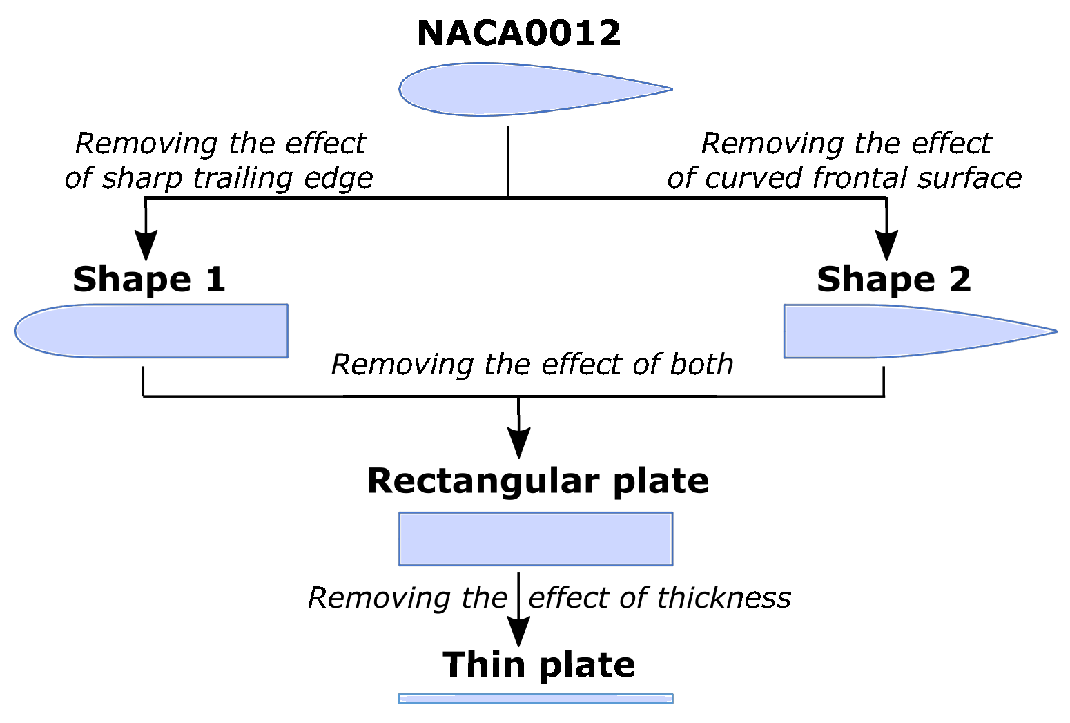
2.1. Mapping the Hydrofoil Shape

For the study on the role of curvature, specifically the front and rear shape, and thickness of the hydrofoil, Figure 1 depicts various shapes that are considered in the present study. The different shapes are chosen in such a way that they connect the two extreme shapes (a NACA0012 airfoil and a thin flat plate) by considering the importance of the front and rear geometry, and thickness. Here, shape 1 corresponds to a NACA0012 hydrofoil with a bluff trailing edge; shape 2 corresponds to a NACA0012 hydrofoil with a bluff leading edge; the rectangular plate (effectively) corresponds to a NACA0012 hydrofoil with bluff leading as well as trailing edges; and the thin plate (effectively) corresponds to a NACA0012 hydrofoil or a rectangular plate with negligible thickness. Thus, comparing the NACA0012 hydrofoil with shape 1 explores the role of a tapering tail, a NACA0012 hydrofoil with shape 2 helps us understand the role of a rounded leading edge, a NACA0012 hydrofoil transformed into a rectangular plate helps to understand the combined role of a rounded edge and tapered tail, and finally a NACA0012 airfoil transformed into a thin plate investigates the role of thickness on the propulsive performance.

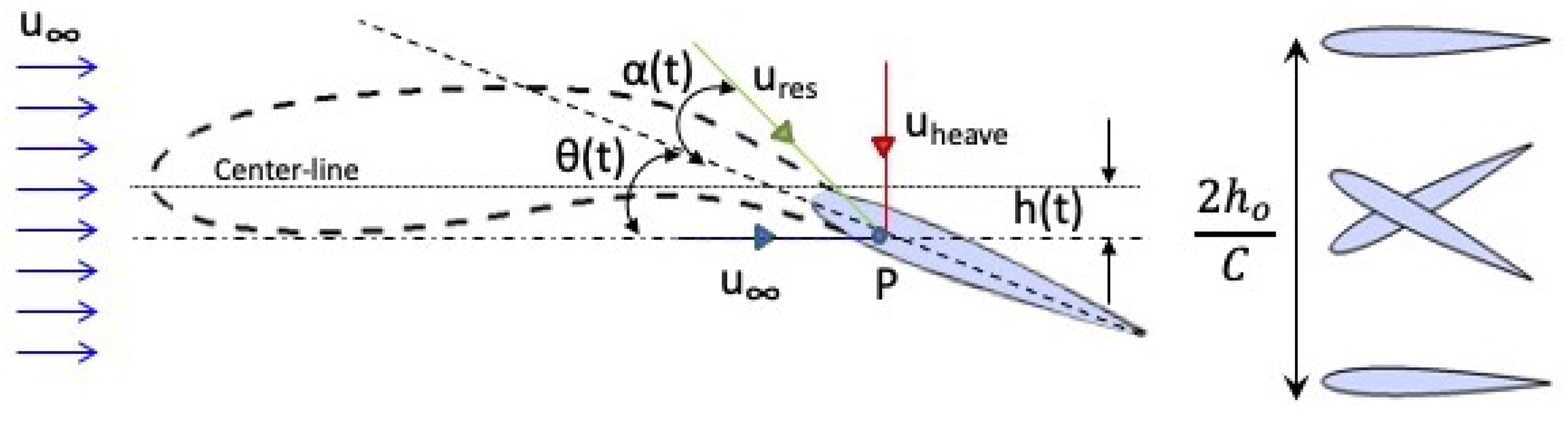
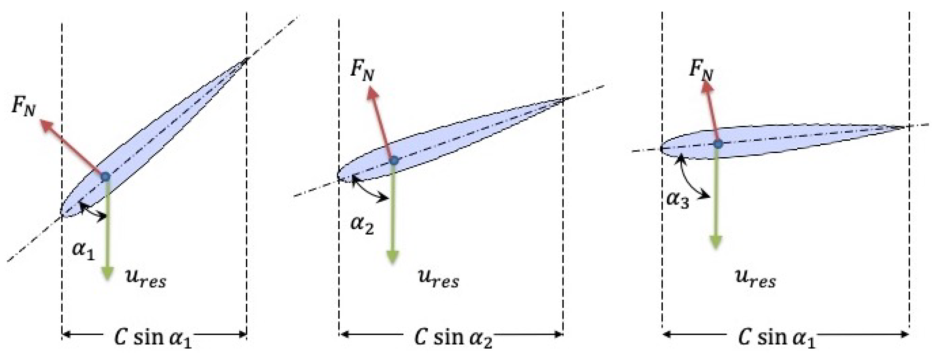
2.2. Oscillation Kinematics and Other Parameters of Interest

The oscillatory motion of the caudal (i.e., rear) fin of a fish can be modeled as a coupled pitching and heaving symmetric hydrofoil with a high aspect ratio [11,27]. This high aspect ratio allows the derivation of the three-dimensional flow characteristics around the foil from the two-dimensional flow considerations [12]. Figure 2 shows the schematic figure of a carangiform/thunniform fish about the medio-frontal plane. The hatched region shows the modeled caudal fin performing coupled pitching-and-heaving motions about the pivot point P in a freestream flow of velocity $u_{\infty }$. The corresponding motion can be replicated by sinusoidal motion for both the heave and pitch [13], given as

$$\begin{array}{c}\hfill h\left(t\right)=h_{0}sin\left(2\pi ft\right),\\ \hfill \theta \left(t\right)={\theta }_{0}sin(2\pi ft+\varphi ),\end{array}$$

(1)

where $h_0$ is the maximum heave amplitude, f is the frequency, ${\theta }_0$ is the maximum pitching amplitude, and $\varphi$ is the phase-angle difference between heave and pitch. Notice from the figure that due to heaving motions, the hydrofoil moves at an additional velocity, the heave velocity $u_{heave}=dh/dt$, which results in a change in the resultant velocity $\left(u_{res}\right)$ of the foil. Thus, the instantaneous angle of attack $\alpha \left(t\right)$ is no longer equal to pitching angle $\theta \left(t\right)$ [12] and can be given as:

$$\begin{array}{c}\hfill \tan \left[\alpha \left(t\right)+\theta \left(t\right)\right]=\frac{1}{u_{\infty }}\frac{dh\left(t\right)}{dt},\\ \hfill {\alpha }_{max}=max\left[{\tan }^{-1}\left(\frac{1}{u_{\infty }}\frac{dh\left(t\right)}{dt}\right)-\theta \left(t\right)\right].\end{array}$$

(2)

For analyzing the output performance, the non-dimensional parameters considered in the study are the thrust coefficient $C_T$, lateral force coefficient $C_L$, input power coefficient $C_P$, and propulsive efficiency ${\eta }_P$, defined as, respectively,

$$C_T=\frac{F_T}{\raisebox{1ex}{$1$}\!\left/ \!\raisebox{-1ex}{$2$}\right.\rho u_{\infty }^{2}C},C_L=\frac{F_L}{\raisebox{1ex}{$1$}\!\left/ \!\raisebox{-1ex}{$2$}\right.\rho u_{\infty }^{2}C},C_P=\frac{\int c_L{V}_{body}dS}{\raisebox{1ex}{$1$}\!\left/ \!\raisebox{-1ex}{$2$}\right.\rho u_{\infty }^{3}C},$$

(3)

$${\eta }_p=\frac{P_{out}}{P_{in}}=\frac{{\overline{F}}_T{u}_{\infty }}{\overline{\int c_L{V}_{body}dS}}=\frac{{\overline{C}}_T}{{\overline{C}}_P}.$$

(4)

Here, $F_T$ and $F_L$ are the net forces acting in the streamwise and lateral direction, respectively, and are calculated from the integration of pressure and viscous forces over the hydrofoil. Further, $\rho$ is the density of the surrounding fluid, $c_L$ is the local lateral force coefficient per unit surface area of the hydrofoil, and $V_{body}$ is the lateral velocity of an oscillating hydrofoil. The propulsive efficiency ${\eta }_P$ is defined as the ratio of the net output power to the input power [28,29], where an overbar represents time-averaged values obtained by using at least twenty oscillation cycles following statistical convergence of the simulations.

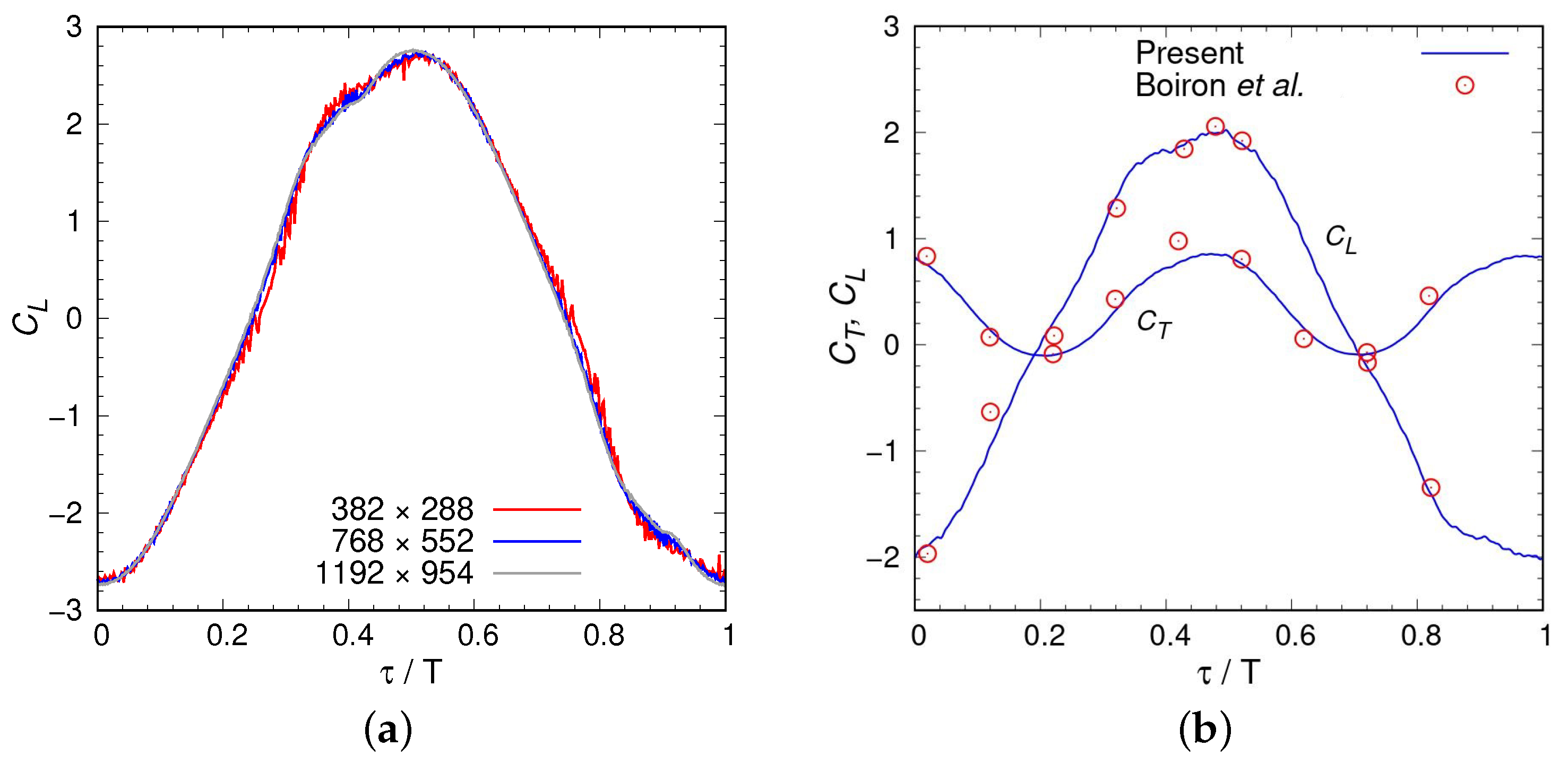
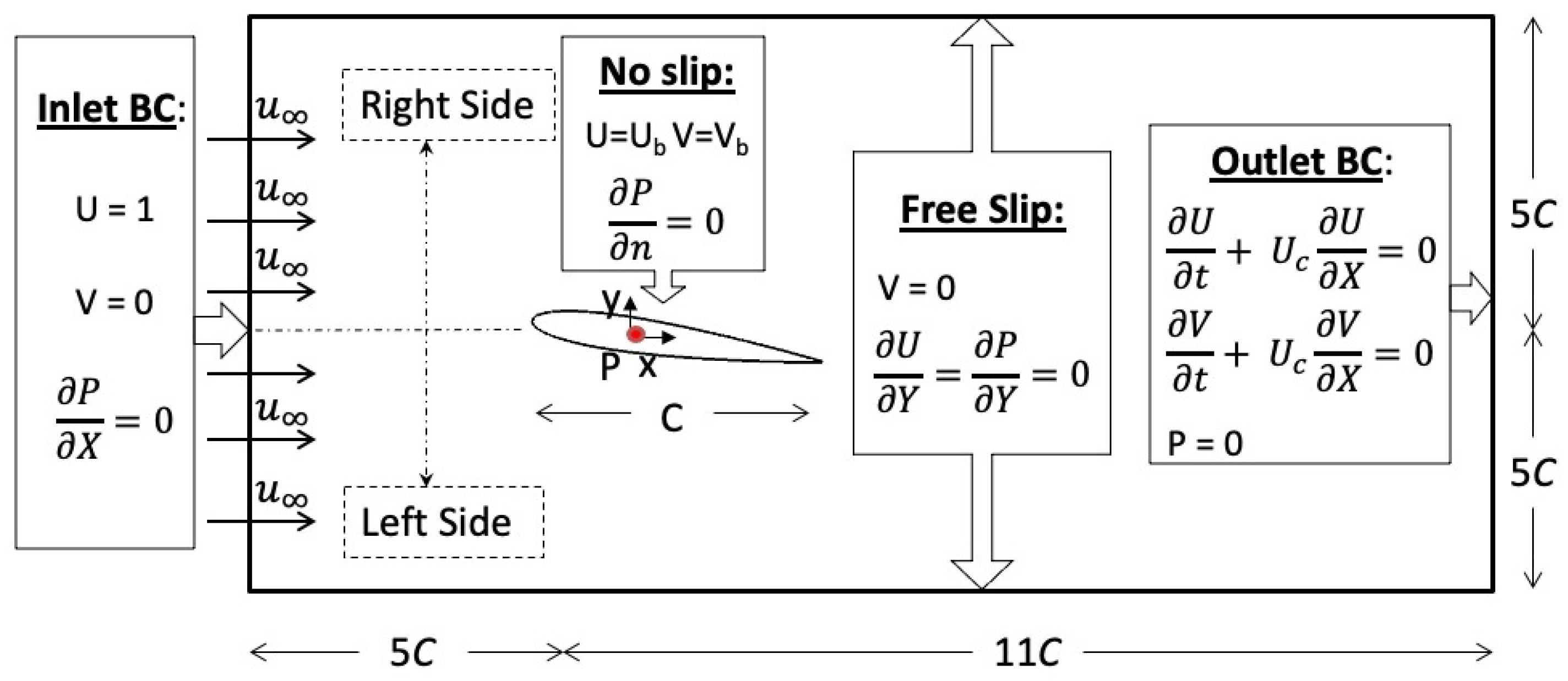
2.3. Governing Equations and Numerical Details

For an oscillating hydrofoil, Zurman et al. [30] found that the flow and forces are effectively two-dimensional for a NACA0016 hydrofoil at $St=0.15-0.45$ and $Re=5300$. Thus, for the present cases at $St=0.25$ and $Re=5000$, 2D numerical simulations are performed using an in-house code based on a level-set function-based immersed interface method (LS-IIM). The LS-IIM-based code was developed in the CFD lab at IIT Bombay by Thekkethil [31], in which the temporal variation in the solid–fluid interface is tracked by using a normal signed distance-based level set function, $\mathrm{\Phi }$. At each time step, the value of $\mathrm{\Phi }$ is calculated using the minimum distance and winding algorithms, governed by the predefined kinematics of oscillation (discussed in Section 2.2). The positive $\mathrm{\Phi }$ values represent fluid cells, whereas negative values represent solid cells. The fluid dynamics of the present problem are governed by the incompressible Navier–Stokes equation. In non-dimensional form, these are given by

$$\mathrm{Continuity}:\nabla ·\overrightarrow{U}=0,$$

(5)

$$\mathrm{Momentum}:\frac{\partial \overrightarrow{U}}{\partial \tau }+\nabla ·\left(\overrightarrow{U}\overrightarrow{U}\right)=-\nabla P+\frac{1}{Re}{\nabla }^2\overrightarrow{U},$$

(6)

where $\overrightarrow{U}$$(\equiv \overrightarrow{u}/u_{\infty },u_{\infty }$ is the freestream velocity) is the non-dimensional velocity vector and P ($\equiv p/(\rho u_{\infty }^2$), $\rho$ is the density of the surrounding fluid) is the non-dimensional pressure.

The LS-IIM uses the finite-volume method to discretize the above equations in space. Further, it is based on a fully implicit pressure projection method on a collocated grid. The non-linear advection term of the Navier–Stokes equation is integrated using the QUICK (Quadratic Upstream Interpolation for Convective Kinematics) scheme, while the CDS (Central Difference Scheme) is used for the diffusion term. More details of LS-IIM can be found in Thekkethil and Sharma [1].

2.4. Computational Details

Figure 3 shows the non-dimensionalized computational domain and the boundary conditions for the present problem on flow past an oscillating hydrofoil. The chord length C and the freestream velocity $u_{\infty }$ are taken as the length and the velocity scale for the problem. The x-direction is aligned with the streamwise direction, while the y-direction is aligned with the lateral direction of the flow. The domain measures $16C$ in the streamwise direction, with the leading edge of the hydrofoil placed $5C$ from the inlet. The lateral dimension of the domain is $10C$, with the hydrofoil located at the center. This provides a maximum lateral blockage $(0.12C/10C)$ of 1.2%, ensuring a minimal effect of the lateral boundaries on the hydrodynamics of oscillation.

In Figure 3, U and V correspond to the non-dimensional velocities in the streamwise and lateral direction, respectively. The boundary condition at the inlet corresponds to a constant velocity (equal to the freestream velocity, $u_{\infty }$). A convective boundary condition, with a convective velocity $U_c$ equal to one, has been used at the outlet. A free-slip or symmetry boundary condition is used for the lateral boundaries. The hydrofoil is assumed to be non-deforming, and a no-slip (for the velocity) and a Neumann boundary condition (for pressure) have been employed at its surface.

For the grid independence study, we considered three non-homogeneous structured grids of sizes: $382\times 288$, $768\times 552$, and $1192\times 954$. For each grid, a uniform size fine cell of size $\Delta x=\Delta y=0.01,0.05$, and 0.0025 is used in the region closer to the hydrofoil, and a uniform coarse cell size of $\Delta x=\Delta y=0.5,0.25$ and 0.125 is used in the far field. The finest and coarsest grid zones are connected using a hyperbolic stretching function, with a maximum expansion ratio of less than 1.01. For ${\alpha }_{max}={30}^{\circ }$, $h_{\circ }/C=0.75$, $St=0.25$, and $Re=5000$, Figure 4a shows no significant visual difference in the temporal variation in the lateral force coefficient $C_L$ between the two finest grids. Therefore, all further simulations for the present problem are carried out using the intermediate $768\times 552$ grid size, noting that it has 200 points across the hydrofoil chord. The simulations are carried out in series on the local system with 32 GB RAM for a total of 48 simulation hours per case.

The numerical method used for the present study has already been applied successfully to various similar fluid–structure interaction (FSI) problems [1,32,33,34,35,36,37]. However, a further validation study has been carried out by comparing our results with that documented by Boiron et al. [38] and is presented in Figure 4b. The figure shows an excellent agreement between the present and published results for the temporal variation in the thrust and lift coefficients at ${\alpha }_{max}={20}^{\circ }$, $h_{\circ }/C=0.75$, $St=0.3$ and $Re=4000$. The percentage of difference is within 2% and 5% for the lift and thrust coefficients, respectively.

Figure 4. Validation of the computer code for an oscillating NACA0012 hydrofoil. (a) Grid independence study. Temporal variation of the lift coefficient $C_L$ at ${\alpha }_{max}={30}^{\circ }, h_{\circ }/C=0.75, St=0.25$ and $Re=5000$. (b) Code verification study comparing predictions against those of Boiron et al. [38]. Temporal variation in thrust coefficient $C_T$ and lift coefficient $C_L$ at ${\alpha }_{max}={20}^{\circ },$$h_{\circ }/C=0.75, St=0.3$ and $Re=4000$. The intermediate size grid, $768\times 552$, is used.

Figure 4. Validation of the computer code for an oscillating NACA0012 hydrofoil. (a) Grid independence study. Temporal variation of the lift coefficient $C_L$ at ${\alpha }_{max}={30}^{\circ }, h_{\circ }/C=0.75, St=0.25$ and $Re=5000$. (b) Code verification study comparing predictions against those of Boiron et al. [38]. Temporal variation in thrust coefficient $C_T$ and lift coefficient $C_L$ at ${\alpha }_{max}={20}^{\circ },$$h_{\circ }/C=0.75, St=0.3$ and $Re=4000$. The intermediate size grid, $768\times 552$, is used.

3. Results

The results section is divided into three subsections. Section 3.1 discusses the effect of varying the maximum angle of attack, ${\alpha }_{max}$, on the propulsive performance of different shaped hydrofoils. Section 3.2 discusses the correlation between the time-averaged engineering parameters and instantaneous flow parameters using a cause-and-effect-based study and instantaneous vorticity in the vicinity of the hydrofoils at the extreme rightward lateral position. Section 3.3 examines hydrofoil cases at maximum efficiency to study the role of the phase difference $\varphi$ between heave and pitch. In both Section 3.1 and Section 3.3, the time-averaged performance parameters are calculated over twenty oscillation cycles following the statistical convergence of the simulations.

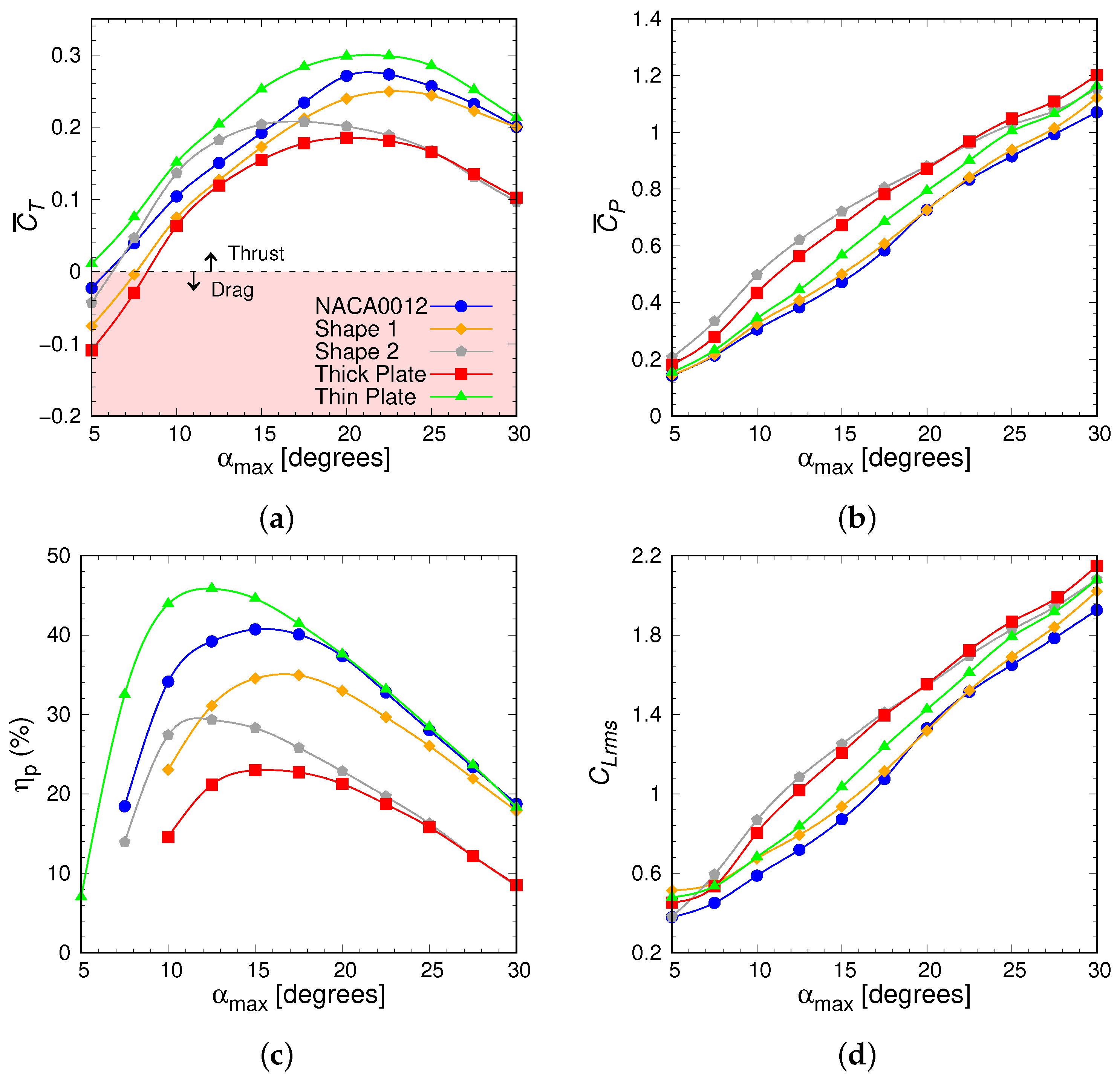
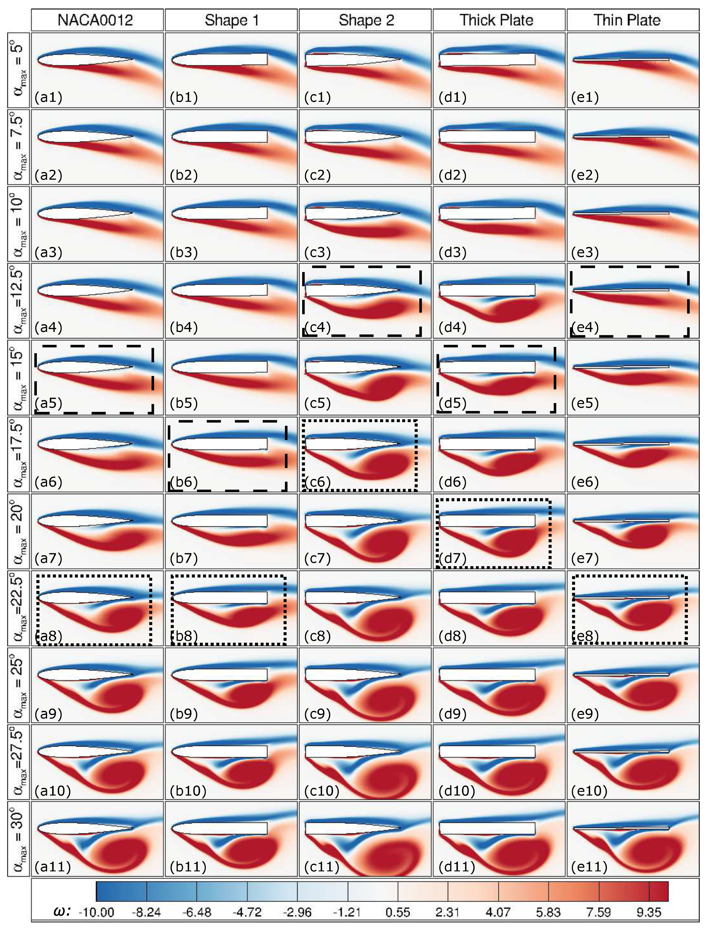
3.1. Effect of Curvature Variations on Hydrodynamic Performance

Considering the five different shapes of the hydrofoil (Figure 1), Figure 5 presents the effect of curvature and thickness on the time-averaged propulsive performance of a hydrofoil for various angles of attack, ${\alpha }_{max}=5^{\circ }-{30}^{\circ }$, at $St=0.25$, $h_0/C=0.75$, $\varphi ={90}^{\circ }$ and $Re=5000$. This leads to the pitching amplitude ${\theta }_0\sim {34}^{\circ }-8^{\circ }$ (Equation (1)).

For the mean thrust coefficient ${\overline{C}}_T$, Figure 5a shows that the magnitudes of ${\overline{C}}_T$ for the NACA0012 and those with a bluff leading/trailing edge (shape 1 and shape 2) are bounded within the magnitude of ${\overline{C}}_T$ for the thin plate and thick plate. With an increase in ${\alpha }_{max}$, the figure shows an increasing–decreasing trend for ${\overline{C}}_T$ with its maximum close to ${\alpha }_{max}=22.5^{\circ }$ for the different shapes; the exception is shape 2, which achieves its maximum ${\overline{C}}_T$ at ${\alpha }_{max}=17.5^{\circ }$. Further, at lower values of ${\alpha }_{max}$, ${\overline{C}}_T$ for bluff frontal edge-based shape 2 approaches that of a thin plate, while ${\overline{C}}_T$ for bluff trailing edge-based shape 1 approaches that of a thick plate. However, at higher values of ${\alpha }_{max}$, the reverse applies; that is, ${\overline{C}}_T$ for shape 1 approaches ${\overline{C}}_T$ of a thin plate, while ${\overline{C}}_T$ for shape 2 approaches that of a thick plate. The figure also shows the drag-to-thrust transition for different shapes with increasing ${\alpha }_{max}$, except for the thin plate with a net thrust even at a very low ${\alpha }_{max}=5^{\circ }$. For other hydrofoils, the figure shows that the transition occurs first for hydrofoils with a tapered trailing edge (NACA0012 and shape 2), compared with hydrofoils with a bluff trailing edge (shape 1 and the thick plate).

For the mean input power coefficient ${\overline{C}}_P$, Figure 5b shows an apparent increasing ${\overline{C}}_P$ with increasing ${\alpha }_{max}$, with ${\overline{C}}_P$ for the different shapes bounded within the maximum ${\overline{C}}_P$ for shape 2 and minimum ${\overline{C}}_P$ for the NACA0012 airfoil. Further, the figure shows that ${\overline{C}}_P$ is smaller for shapes with a rounded frontal edge (NACA0012 airfoil, shape 1) compared with bluff frontal edges (the flat plate, shape 2 and the thick plate), and the trend is independent of ${\alpha }_{max}$ for the hydrofoil. Moreover, for the bluff frontal-edge hydrofoils, ${\overline{C}}_P$ increases with frontal surface area, i.e., ${\overline{C}}_P$ is larger for shape 2 and the thick plate compared to that for the thin plate at any ${\alpha }_{max}$.

Similar to the variation with ${\overline{C}}_T$, Figure 5c shows that ${\eta }_P$ for the different shapes is again bounded between the values for the thin and thick plate for any ${\alpha }_{max}$. Note that the efficiency curve contains only those cases that resulted in a net mean thrust. Furthermore, the figure shows that the nature of the ${\eta }_P$ curve is also of increasing–decreasing type. However, for three of the foil shapes, the maximum ${\eta }_P$ occurs at ${\alpha }_{max}={15}^{\circ }$–$17.5^{\circ }$; this is not the case for the thin plate and shape 2, which have maximum ${\eta }_P$ at ${\alpha }_{max}=12.5^{\circ }$. At larger angles of attack, ${\alpha }_{max}\ge 20.0^{\circ }$, the figure shows that ${\eta }_P$ for the NACA0012 matches that of a thin plate, whereas the ${\eta }_P$ for shape 2 matches that of a thick plate. Further, by comparing shape 1 with the NACA0012 airfoil and shape 2 with the thick plate, it can be seen that ${\eta }_P$ is greater for shapes that possess a tapered end. However, the benefits of possessing a tapered end decrease with increasing ${\alpha }_{max}$.

For the rms variation in the lift coefficient, $C_{L,\mathrm{rms}}$, Figure 5d shows that the variation is similar to the variation in ${\overline{C}}_P$ with ${\alpha }_{max}$, as discussed above. For instance, the magnitude of $C_{L,\mathrm{rms}}$ increases with ${\alpha }_{max}$; for any ${\alpha }_{max}$, the magnitude of $C_{L,\mathrm{rms}}$ for different shapes is bounded within the maximum $C_{L,\mathrm{rms}}$ for shape 2 and the minimum $C_{L,\mathrm{rms}}$ for the NACA0012 airfoil, showing that shape 2 is the least stable and the NACA0012 airfoil is the most stable hydrofoil for propulsion. Further, it is important to notice that the $C_{L,\mathrm{rms}}$ of shapes with a rounded frontal shape is smaller compared to shapes with a bluff frontal surface, which leads to a more stable propulsion for shapes with a rounded frontal area.

The above-discussed increasing–decreasing trend for ${\overline{C}}_T$ and the increasing trends for ${\overline{C}}_P$ and $C_{L,\mathrm{rms}}$ with increasing ${\alpha }_{max}$ are at least partially understandable as these parameters are directly proportional to the surrounding fluid displaced by the hydrofoil. Thus, these parameters are directly proportional to the projected lateral surface area ($Csin\left(\alpha \right)$) of the hydrofoil. To discuss this, Figure 6 shows instantaneous schematics of a hydrofoil at three values of ${\alpha }_{max}$ (${\alpha }_1<{\alpha }_2<{\alpha }_3$). For simplicity, we have assumed that the hydrofoil is oscillating in a still fluid, resulting in the vertical relative velocity $u_{res}$. With increasing ${\alpha }_{max}$, the figure shows that the projected lateral surface area of the hydrofoil increases, resulting in an increased volume of displaced fluid. Thus, a larger ${\overline{C}}_P$ is required for an oscillating hydrofoil to perform its movement at a larger ${\alpha }_{max}$.

Figure 6 also shows the normal direction in which the hydrodynamic force acts from the fluid to the hydrofoil. The axial component of this force provides the instantaneous thrust force, while the lateral component provides the instantaneous lift force. It can be seen from the figure that with increasing ${\alpha }_{max}$, both the projected lateral surface area and lift component increase, resulting in an almost linear enhancement of $C_{L,\mathrm{rms}}$ with ${\alpha }_{max}$. In contrast, for $C_T$, there is a trade-off between increasing surface area and decreasing axial component, resulting in an increasing–decreasing variation. However, it is important to notice from Figure 5 that the magnitude of engineering parameters is different for different shapes. Further, the ${\alpha }_{max}$ at which maximum ${\overline{C}}_T$ and ${\eta }_p$ occur is different for different shapes. Thus, a more detailed study is needed; this is attempted in the next section (Section 3.2) by correlating the engineering parameters with the flow structures near the vicinity of the hydrofoil.

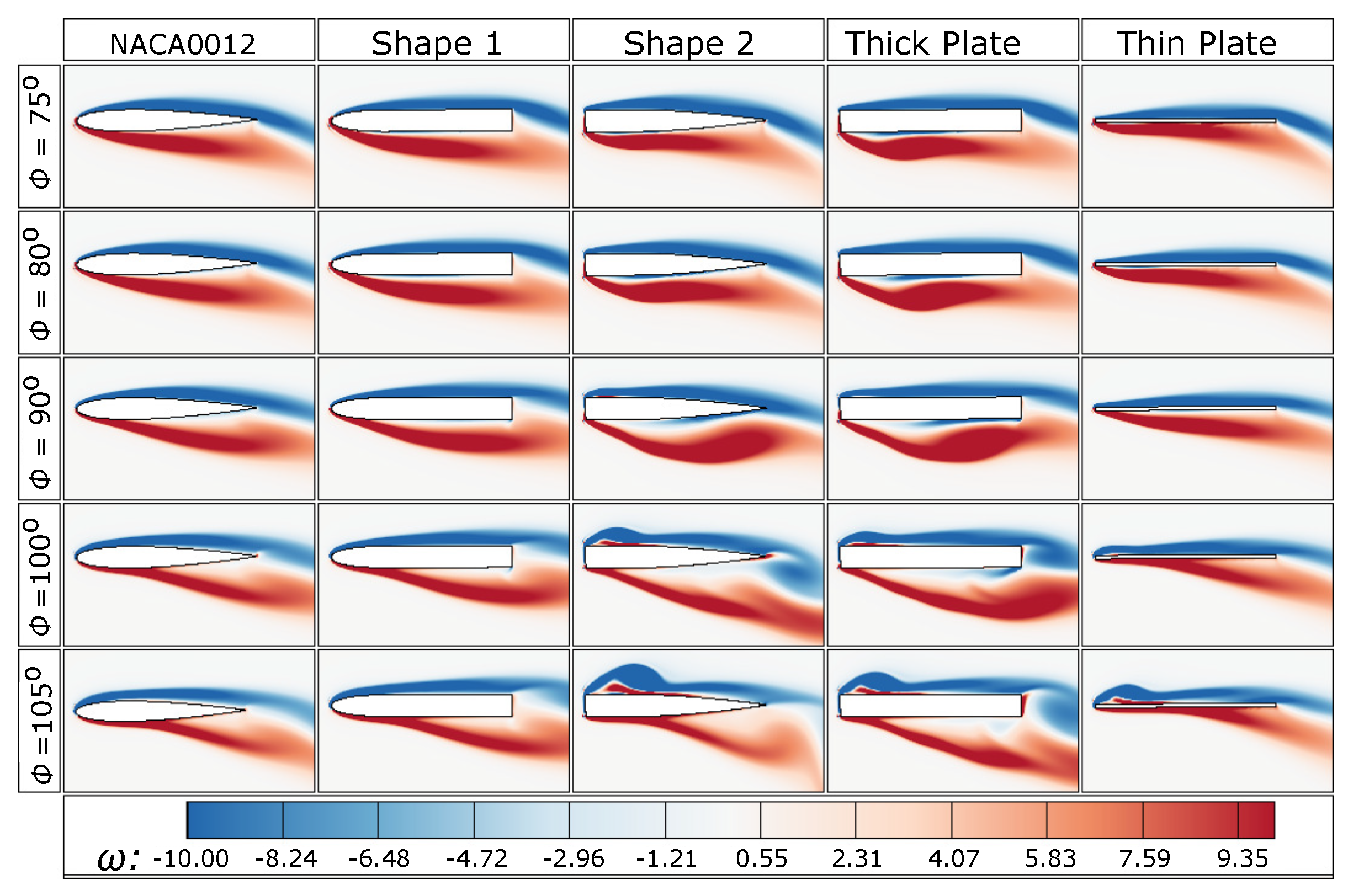
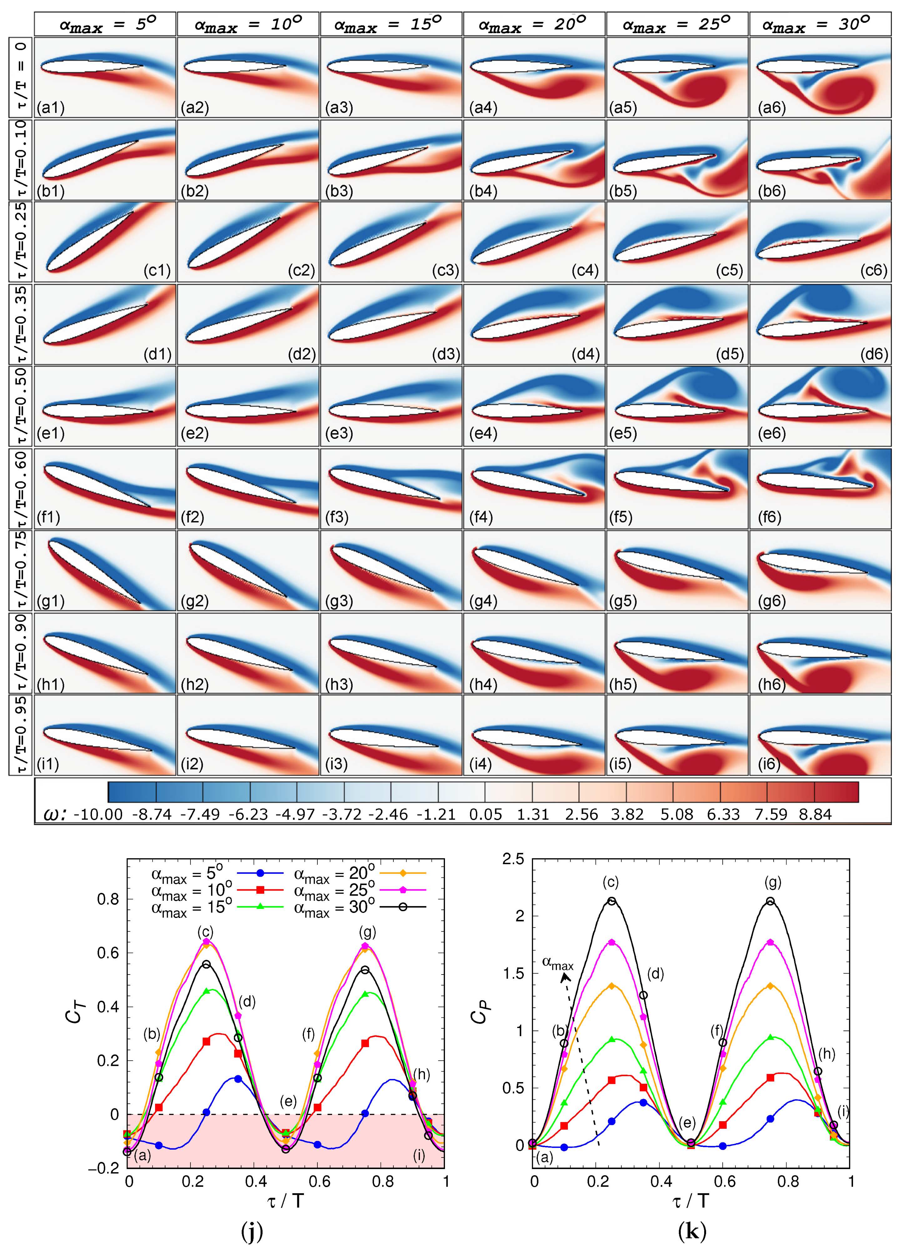
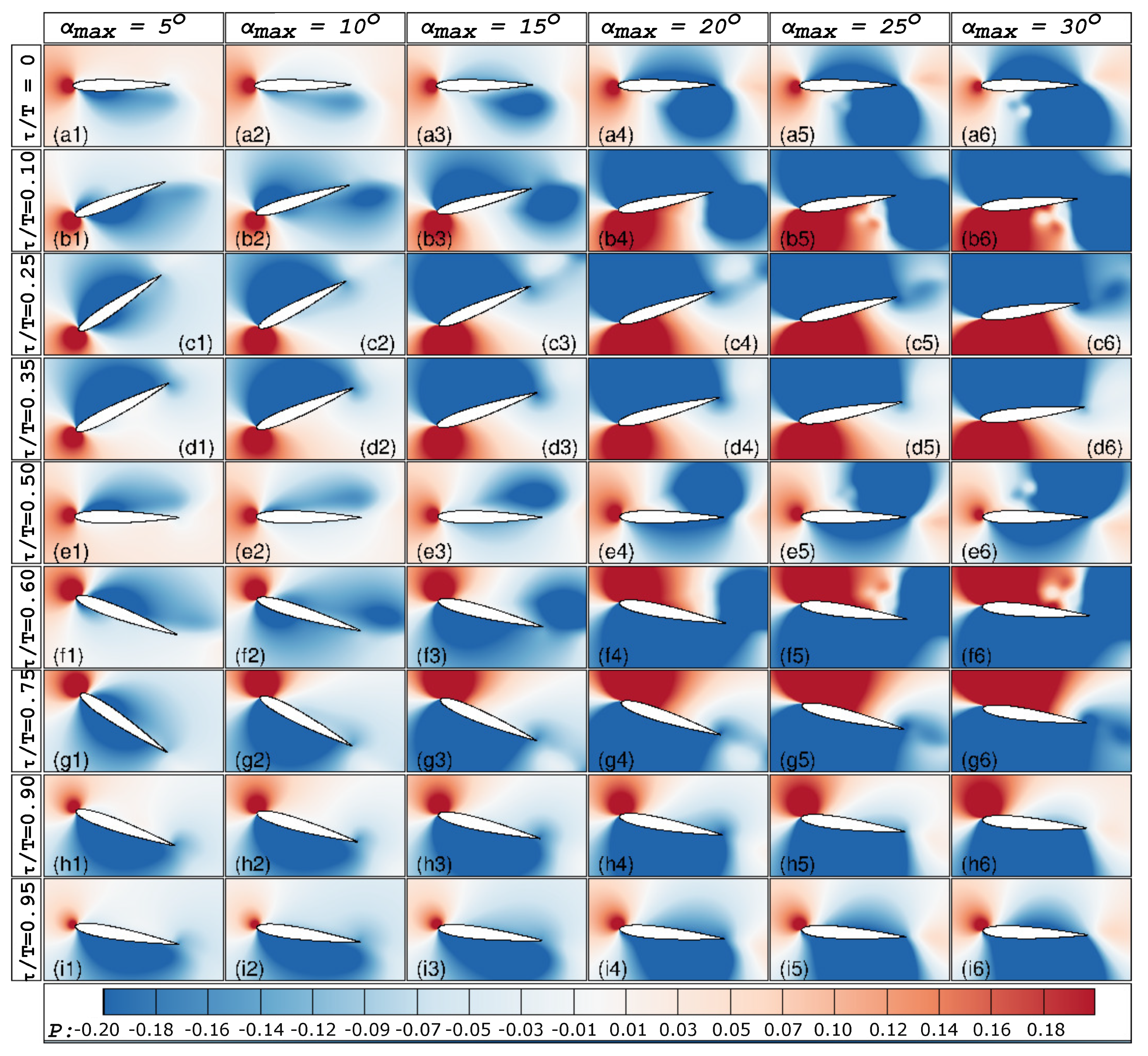
3.2. Flow Characteristics

The correlation between the above-discussed time-averaged engineering parameters with the instantaneous flow parameters is accomplished in two steps. In the first step, the instantaneous pressure contours in the vicinity of the hydrofoil are correlated with the corresponding instantaneous vortex structure and engineering parameters. For ease of understanding, the study is conducted only for an oscillating NACA0012 hydrofoil for a range of ${\alpha }_{max}$. The corresponding study is known as a unified cause-and-effect-based CFD analysis, and has been proposed by Sharma [39]. The study helps to correlate the time-averaged engineering parameters with the instantaneous vortex structure when the NACA0012 hydrofoil is at the rightmost lateral position. In the second step, the correlation developed in the first step is applied to differently shaped hydrofoils.

Over one oscillation period, Figure 7 and Figure 8 show a unified cause-and-effect-based analysis by plotting the time variation in 2D plots for flow properties and 1D line-plots for propulsive performance parameters for ${\alpha }_{max}$ in the range $5^{\circ }\le {\alpha }_{max}\le {30}^{\circ }$. The 2D contour plots Figure 7a–i and Figure 8a–i are for the vortex structure and pressure contours in the vicinity of the hydrofoil, respectively, while the 1D plots, Figure 7j,k, are for the thrust $C_T$ and power $C_P$ coefficients.

At $\tau /T=0$, Figure 7 shows the onset of the leftward movement of the hydrofoil from its extreme right lateral position. At this instant of time, a net drag acts on all the hydrofoils independent of ${\alpha }_{max}$; however, the magnitude of drag is larger for hydrofoils with a higher ${\alpha }_{max}$, as shown in Figure 7j. The reason behind this increase in drag with ${\alpha }_{max}$ can be seen in the instantaneous vortex contours of Figure 7(a1–a6). For ${\alpha }_{max}=5^{\circ }$, the figure shows a fully attached flow across the hydrofoil, while the flow separates for hydrofoils with ${\alpha }_{max}>5^{\circ }$—in this case, the flow starts to separate from the posterior region of the foil, and the point of separation moves towards the leading edge and becomes stronger with increasing ${\alpha }_{max}$. The stronger flow separation causes a stronger pressure gradient along the chord (Figure 8(a1–a6)), resulting in higher drag.

Figure 7(b1–b6) show that the hydrofoil rotates in the counter-clockwise (CCW) direction with further leftward movement. With this movement to $\tau /T=0.1$, Figure 7j shows the crossover from instantaneous drag to thrust for all ${\alpha }_{max}$, except for ${\alpha }_{max}=5^{\circ }$ for which crossover occurs later at $\tau /T=0.25$. Further, the figure shows that the magnitude of instantaneous $C_T$ at $\tau /T=0.1$ increases with increasing ${\alpha }_{max}$, reaches its maximum at ${\alpha }_{max}={20}^{\circ }$, and then decreases. In contrast, Figure 7k shows that the instantaneous power coefficient $C_P$ increases with ${\alpha }_{max}$. The corresponding vortex structure in Figure 7(b1–b6) shows that the increase in instantaneous $C_T$ and $C_P$ with ${\alpha }_{max}$ is due to an increase in the strength of flow separation. However, above ${\alpha }_{max}={20}^{\circ }$, the strength of the flow separation is too large such that it draws the flow around the trailing edge of the hydrofoil, resulting in a reduction in net instantaneous thrust. With the further leftward movement to $\tau /T=0.25$, Figure 7j,k show that the hydrofoils reach their maximum instantaneous $C_T$ and $C_P$, except for ${\alpha }_{max}=5^{\circ }$. Further, the figure shows that the largest instantaneous $C_T$ occurs for ${\alpha }_{max}={25}^{\circ }$, in contrast to $\tau /T=0.1$. The change in trend is due to the flow remaining attached up to ${\alpha }_{max}={20}^{\circ }$ (Figure 7(c1–c4)), a small separated flow at ${\alpha }_{max}={25}^{\circ }$ (Figure 7(c5)), and a larger separation for ${\alpha }_{max}={30}^{\circ }$ (Figure 7(c6)).

With further leftward movement, Figure 7(d1–d5) show that the CCW rotation of the hydrofoil switches to clockwise (CW) rotation, and the hydrofoils decelerate, reaching the extreme leftmost position. This deceleration of the hydrofoil reduces the instantaneous positive leftward pressure for all the cases, except for ${\alpha }_{max}=5^{\circ }$—compare Figure 8(c1–c5) with Figure 8(d1–d5). The reduction in pressure reduces the pressure gradient, resulting in a reduction in the instantaneous thrust and power for all cases, except for ${\alpha }_{max}=5^{\circ }$, as shown in Figure 7j,k, respectively. Further, the switch in rotation from CCW to CW enhances the flow separation from the hydrofoil’s rightward side, resulting in the continuation of the trend of increasing instantaneous $C_T$ with ${\alpha }_{max}$ up to ${\alpha }_{max}={25}^{\circ }$ and then decreasing, as observed for $\tau /T=0.25$. The retardation continues as the hydrofoil approaches the extreme leftmost position (completing half a cycle), resulting in a further decrease in instantaneous thrust and power, as shown in Figure 7j,k.

For the subsequent half cycle, where the hydrofoil moves from the extreme leftmost to the rightmost position, Figure 7 and Figure 8 show an opposite nature of periodic variation in vortex structures and pressure on the two sides of the foil, resulting in similar instantaneous thrust and power curve.

Therefore, by correlating the instantaneous vortex structure with the thrust and power coefficients for a cycle of oscillation of the NACA0012 hydrofoil at different ${\alpha }_{max}$, it can be concluded that any amount of flow separation enhances the power consumed by the hydrofoil for performing its oscillation motion. In contrast, a moderately strong degree of flow separation (until it becomes so strong that it starts pulling a significant amount of fluid around the trailing edge) enhances the thrust. For further investigation, Figure 9 compares the instantaneous vortex structure in the vicinity of different shaped hydrofoils at their extreme rightward lateral position for various ${\alpha }_{max}$. It can be seen from the highlighted rectangular regions in the figure that the ${\eta }_{max}$ for any shape occurs at that ${\alpha }_{max}$, for which there is a small degree of flow separation with almost no roll-up into a separating vortex. On the other hand, the highlighted cases for ${\overline{C}}_{T,max}$ are those at which moderately strong flow separation occurs with no induction of a significant amount of fluid transferring around the trailing edge.

Figure 9 also shows the effect of ${\alpha }_{max}$ and geometrical parameters on the flow separation. For any shape, an increasing ${\alpha }_{max}$ increases the magnitude of flow separation and brings the point of separation close to the leading edge. Geometrical features such as a bluff leading edge, tapered tail, and high thickness enhance the flow separation, while those such as a rounded leading edge and a flattened tail reduce the magnitude of flow separation.

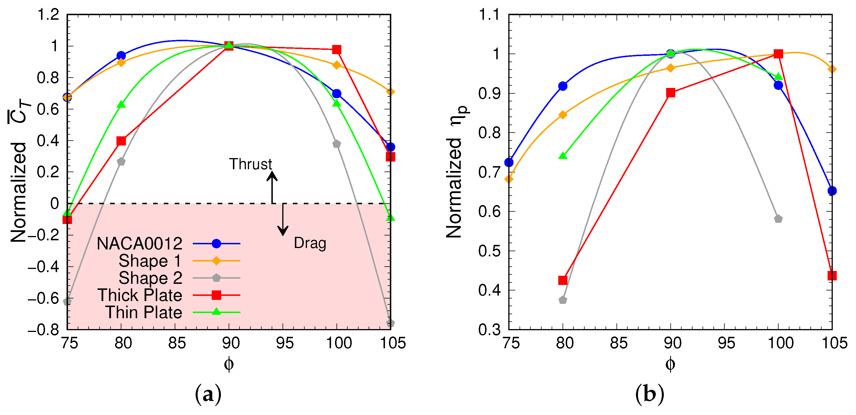
3.3. Effect of Phase Difference between Heave and Pitch $\varphi$ on Hydrodynamic Performance

In this section, the effect of the phase difference between heave and pitch, $\varphi$, on the propulsive performance of the hydrofoils is presented for cases at ${\eta }_{p,max}$, as observed in Section 3.1. This corresponds to ${\alpha }_{max}={15}^{\circ }$ for the NACA0012 airfoil and thick plate, ${\alpha }_{max}=17.5^{\circ }$ for shape 1, and ${\alpha }_{max}=12.5^{\circ }$ for shape 2 and the thin plate for phase differences $\varphi ={75}^{\circ }-{105}^{\circ }$, all at constant $St=0.25$, $h_o/C=0.75$ and $Re=5000$.

Figure 10 shows the variation in the normalized ${\overline{C}}_T$ and ${\eta }_p$ with phase difference $\varphi$ for different shaped hydrofoils at ${\eta }_{p,max}$, i.e., ${\alpha }_{max}={15}^{\circ }$ for the NACA0012 airfoil and thick plate, ${\alpha }_{max}=17.5^{\circ }$ for shape 1, and ${\alpha }_{max}=12.5^{\circ }$ for shape 2 and the thin plate. Here, the normalized values are obtained by normalizing with corresponding values at $\varphi ={90}^{\circ }$. For all cases, the figure shows that both the maximum thrust and efficiency occur in a narrow range of phase difference ${90}^{\circ }\le \varphi \le {100}^{\circ }$; this indicates that the optimal phase difference for propulsion is independent of the shape and shows the hydrodynamic (and evolutionary) reason behind its adoption by different body–caudal fin (BCF) fish in nature.

The occurrence of maximum efficiency and thrust coefficient at phase angles ${90}^{\circ }\le \varphi \le {100}^{\circ }$ is explained here using the analogy developed in Section 3.1 between the instantaneous wake structure in the vicinity of hydrofoil (at maximum heave position) and the engineering parameters. Similar to Figure 9, Figure 11 also shows that the maximum efficiency occurs at those $\varphi$ for which there is a small degree of flow separation with no roll-up of a separating vortex. Similarly, the maximum ${\overline{C}}_{T,max}$ occurs at those $\varphi$ for which moderately strong flow separation occurs with no significant induction of fluid around the trailing edge.

Figure 11 also shows the effect of the phase difference $\varphi$ and geometrical parameters on the instantaneous vorticity in the vicinity of the hydrofoils. It is seen that the flow separation for all the shapes reduces by decreasing the phase difference below $\varphi ={90}^{\circ }$. However, the flow separation enhances, and the point of separation travels posterior (towards the tail) by increasing the phase difference above $\varphi ={90}^{\circ }$. Further, by increasing the phase difference above $\varphi ={90}^{\circ }$, secondary flow separation occurs from the rightward leading edge for shapes with a bluff leading edge (shape 2, the thick plate and the thin plate).

4. Conclusions

The present study documents and contributes towards understanding the role of an oscillating hydrofoil’s curvature/shape at the leading and trailing edges, along with its thickness, in the propulsive performance at various maximum angles of attack in the range ${\alpha }_{max}=5^{\circ }-{30}^{\circ }$, and for phase differences between heave and pitch of $\varphi ={75}^{\circ }-{105}^{\circ }$, at constant $St=0.25$, $h_o/C=0.75$, and $Re=5000$. The conclusions drawn are as follows.

In terms of the role of leading- and trailing-edge curvatures, a tapered tail provides (compare NACA0012 with shape 1) a more significant thrust, consumes slightly lower power, and generates a lower $C_{L,\mathrm{rms}}$. On the other hand, a rounded leading edge (compare the NACA0012 airfoil with shape 2) provides a smaller and larger thrust for ${\alpha }_{max}<{15}^{\circ }$ and ${\alpha }_{max}>{15}^{\circ }$, respectively. However, the power consumption and $C_{L,\mathrm{rms}}$ reduce significantly. Thus, these leading and trailing curvatures enhance the oscillating hydrofoil’s overall propulsive performance and stability. Therefore, it is evident that the combination of the rounded leading edge and tapered tail (compare the NACA0012 airfoil and thick plate) provides better thrust and lower power consumption and $C_{L,\mathrm{rms}}$, providing overall enhanced propulsion. For the role of hydrofoil thickness (compare the thick and thin plates), a greater thickness reduces the net thrust and enhances the power consumption and $C_{L,\mathrm{rms}}$, resulting in degradation of the overall propulsive performance and stability of an oscillating hydrofoil. Finally, for the role of the phase difference between heave and pitch, it was found that both the maximum thrust and efficiency occur over a narrow range ${90}^{\circ }\le \varphi \le {100}^{\circ }$ independent of the hydrofoil geometry.

The hydrodynamic reason behind the above variation is explained by correlating both the time-varying and time-instantaneous vortex structures in the vicinity of the hydrofoil with the corresponding engineering parameters. It is found that any amount of flow separation enhances the power consumed by the hydrofoil for performing its oscillation motion. In contrast, a moderate flow separation enhances the thrust generated. For all the different-shaped hydrofoils examined, the maximum efficiency occurs at those ${\alpha }_{max}$ at which there is a small degree of flow separation with no roll-up of separating vortex. In comparison, maximum thrust generation occurs when there is a moderately strong flow separation with no induction of a significant quantity of fluid around the trailing edge. For any ${\alpha }_{max}$, flow separation can be controlled by the geometrical parameters of the hydrofoil. A rounded leading edge and flattened tail reduce the magnitude of flow separation, while a bluff leading edge, tapered tail, and increased thickness enhance it.

We anticipate that by contributing to an understanding of the correlation between different hydrofoil geometrical parameters with engineering parameters and flow separation, our results can aid in designing and developing more efficient modern autonomous underwater and micro air vehicles. Our results also have implications for understanding fish swimming. A fish possesses a symmetrical caudal fin with a somewhat rounded leading edge and tapered tail, and maintains a phase difference of ${90}^{\circ }$ while swimming. The results from the present study show that their NACA-like caudal fin generates high thrust, as high as that for a very thin plate, with minimum power requirement, resulting in higher propulsive efficiency. Moreover, their propulsion is very stable. A greater thickness without losing propulsive performance can give them a caudal fin with more structural strength, which is essential for directing water around it. The present study also shows that a phase difference of ${90}^{\circ }$ for any shape provides high thrust with high efficiency and stability of oscillation. Thus, an oscillating caudal fin of NACA-like shape with a ${90}^{\circ }$ phase difference between heave and pitch provides fish with an ideal combination for achieving high thrust, efficiency, and stability for propulsion.

In the current preliminary investigation, we have compared the hydrodynamics of hydrofoils with smooth, rounded leading edges and tapered tails to those with sharp leading and trailing edges. In the future, we plan to conduct a more comprehensive comparison using a non-dimensional geometric parameter that can assess the roundness and tapering of any hydrofoil shape to develop a flow law for optimization of thrust and propulsive efficiency.

References

1. Thekkethil, N.; Sharma, A. Level set function–based immersed interface method and benchmark solutions for fluid flexible-structure interaction. Int. J. Numer. Methods Fluids 2019, 91, 134–157. [Google Scholar] [CrossRef]
2. Smits, A.J. Undulatory and oscillatory swimming. J. Fluid Mech. 2019, 874, 1. [Google Scholar] [CrossRef]
3. Zdunich, P.; Bilyk, D.; MacMaster, M.; Loewen, D.; DeLaurier, J.; Kornbluh, R.; Low, T.; Stanford, S.; Holeman, D. Development and testing of the mentor flapping-wing micro air vehicle. J. Aircr. 2007, 44, 1701–1711. [Google Scholar] [CrossRef]
4. Techet, A.H. Propulsive performance of biologically inspired flapping foils at high Reynolds numbers. J. Exp. Biol. 2008, 211, 274–279. [Google Scholar] [CrossRef] [PubMed]
5. Du, R.; Li, Z.; Youcef-Toumi, K.; y Alvarado, P.V. Robot Fish: Bio-Inspired Fishlike Underwater Robots; Springer: Berlin/Heidelberg, Germany, 2015. [Google Scholar]
6. Kinsey, T.; Dumas, G. Parametric study of an oscillating airfoil in a power-extraction regime. AIAA J. 2008, 46, 1318–1330. [Google Scholar] [CrossRef]
7. Kinsey, T.; Dumas, G.; Lalande, G.; Ruel, J.; Mehut, A.; Viarouge, P.; Lemay, J.; Jean, Y. Prototype testing of a hydrokinetic turbine based on oscillating hydrofoils. Renew. Energy 2011, 36, 1710–1718. [Google Scholar] [CrossRef]
8. Zhu, Q. Optimal frequency for flow energy harvesting of a flapping foil. J. Fluid Mech. 2011, 675, 495–517. [Google Scholar] [CrossRef]
9. Wang, Z.; Du, L.; Zhao, J.; Thompson, M.; Sun, X. Flow-induced vibrations of a pitching and plunging airfoil. J. Fluid Mech. 2020, 885, A36. [Google Scholar] [CrossRef]
10. Triantafyllou, M.; Triantafyllou, G.; Gopalkrishnan, R. Wake mechanics for thrust generation in oscillating foils. Phys. Fluids A Fluid Dyn. 1991, 3, 2835–2837. [Google Scholar] [CrossRef]
11. Triantafyllou, G.S.; Triantafyllou, M.; Grosenbaugh, M. Optimal thrust development in oscillating foils with application to fish propulsion. J. Fluids Struct. 1993, 7, 205–224. [Google Scholar] [CrossRef]
12. Anderson, J.; Streitlien, K.; Barrett, D.; Triantafyllou, M. Oscillating foils of high propulsive efficiency. J. Fluid Mech. 1998, 360, 41–72. [Google Scholar] [CrossRef]
13. Read, D.A.; Hover, F.; Triantafyllou, M. Forces on oscillating foils for propulsion and maneuvering. J. Fluids Struct. 2003, 17, 163–183. [Google Scholar] [CrossRef]
14. Hover, F.; Haugsdal, Ø.; Triantafyllou, M. Effect of angle of attack profiles in flapping foil propulsion. J. Fluids Struct. 2004, 19, 37–47. [Google Scholar] [CrossRef]
15. Van Buren, T.; Floryan, D.; Smits, A.J. Scaling and performance of simultaneously heaving and pitching foils. AIAA J. 2019, 57, 3666–3677. [Google Scholar] [CrossRef]
16. Isogai, K.; Shinmoto, Y.; Watanabe, Y. Effects of dynamic stall on propulsive efficiency and thrust of flapping airfoil. AIAA J. 1999, 37, 1145–1151. [Google Scholar] [CrossRef]
17. Ramamurti, R.; Sandberg, W. Simulation of flow about flapping airfoils using finite element incompressible flow solver. AIAA J. 2001, 39, 253–260. [Google Scholar] [CrossRef]
18. Soueid, H.; Guglielmini, L.; Airiau, C.; Bottaro, A. Optimization of the motion of a flapping airfoil using sensitivity functions. Comput. Fluids 2009, 38, 861–874. [Google Scholar] [CrossRef]
19. Tuncer, I.H.; Platzer, M.F. Computational study of flapping airfoil aerodynamics. J. Aircr. 2000, 37, 514–520. [Google Scholar] [CrossRef]
20. Tuncer, I.H.; Kaya, M. Optimization of flapping airfoils for maximum thrust and propulsive efficiency. AIAA J. 2005, 43, 2329–2336. [Google Scholar] [CrossRef]
21. Young, J.; Lai, J.C. Mechanisms influencing the efficiency of oscillating airfoil propulsion. AIAA J. 2007, 45, 1695–1702. [Google Scholar] [CrossRef]
22. Guglielmini, L.; Blondeaux, P. Propulsive efficiency of oscillating foils. Eur. J. Mech. B/Fluids 2004, 23, 255–278. [Google Scholar] [CrossRef]
23. Bose, C.; Sarkar, S. Investigating chaotic wake dynamics past a flapping airfoil and the role of vortex interactions behind the chaotic transition. Phys. Fluids 2018, 30, 047101. [Google Scholar] [CrossRef]
24. Zhang, X.; Ni, S.; Wang, S.; He, G. Effects of geometric shape on the hydrodynamics of a self-propelled flapping foil. Phys. Fluids 2009, 21, 103302. [Google Scholar] [CrossRef]
25. Ashraf, M.; Young, J.; Lai, J. Reynolds number, thickness and camber effects on flapping airfoil propulsion. J. Fluids Struct. 2011, 27, 145–160. [Google Scholar] [CrossRef]
26. Müller, U.K.; Stamhuis, E.J.; Videler, J.J. Riding the waves: The role of the body wave in undulatory fish swimming. Integr. Comp. Biol. 2002, 42, 981–987. [Google Scholar] [CrossRef]
27. Anderson, J.M. Vorticity Control for Efficient Propulsion; Technical Report; Massachusetts Institute of Technology: Cambridge, MA, USA, 1996. [Google Scholar]
28. Verma, S.; Hemmati, A. Evolution of wake structures behind oscillating hydrofoils with combined heaving and pitching motion. J. Fluid Mech. 2021, 927, A23. [Google Scholar] [CrossRef]
29. Zurman-Nasution, A.N.; Ganapathisubramani, B.; Weymouth, G.D. Fin sweep angle does not determine flapping propulsive performance. J. R. Soc. Interface 2021, 18, 20210174. [Google Scholar] [CrossRef] [PubMed]
30. Zurman-Nasution, A.; Ganapathisubramani, B.; Weymouth, G. Influence of three-dimensionality on propulsive flapping. J. Fluid Mech. 2020, 886, A25. [Google Scholar] [CrossRef]
31. Thekkethil, N. CFSD Development and Its Application for Hydrodynamic Analysis on Various Types of Fishes-Like Kinematics, Propulsion, and Flexibility of 2D and 3D NACA0012 Hydrofoils. Ph.D. Thesis, Indian Institute of Technology Bombay, Mumbai, India, 2019. [Google Scholar]
32. Thekkethil, N.; Sharma, A.; Agrawal, A. Unified hydrodynamics study for various types of fishes-like undulating rigid hydrofoil in a free stream flow. Phys. Fluids 2018, 30, 077107. [Google Scholar] [CrossRef]
33. Thekkethil, N.; Sharma, A.; Agrawal, A. Self-propulsion of fishes-like undulating hydrofoil: A unified kinematics based unsteady hydrodynamics study. J. Fluids Struct. 2020, 93, 102875. [Google Scholar] [CrossRef]
34. Gupta, S.; Thekkethil, N.; Agrawal, A.; Hourigan, K.; Thompson, M.C.; Sharma, A. Body-caudal fin fish-inspired self-propulsion study on burst-and-coast and continuous swimming of a hydrofoil model. Phys. Fluids 2021, 33, 091905. [Google Scholar] [CrossRef]
35. Gupta, S.; Sharma, A.; Agrawal, A.; Thompson, M.C.; Hourigan, K. Hydrodynamics of a fish-like body undulation mechanism: Scaling laws and regimes for vortex wake modes. Phys. Fluids 2021, 33, 101904. [Google Scholar] [CrossRef]
36. Gupta, S.; Agrawal, A.; Hourigan, K.; Thompson, M.C.; Sharma, A. Anguilliform and carangiform fish-inspired hydrodynamic study for an undulating hydrofoil: Effect of shape and adaptive kinematics. Phys. Rev. Fluids 2022, 7, 094102. [Google Scholar] [CrossRef]
37. Gupta, S.; Zhao, J.; Sharma, A.; Agrawal, A.; Hourigan, K.; Thompson, M.C. Two-and three-dimensional wake transitions of a NACA0012 airfoil. J. Fluid Mech. 2023, 954, A26. [Google Scholar] [CrossRef]
38. Boiron, O.; Guivier-Curien, C.; Bertrand, E. Study of the hydrodynamic of a flapping foil at moderate angle of attack. Comput. Fluids 2012, 59, 117–124. [Google Scholar] [CrossRef]
39. Sharma, A. Introduction to Computational Fluid Dynamics: Development, Application and Analysis; John Wiley & Sons: Hoboken, NJ, USA, 2016. [Google Scholar]
Figure 1. The different body shapes considered to understand the effects on propulsion and efficiency of curvature and thickness of hydrofoil-like geometries.
Jmse 11 01923 g001
Figure 2. Schematics of a caudal-fin-like oscillating NACA0012 hydrofoil showing various governing parameters.
Jmse 11 01923 g002
Figure 3. Non-dimensional computational setup along with boundary conditions for a coupled pitching-and-heaving NACA0012 hydrofoil in freestream flow. Here, U b and V b are the local velocity components of the hydrofoil-shaped body.
Jmse 11 01923 g003
Figure 5. Variation of the time-averaged (a) thrust coefficient C ¯ T , (b) power coefficient C ¯ P , (c) propulsive efficiency η P , and (d) rms of lift coefficient C L , rms , as a function of maximum angle of attack α max for the five different shapes considered.
Jmse 11 01923 g005
Figure 6. Schematics representation of NACA0012 hydrofoil oscillating in a still fluid at different angles of attack ( α 1 < α 2 < α 3 ) and time instant t.
Jmse 11 01923 g006
Figure 7. (ai) Temporal variation in instantaneous vorticity contours, (j) thrust coefficient C T , and (k) power coefficient C P over one time period of an oscillating NACA0012 hydrofoil at various α max = 5 30 (marked), for S t = 0.25 , h o / C = 0.75 , ϕ = 90 and R e = 5000 . In the figure, column (a1i1) represents variation in instantaneous vorticity contours for α max = 5 , similarly column (a2i2) is for α max = 10 , column (a3i3) is for α max = 15 , column (a4i4) is for α max = 20 , column (a5i5) is for α max = 25 , and column (a6i6) are for α max = 30 . The multimedia movie in Supplementary Materials Video S1.
Jmse 11 01923 g007
Figure 8. (ai) Temporal variation in the instantaneous pressure contours over one time period of an oscillating NACA0012 hydrofoil at various α max = 5 30 (marked), for S t = 0.25 , h o / C = 0.75 , ϕ = 90 and R e = 5000 . In the figure, column (a1i1) represents variation in instantaneous pressure contours for α max = 5 , similarly column (a2i2) is for α max = 10 , column (a3i3) is for α max = 15 , column (a4i4) is for α max = 20 , column (a5i5) is for α max = 25 , and column (a6i6) is for α max = 30 .
Jmse 11 01923 g008
Figure 9. Time-instantaneous vortex structures (at maximum heave position) in the vicinity of the hydrofoils at various angles of attack α max = 5 30 , for S t = 0.25 , h o / C = 0.75 , ϕ = 90 , and R e = 5000 . Here, dashed and dotted rectangular regions correspond to cases for maximum η p and C ¯ T , respectively. In the figure, column (a1a11) represents instantaneous vorticity contours for NACA0012 hydrofoil, similarly column (b1b11) is for Shape 1, column (c1c11) is for Shape 2, column (d1d11) is for thick plate, and column (e1e11) is for thin plate.
Jmse 11 01923 g009
Figure 10. Variation of normalized (a) thrust coefficient C ¯ T , and (b) efficiency η p , with the phase difference between heave and pitch ϕ for cases at η p , max .
Jmse 11 01923 g010
Figure 11. Time-instantaneous vortex structure (at maximum heave position) in the vicinity of the different hydrofoils at various ϕ for cases at η p , max .
Jmse 11 01923 g011
Disclaimer/Publisher’s Note: The statements, opinions and data contained in all publications are solely those of the individual author(s) and contributor(s) and not of MDPI and/or the editor(s). MDPI and/or the editor(s) disclaim responsibility for any injury to people or property resulting from any ideas, methods, instructions or products referred to in the content.