Study of Two Ships Approaching Process and Towing Motion under Wave Action

Abstract

The rescue of ships in distress at sea relies mainly on rescue vessels, which includes the approaching process and the towing motion of the two ships. Ship rescue can be reduced to a two-ship problem, primarily involving the relative motion between ships during rescue. We established a mathematical model of ship motion based on the viscous fluid N-S equation, and the approaching process of two Wigley ships under waves was simulated in a two-dimensional plane. Then, according to three-dimensional potential flow theory, the coupled motion response model of the ships under six degrees of freedom was constructed, and calculation models of wind, waves, currents and other environmental disturbance factors were established to numerically calculate the towing motion. The results show that the upstream vessel has a lower heave motion amplitude and higher roll motion amplitude during the approaching process; A ratio of 1.5 times the width of the ship is the critical area where the motion of the two ships interacts with each other; For the berthing process, the faster the motion of the active vessel is, the lower the motion amplitude will be for both upstream and downstream vessels. When towing under rough sea conditions, changes in wave height and towing velocity have a large influence on the coupling effect of the towing system. When towing, head-on waves and low sea conditions are preferred, and the velocity should be sufficiently high to reduce the influence of cable self-weight on the towed ship. According to the simulations, the recommended velocity range is 3–5 m/s. Finally, a ship model scaling model was developed based on the similar quasi-Froude number of the ship model test, and the simulation results were verified by conducting parallel and towing tests of the model in a basin with a spherical wave-maker device.

1. Introduction

In recent years, as the global shipping business has become more prosperous, the number of shipwreck situations at sea has increased significantly. For ship rescue, the main reliance is on rescue vessels to rescue ships in distress, and ship rescue mainly includes the transfer of personnel and the towing of ships. The problem of ship rescue at sea can be summarized as a two-ship problem, which focuses on the relative movement between ships during the rescue process. Compared with ordinary parallel and towing problems, ship rescue faces more severe sea conditions. In the process of rescue in deep and distant seas, parallelism of ships generates problems such wave-induced motion and ship collision, while the towing of two ships leads to severe problems such as yawing. Therefore, safe operation between the two vessels must be ensured during rescue. To guarantee safe operation between two vessels during a ship rescue, early warning of the movement of the vessel in parallel and towed conditions is needed.

There has been a long history of research on ship berthing and towing. For numerical simulation of ships, the forces and moments on the ship in the fluid and the motion of the ship under its action are calculated, mainly for the six degrees of freedom: roll, pitch, yaw, surge, sway and heave. On the basis of fluid simulation, the forces and kinematics of the ship are analyzed. The early wave simulations were based on the assumption that the fluid was inviscid, and the boundary element method was based on potential flow theory, where the waves had no energy dissipation and did not decay. With the development of computer technology and computational fluid dynamics, viscous fluid models based on Navier–Stokes equations are increasingly used in calculations, as they are more relevant to the actual situation.

Ship simulation based on potential flow theory ignores the effect of fluid viscosity, but it is relatively fast, uses fewer computational resources and can quickly simulate the motion of a ship under multiple wave characteristics (wave direction, wave frequency). Shi Lina [1] simulated the time domain motion of a towing system under wind, wave and current loads, studied the effects of parameters such as towing velocity, towing cable length, draft, longitudinal inclination and environmental conditions on the motion state and towing force of the towing system, and explored the multi-ship towing scheme and the optimization of towing parameters. Hong [2] proposed a high-order boundary element method (HOBEM) and validated it experimentally. Chen [3] proposed the damped cover method. He added a dissipation term to the free surface boundary conditions inside the gap to give better accuracy in terms of wave height for the narrow gap between the two ships. Huang [4] calculated the three-degree-of-freedom motion of two ships in experiments and simulations by diagonally leaning the monohull flotel and the FPSO at a certain angle with a hanger connecting the two ships. He compared the results with those of a single ship and found that the flotel’s motion was more violent in the two-ship case. While all the previous work was based on RAO analysis of ship motion, to better investigate the specific situation of ships, researchers started to address the problem in the time domain. Zhao [5] applied baffles and ropes between FLNG and LNG while the two vessels were secured by anchor chains to simulate the motion between the vessels. João [6] analysed the coupled motion of a shuttle tanker and FLNG tied up under irregular waves in the time and frequency domains. Nam [7] simulated the proximity of an FPSO and a shuttle tanker in the time domain. The use of overlapping meshes allowed for a large range of ship motion in the flow field. In the study by Jing [8], wind and wave conditions in Yangshan Port were simulated based on observed data. Multiple cables were also connected between an FSRU and an LNGC based on mooring equipment guidelines (MEGs). The hydrodynamic response of the twin vessels during the installation of the floating towing method was simulated by Liang-Yu Xu [9] using two square hulls.

Compared to potential flow methods, numerical simulations based on viscous fluids are more realistic because they take into account the viscous effects of water. Gao [10] created six fluid regions and used slip meshes to realise three-degree-of-freedom motion of a ship, simulating the process of the ship entering the water in the form of beam seas after breaking. With the advent of nested meshes, the problems arising from large displacements and large turning angles of the dynamic mesh during the simulation were solved. The direction of research has gradually shifted from purely passive motion to controlling the motion of the ship. Shen [11] developed a set of NAOE-FOAM-SJTU solvers based on the open source program Open FOAM. Ye [12] simulated the large movements of a container ship in waves based on this program, and the results in the time domain were converted into transfer functions under Fourier transform. Wang [13] simulated the pure yaw motion of a ship based on nested meshes based on this solver. In another study, he simulated the self-sailing of an ONR tumblehome ship in waves with a propeller mounted on the stern of the ship using a nested grid, allowing the ship to sail freely in a numerical basin by controlling the rotation of the propeller to generate thrust [14]. This enabled the implementation of motion and control techniques for the whole ship. After the successful self-sailing of the ship, Wang and Shen [15,16] simulated the rotary motion of the ship under ship–propeller–rudder interactions in a numerical simulation. It was realized that the ship’s slewing could be simulated by controlling the direction of the propeller and rudder while achieving six-degree-of-freedom motion of the ship.

In this paper, first, based on the N-S equation of a viscous fluid, a mathematical model of ship motion is established, mainly including the establishment of a numerical wave flume, VOF model, SST k-ω turbulence model, the simulation of six-degree-of-freedom motion of the ship and the use of nested meshes. The coupled motion of two Wigley ships under waves in a two-dimensional plane is simulated under two-dimensional conditions. The effects of different spacing, wave height and wave period on the coupled motion of the two ships are analyzed. The approach process of the ships is simulated, and the effect of velocity on the parallelism is analyzed. Then, based on three-dimensional potential flow theory, a coupled motion response model of the twin ships under six degrees of freedom is constructed; the environment of different degrees of sea state is simulated based on the irregular wave model; a calculation model of wind, waves, currents and other environmental disturbance factors is established; and the towing motion of the twin ships is numerically calculated. Finally, we designed a scaled-down ship model, used a rotational inertia frame to weigh the rotational inertia of an experimental ship model, used a wave height meter to measure the waves generated by a basin with a spherical wave-maker device, and conducted a study on the parallel and towing motion of twin ships in the basin with a spherical wave-maker device to provide technical support for actual ship rescue.

2. Methods

2.1. N-S Equation

The N-S equation based on fluid microcluster theory assumes that the fluid is composed of a very small fluid microcluster. Then, on a fluid micro-element hexahedron, according to the law of conservation of mass, the difference in the mass of the fluid flowing in and out of the hexahedron per unit time is equal to the change in fluid density. With a three-dimensional Cartesian grid, the expression can be written as:

$$\frac{\partial \left(\rho u_x\right)}{\partial x}+\frac{\partial \left(\rho u_y\right)}{\partial y}+\frac{\partial \left(\rho u_z\right)}{\partial z}+\frac{\partial \rho }{\partial t}=0$$

(1)

where u_x, u_y and u_z are the components of the velocity vector μ in the x, y and z directions, respectively, t is time and ρ is the fluid density.

For wave simulations, water is generally calculated as an incompressible viscous fluid in the actual calculation process due to the relatively small variation in the density of water, so:

$$\rho =\mathrm{const}$$

(2)

According to Newton’s second principle, the momentum equation for a fluid can be written as:

$$\begin{gathered} \frac{\partial u_x}{\partial t}+u_x\frac{\partial u_x}{\partial x}+u_y\frac{\partial u_y}{\partial y}+u_z\frac{\partial \rho u_z}{\partial z}=f_x-\frac{\partial p}{\partial x}+\frac{\mu }{\rho }{\nabla }^2{u}_x \\ \frac{\partial u_y}{\partial t}+u_x\frac{\partial u_x}{\partial x}+u_y\frac{\partial u_y}{\partial y}+u_z\frac{\partial \rho u_z}{\partial z}=f_y-\frac{\partial p}{\partial y}+\frac{\mu }{\rho }{\nabla }^2{u}_y \\ \frac{\partial u_z}{\partial t}+u_x\frac{\partial u_x}{\partial x}+u_y\frac{\partial u_y}{\partial y}+u_z\frac{\partial \rho u_z}{\partial z}=f_z-\frac{\partial p}{\partial z}+\frac{\mu }{\rho }{\nabla }^2{u}_z \end{gathered}$$

(3)

where f_x, f_y and f_z are the mass forces in the x, y and z directions, respectively.

2.2. Three-Dimensional Potential Flow Theory

According to three-dimensional potential flow theory, the seawater medium is assumed to be a homogeneous, incompressible, irrotational, potential, non-viscous ideal fluid. The critical point of using the three-dimensional potential flow theory to calculate the coupling effect of waves on the towing system is to solve the velocity potential in the flow field, including the decomposition of the velocity potential and its solution conditions.

The total velocity potential $\Phi \left(x,y,z,t\right)$ in the flow field consists of the incident potential, radiation potential and diffraction potential:

$$\Phi \left(x,y,z,t\right)={\Phi }_I\left(x,y,z,t\right)+{\Phi }_R\left(x,y,z,t\right)+{\Phi }_D\left(x,y,z,t\right)$$

(4)

where ${\Phi }_I\left(x,y,z,t\right)$ is the incident velocity potential, ${\Phi }_R\left(x,y,z,t\right)$ is the radiation velocity potential and ${\Phi }_D\left(x,y,z,t\right)$ is the diffraction velocity potential.

The equations of motion of the ship in the frequency domain are:

$$\left[-{\omega }^2\mathrm{M}-i\omega \mathrm{C}+\mathrm{K}\right]\mathrm{U}=\mathrm{F}$$

(5)

where $\mathrm{M}$, $\mathrm{C}$ and $\mathrm{K}$ are the 6N × 6N mass, damping and stiffness matrices, respectively. $\mathrm{U}$ is the 6N × 1 motion response and $\mathrm{F}$ is the 6N × 1 external force. At frequency $\omega$, $\left[-{\omega }^2\mathrm{M}-i\omega \mathrm{C}+\mathrm{K}\right]$ is called the impedance matrix, while the receptance matrix is defined as:

$$\mathrm{H}={\left[-{\omega }^2\mathrm{M}-i\omega \mathrm{C}+\mathrm{K}\right]}^{-1}$$

(6)

The motion response in complex values can then be expressed as:

$$\mathrm{U}=\mathrm{HF}$$

(7)

The transformation of a stochastic process from the time domain to the frequency domain is called the spectral analysis of the stochastic process, and the Fourier transform and inverse transform take the following form.

$$X\left(\omega \right)={{\displaystyle \int }}_{-\infty }^{\infty }x\left(t\right)e^{-i\omega t}dtx\left(t\right)=\frac{1}{2\pi }{{\displaystyle \int }}_{-\infty }^{\infty }x\left(\omega \right)e^{-i\omega t}d\omega$$

(8)

According to the principle of Cummins impulse response, the motion of the structure at any moment is attributed to a series of impulse motion superpositions, and similarly, the wave force is also decomposed into a series of impulse response superpositions. Then, the frequency domain calculation method and the time domain calculation method are reasonably linked together, usually using the rapidity of the frequency domain calculation, after Fourier transformation into the calculation results of the time domain analysis, so that the time domain problem can be indirectly solved. This allows the indirect conversion of time domain problems to frequency domain problems and improves the calculation accuracy.

If the external force $\mathrm{F}\left(t\right)$ in a time domain analysis is not periodic with constant amplitude, the equation of motion in the frequency domain cannot be directly converted into the following form in the time domain:

$$\mathrm{M}\stackrel{..}{\mathrm{X}}\left(t\right)+\mathrm{C}\stackrel{.}{\mathrm{X}}\left(t\right)+\mathrm{KX}\left(t\right)=\mathrm{F}\left(t\right),$$

(9)

as the added mass in the mass matrix $\mathrm{M}$ and the hydrodynamic damping in the damping matrix $\mathrm{C}$ are frequency dependent.

Instead, the equation of motion is expressed in a convolution integral form.

$$\left\{\mathrm{m}+{\mathrm{A}}_{\infty }\right\}\stackrel{..}{\mathrm{X}}\left(t\right)+\mathrm{c}\stackrel{.}{\mathrm{X}}\left(t\right)+\mathrm{KX}\left(t\right)+{{\displaystyle \int }}_0^t\mathrm{R}\left(t-\tau \right)\stackrel{.}{\mathrm{X}}\left(\tau \right)d\tau =\mathrm{F}\left(t\right)$$

(10)

where $\mathrm{m}$ is the structural mass matrix, ${\mathrm{A}}_{\infty }$ is the fluid added mass matrix at infinite frequency, $\mathrm{c}$ is the damping matrix excluding the linear radiation damping effects due to diffraction panels, $\mathrm{K}$ is the total stiffness matrix and $\mathrm{R}$ is the velocity impulse function matrix.

2.3. Ship Models

We used the Wigley ship model, which is similar in shape to a marine rescue vessel, as the object of simulation and research. Delft University of Technology [17] performed a series of motion tests based on Wigley types I–IV; here, the Wigley model used the following equations.

$$y=2B\cdot [\frac{1}{4}-{(\frac{x}{L_{pp}})}^2]\cdot [1-\left(\frac{z}{D}{)}^2\right]$$

(11)

$$D/L_{PP}=0.0625, B/L_{PP}=0.1$$

(12)

where L_pp denotes the length of the ship, D denotes the draught of the ship and B denotes the breadth of the ship.

The model is shown in Figure 1. The length of the Wigley ship model is taken to be the same as the length of a rescue vessel, 116.95 m, for the towing simulation, and a 3 m long scaled-down ship model is used for the simulation and test.

Table 1. Wigley ship model properties.

Ship Properties	Wigley 3 m	Wigley 116.95 m
Length	3 m	116.95 m
Breadth	0.3 m	11.695 m
Draught	0.1875 m	7.31 m
Freeboard	0.0925 m	3.61 m
Volume of displacement Centre of gravity	74.98 kg Z = −0.1354 m	4.4403 × 106 kg Z = −5.2784 m
Ixx	0.047	6.3958 × 107
Iyy	1.421	3.0962 × 109
Izz	1.430	3.0889 × 109

shows the values of the main scale properties of the Wigley model.

2.4. Numerical Method

2.4.1. Two-Dimensional

In the two-dimensional ship motion simulation, we used the VOF (Volume of Fluid) and SST k-ω models based on the viscous fluid of the N-S equation and selected the method of coupling pressure and velocity for numerical simulation. The calculation efficiency of the VOF model is high, and the calculation formula is:

$$\rho ={{\displaystyle \sum }}_i{\rho }_i{\alpha }_i$$

(13)

$$\mu ={{\displaystyle \sum }}_i{\mu }_i{\alpha }_i$$

(14)

$$c_p={{\displaystyle \sum }}_i\frac{{\left(c_p\right)}_i{\rho }_i}{\rho }{\alpha }_i$$

(15)

where ${\alpha }_i$ is the volume fraction, which satisfies ${{\displaystyle \sum }}_{i=1}^n{\alpha }_i=1$; ${\rho }_i$ is the density of phase; ${\mu }_i$ is the molecular viscosity; and ${\left(c_p\right)}_i$ is the specific heat.

After years of research, Stokes waves have second, third and fifth orders. The wave surface formula of the second-order Stokes wave selected in this paper is as follows:

$$\eta =\frac{H}{2}\mathit{cos}(kx-\omega t)+\frac{\pi H^2}{4L}\left(1+\frac{3}{2\mathit{sin}{h}^{2}kd}\right)\mathit{cot}hkd\mathit{cos}2\left(kx-\omega t\right)$$

(16)

Its velocity potential can then be written as:

$$\Phi =\frac{HL}{2}\frac{\mathit{cos}h2k(z+d)}{\mathit{sin}hkd}\mathit{sin}(kx-\omega t)+\frac{3\pi H^2}{16T}\frac{\mathit{cos}h2k(z+d)}{\mathit{sin}h{h}^4(kd)}\mathit{sin}2\left(kx-\omega t\right)$$

(17)

where H refers to wave height (m), k refers to wave number (m⁻¹), ω refers to circular frequency (rad/s), T refers to wave period (s) and d refers to water depth (m).

2.4.2. Three-Dimensional

In the three-dimensional ship motion simulation, based on the potential flow theory, we selected JONSWAP Spectrum, NPD Wind Spectrum and stable flow load for numerical simulation.

Most energy at the ocean surface is contributed by wind-generated waves, which usually result from the wind blowing over a vast expanse of fluid surface. The JONSWAP spectrum can consider the imbalance of energy flow in the wave system. The peak frequency, as well as empirical parameters, are used in this formulation. The spectral ordinate at a frequency is given by:

$$S\left(\omega \right)=\frac{\alpha g^2{\gamma }^a}{{\omega }^5}\mathit{exp}\left(-\frac{5{\omega }_p^4}{4{\omega }^4}\right)$$

(18)

where ${\omega }_p$ is the peak frequency in rad/s, $\gamma$ is the peak enhancement factor, $\alpha$ is a constant that relates to the wind speed and the peak frequency of wave spectrum, and

$$a=\mathit{exp}\left[-\frac{{\left(\omega -{\omega }_p\right)}^2}{2{\sigma }^2{\omega }_p^2}\right]$$

(19)

$$\sigma =\{\begin{array}{cc}0.07& \mathrm{where} \omega \le {\omega }_p\\ 0.09& \mathrm{where} \omega >{\omega }_p\end{array}$$

(20)

Because $\alpha$ is a constant, the integration of this spectrum can be expressed as

$$m_0={{\displaystyle \int }}_0^{\infty }S\left(\omega \right)d\omega =\alpha {{\displaystyle \int }}_0^{\infty }\frac{g^2{\gamma }^a}{{\omega }^5}\mathit{exp}\left(-\frac{5{\omega }_p^4}{4{\omega }^4}\right)d\omega ={\left(\frac{H_S}{4}\right)}^2$$

(21)

Therefore, if $\gamma$, ${\omega }_p^{}$ and $H_S$ are known, then the variable $\alpha$ can be determined by

$$\alpha ={\left(\frac{H_S}{4}\right)}^2/{{\displaystyle \int }}_0^{\infty }\frac{g^2{\gamma }^a}{{\omega }^5}\mathit{exp}\left(-\frac{5{\omega }_p^4}{4{\omega }^4}\right)d\omega$$

(22)

We can define the starting and finishing frequencies of the JONSWAP spectrum used in Equation (18). By default, Aqwa gives the definitions as:

Starting frequency (in rad/s):

$${\omega }_s={\omega }_p\left(0.58+0.05\frac{\gamma -1}{19}\right)$$

(23)

Finishing frequency (in rad/s):

$${\omega }_f={\omega }_p\cdot F\left(\gamma \right)$$

(24)

The Norwegian Petroleum Directorate gives the NPD Wind Spectrum. The mean 1-h wind speed (in m/s) profile at height Z is:

$${\stackrel{-}{V}}_Z={\stackrel{-}{V}}_{10}\left[1+C\ln \left(\frac{Z}{10}\right)\right]$$

(25)

where $C=0.0573\sqrt{1+0.15{\stackrel{-}{V}}_{10}}$.

The dimensional NPD wind energy density spectrum (in m²/s) of the longitudinal wind speed fluctuations at height Z is given by:

$$S\left(f\right)=\frac{320{\left(\frac{{\stackrel{-}{V}}_{10}}{10}\right)}^2{\left(\frac{Z}{10}\right)}^{0.45}}{{\left(1+{\tilde{f}}^{0.468}\right)}^{3.561}}$$

(26)

where

$$\tilde{f}=\frac{172f{\left(\frac{Z}{10}\right)}^{\frac{2}{3}}}{{\left(\frac{\stackrel{-}{V}}{10}\right)}^{\frac{3}{4}}} \left(27\right)$$

(27)

3. Results

3.1. Twin Ship Parallel Study

In this section, we describe the seakeeping analysis of two ships during vessel parallelism. Based on viscous fluid and theory, numerical simulations were carried out on the side-by-side motion of the scaled ship model (3 m long). To study the hydrodynamic motion response of the two vessels when the rescue vessel is alongside the rescued vessel, the motion of the two vessels is simulated numerically in two dimensions under the condition of regular beam seas. This section firstly simulates the influence of the wave height and the distance between the two ships on the ship motion under the condition of zero speed. Secondly, the influence of upstream ship approaching downstream ship at different speeds on ship motion is simulated. The entire 2D wave basin is 9 m long, 1 m high and 0.5 m deep, with the origin of the coordinates located at the bottom left of the numerical wave tank. The left side of the basin is set as the velocity inlet boundary condition [18], which essentially gives the water quality point an initial position and velocity at which to generate the waves. The outlet boundary is set as a pressure outlet [19] so that the pressure at the outlet is distributed according to a pressure gradient, so when the fluid flows at the outlet, it will automatically flow with the pressure, thus achieving wave dissipation. The two vessels are placed in the centre of the basin, and a cross-section of the middle of the hull is taken as the object of the simulation. The rest of the boundary conditions are set to the wall, which limits the motion of the two vessels in the x-axis direction during the simulation. The two-dimensional numerical simulation mainly analyses the effects of wave height, wave period and the distance between the two vessels on the motion response of the two vessels and simulates the green sea phenomenon of the vessels. The two-dimensional flow field schematic is shown in Figure 2.

To achieve greater accuracy while using fewer grids, a structured grid is used to delineate the entire flow field. To simulate the changes in the flow field mesh during ship motion, a nested dynamic mesh is used to simulate the movement of the mesh due to boundary movement during ship motion. The grid of the entire flow field is shown in Figure 3a, with a denser grid near the wavefront to better simulate the wave interface. For the rest of the mesh, a larger size is used, thus reducing the overall mesh count and increasing the computational efficiency. For the mesh near the ship, the O-grid is used for fine investigation, which corresponds well to the surface of the ship. The mesh is denser near the free surface, as shown in Figure 3b, while a finer fluid mesh is generated near the ship’s wall to satisfy the wall function. First, for waves, the fluid velocity around the ship is different. Moreover, for the dynamic mesh, as the ship is moving, the movement of the ship causes the flow velocity around the hull to be different. Furthermore, the initial conditions of the waves are changed in the setup of each calculation case, causing the wave velocity to change for each wave. All three of these factors cause a change in the velocity of the fluid around the ship, which leads to a change in the y+ value. This change, in turn, is related to the height of the first layer of the grid, which is essentially the allocation of the first layer of the grid to the region of strong turbulence. In dividing the grid, only the y+ value of the ship in the water is considered first, ensuring that the simulation is performed after a period of time when the twin ships reach a relatively steady state with a y+ value around the ship greater than 30. Here, the height of the first layer of the grid is arranged to be 0.001 m. Figure 3c shows the overall appearance of the grid for the entire flow field at t = 0 s for the nested grid. In addition, we carried out the grid-independent verification of the grid. Figure 4 is the result of the grid-independent calculation. There are 230,000 grids in grid 1 and 460,000 grids in grid 2. It can be seen that the increase in the number of grids has little effect on the results, so in the subsequent simulations, grid 1 is used in all of them to reduce the amount of calculation.

The two-dimensional numerical simulation can simulate only the movement of the ship in beam seas with a twin ship rolling and heaving. Figure 5 shows the cloud diagram of the air and water terms for a twin ship in motions induced by beam seas. Figure 6 shows the time record curve simulated by the heave and roll motions for a typical two-dimensional two-boat motion scenario, where the wave is regular; the wave height and length are 0.024 m and 2.4 m, respectively; and the distance between the two vessels is equal to the vessel width.

For a typical side-by-side twin ship motion, when the ship motion is stabilised, the twin ships mainly move periodically, but their motion amplitudes are not the same, showing strong non-linear characteristics. This is mainly because the ship motion both is affected by the wave forces and affects the waves (mainly between the ships) in turn. Here, the two vessels do not have any link, and only fluid flow interference occurs. Moreover, we divided the ship into an upstream ship (ship on the left side of the flow field) and a downstream ship (ship on the right side of the flow field) according to the direction of wave transfer. After stabilisation, the downstream vessel has higher amplitude of heave motion than the downstream vessel, but the opposite is true for the roll, where the downstream vessel has a lower amplitude of roll than the upstream vessel due to the masking effect of the latter.

To investigate the effect of external environmental conditions on the motion of a ship in the approaching process, the effect of wave height on ship motion is analyzed under the condition of zero speed, beam seas, a wavelength of 2.4 m, and the distance between two ships is the width of the ship. Specifically, the motion response of the ship under the action of 0.024–0.132 m wave height (corresponding to the relative sea state level of 2–6) is simulated. The numerical simulation of the model ship is carried out below under the conditions of beam seas and a wave length of 2.4 m and one time the ship’s width. Using Fourier transformation (Equation (8)), the results in the time domain are converted to the frequency domain to obtain the motion amplitude of the ship’s motion, as shown in Figure 7. When comparing the motion response of the upstream and downstream vessels, consistent with the results in the time domain, the upstream vessel’s heave motion amplitude is found to be smaller than that of the downstream vessel, while the roll motion amplitude is larger than that of the upstream vessel. The amplitudes of both the heave motion curve and the roll motion curve increase with the wave height, indicating a positive correlation between the motion of the two vessels and the wave height.

Comparing the growth rates of the two curves, as the wave amplitude increases, the upstream vessel’s roll motion increases at a faster rate than that of the downstream vessel. At the same time, the opposite is true for the heave motion of the upstream ship. The increase in wave amplitude increases not only the motion of both vessels but also the difference in motion amplitude between the two vessels, with the larger average amplitude becoming more violent with increasing wave amplitude.

The effect of wave height on the two ships alongside each other is taken into account, along with the effect of the green sea phenomenon. The green sea phenomenon refers to a situation where a wave crosses the deck of a ship and stays on the deck, exerting additional forces on the ship. There are many factors that can cause the green sea phenomenon on a ship. In this investigation, the wave amplitude is increased so that the green sea phenomenon condition is achieved without the ship overturning. The wave amplitude is set to correspond to a category 6 wave condition, and the results are shown in Figure 8. For the upstream vessel, the wave crosses the port side of the upstream vessel and flows over the upper vessel deck. For the downstream vessel, the fluid slams against the port side of the downstream vessel, thus spraying the upper vessel. As the wave height increases, the amplitude of the ship’s motion also increases significantly.

The time record curve simulated by oscillations during the green sea phenomenon is shown in Figure 9. The amplitude of the ship’s movement increases significantly, with the maximum roll motion amplitude even reaching 50°, presenting a considerable threat to both the ship itself and the ship’s personnel and cargo equipment. The green sea phenomenon of the deck causes a certain amount of oscillation in the ship’s motion. During the green sea phenomenon of the downstream ship, the water adheres to the upper surface of the ship under the action of gravity, increasing the total mass of the ship, thus making the ship’s green sea phenomenon amplitude instantaneously smaller and its vertical motion curve appear oscillating. Both ships oscillate more obviously at the bottom of the wave, which means that both ships are more likely to be on the wave when they are at the bottom of the wave. The fluid briefly stays on the surface of the ship, which also causes the ship to be subjected to additional external moments. The ship’s roll motion also generates more obvious oscillations, as the ship’s motion causes the fluid to flow on board, resulting in a coupled motion between the ship and the fluid. For the downstream vessel, the wave is less upwards due to the shading effect of the upstream vessel, and the external force is mainly due to the external moment generated by the fluid slamming, so the ships’ oscillations have smaller amplitudes.

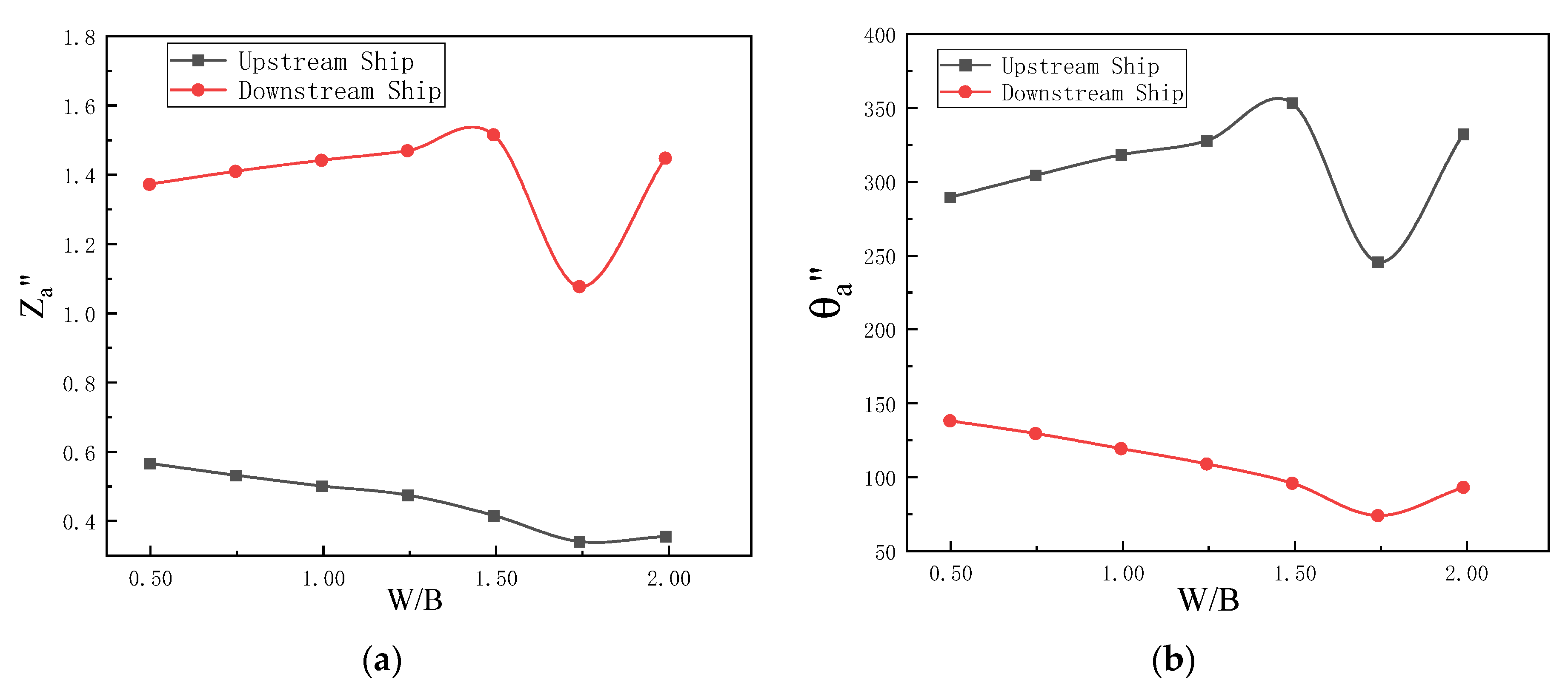
For salvage, the relative positions of the ships must be considered during the salvage process. If the distance is too small, collisions will occur between the vessels; however, if the distance is too large, the distance between the rescue vessel and the rescued vessel will be too large, resulting in normal rescue work not being carried out. The movement of the twin vessels at different distances is simulated, and the results are shown in Figure 10, where W/B is the ratio of the distance between the twin vessels to the vessel’s width. The numerical simulation of the model ship is carried out below under the conditions of zero speed, beam seas, wave length of 2.4 m and wave height of 0.024 m. To eliminate the effect of scale, the data are non-dimensionalised, and the main treatment is as follows:

$$z_a{}^{″}=z_a/A$$

(28)

$${\theta }_a{}^{″}=\frac{{\theta }_a}{kA}k=2\pi /\lambda$$

(29)

where A represents the wave amplitude, k is the wave number and $\lambda$ is the wave length.

When W/B < 1.5, as the distance between the twin ships increases, the amplitudes of the ships both move towards the two extremes—the original small amplitude decreases, and the amplitude of the motion of the twin ships scales linearly with the distance between the ships. However, for a distance of W/B > 1.5 between the two ships, the motion trend of the two ships changes; thus, W/B = 1.5 is the critical distance for the two ships to influence each other.

In the actual rescue process, the rescue vessel needs to approach the rescued vessel through its own motion. In this work, a lateral force is applied to the upstream vessel so that the vessel gains a velocity under the external force, which is used to simulate the process of the propeller pushing the vessel. Figure 11 shows a cloud of a two-dimensional ship model berthing with a velocity of Fr = 0.2 as a function of time. In practice, however, the relationship between how much force the ship needs to be propelled and the velocity between the force and the ship must be tested several times. The resulting relationship between force and ship velocity is shown in Figure 12, where the ship velocity is expressed in terms of the Froude number Fr, which is given by

$$\mathrm{F}\mathrm{r}=\frac{v}{\sqrt{gB}}$$

(30)

where v is the velocity of the ship. Again, the drag force is dimensionless. In Figure 12, due to the two-dimensional case, d denotes the ship’s height. There is basically a power function relationship between the velocity of the ship’s motion and the ship’s towing force.

The numerical simulation of the model ship was carried out under the conditions of beam seas, wave length of 2.4 m and wave height of 0.024 m. Figure 13 and Figure 14 show the motion response of the two vessels during the merging process and for a period of time after docking. After the upstream vessel has stopped, the RAO of the motion of the two vessels is essentially the same. The larger RAO is still at the lower velocity of the moving vessel.

3.2. Two-Ship Towing Study

In this section, we detail the seakeeping analysis of two ships during the towing process. Based on the three-dimensional potential flow theory, numerical simulations were carried out on the towing motion of the full-scale ship (116.95 m long). This section firstly simulates the appropriate wave direction for towing motion under the action of irregular waves (JONSWAP Spectrum). Secondly, under this wave direction, the influence of wave height and towing speed on the motion of the two boats is simulated. Before the simulation calculation, the external factors of the flow field need to be set first, including water depth and gravitational acceleration. Then, parameters such as hull weight, centre of gravity height and hull moment of inertia are modified. The ship model grid is shown in Figure 15. The grid has a total of 12,268 nodes and 12,000 cells.

To investigate the effect of different environmental conditions on the twin vessels, we first analysed the effect of different wave directions on the vessel motion by varying the wave direction. The sailing conditions of the twin boats at different wave depths are shown in

Table 2. Sailing conditions with different wave depths.

Wave Height	Spectral Peak Period	Current Velocity	Wind Velocity	Sailing Velocity	Cable Length
3 m	12 s	0.1 m/s	10 m/s	1 m/s	350.85 m

, where the cable length is 1.5 times the sum of the lengths of the front and back ships.

The yaw poles of the twin boats for different wave directions were first obtained, as shown in Figure 16. Due to the action of the cable, the difference in yaw poles between the two boats is not very large when sailing in most wave directions, with the yaw poles of the front boat being slightly larger than those of the rear boat. The yaw poles of the two boats are smaller in the following and head seas and larger in the oblique than in the beam seas, with the yaw poles reaching their maximum in the bow quartering seas, which is approximately twice as high as in the beam seas.

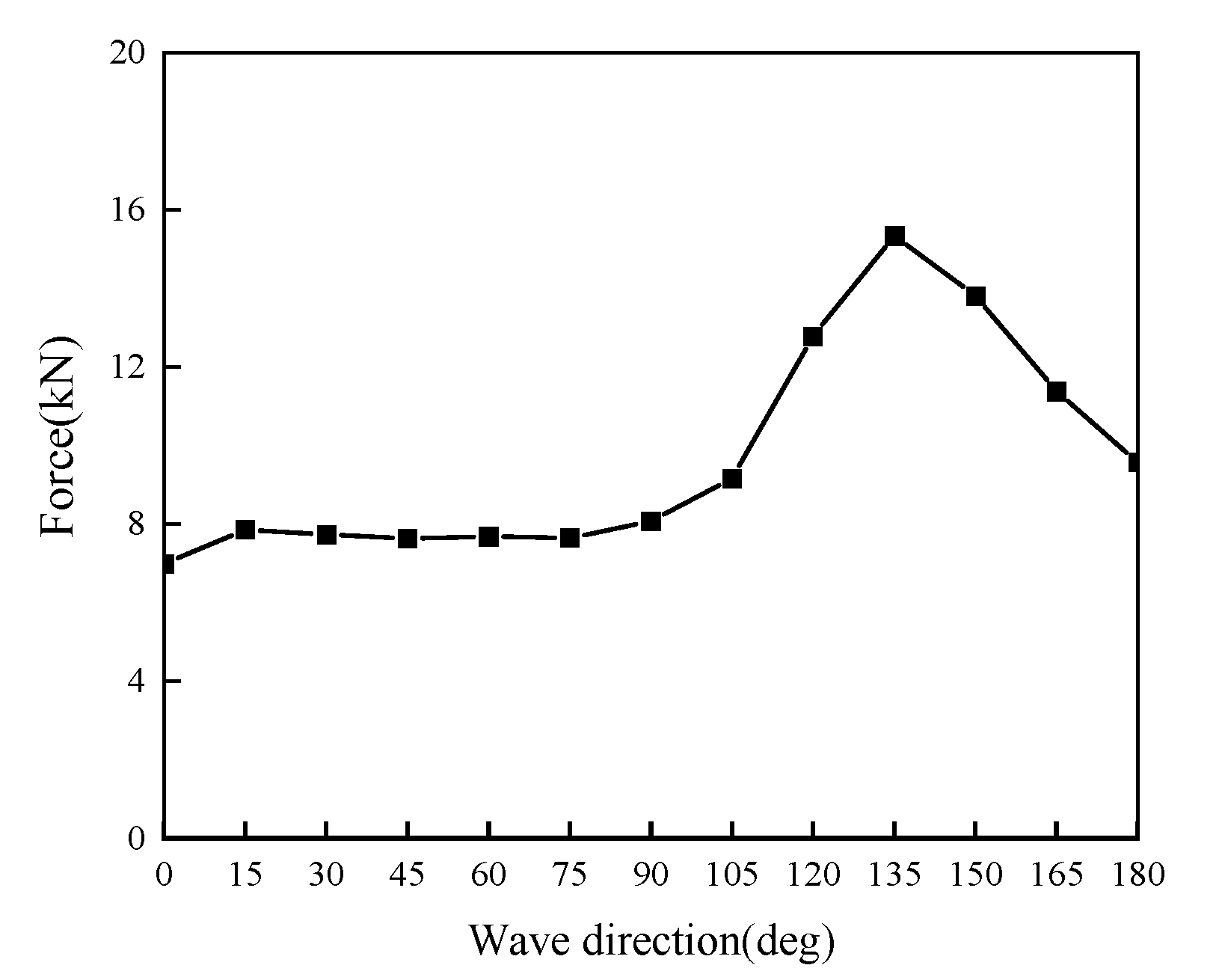
By calculating the roll, pitch and towing force response of the twin boats in different wave directions and averaging the absolute values of the data obtained, the curves of the average of the three degrees of freedom and the average of the towing force of the twin boats with wave direction can be obtained, as shown in Figure 17 and Figure 18.

It can be concluded from the observation curves that in the head seas condition, the twin boats have better heading stability and the three-degree-of-freedom response is smaller compared to other wave directions. In the wave direction range of 45°–135°, the stability of the twin boats is poor, with the bow and stern quartering seas having the greatest influence on the twin boats, and the average value of the roll and pitch the twin boats reaching the maximum. In the case of waves less than 90°, the loss of the front boat’s sheltering effect on the back boat results in the back boat’s pitch response being greater than that of the front boat, which is quite dangerous in the actual towing process, as the back boat is in a non-powered mode in most cases and cannot react quickly to changes in external conditions. When the wave direction is less than 90°, the towing force remains stable at approximately 8000 N and increases rapidly when the wave direction is greater than 90°, reaching a maximum value at 135°, after which the towing force gradually decreases. In summary, towing operations in rough sea conditions should be carried out in head seas as much as possible.

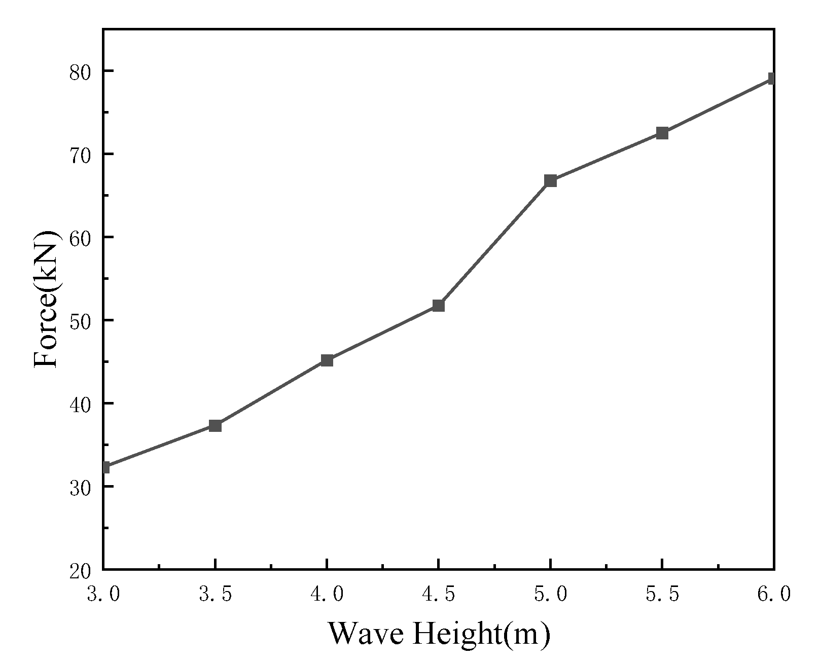
Therefore, according to the above conclusions, the numerical simulation is carried out under the conditions of head seas. For the external environment, in addition to the wave direction, the wave height also has an impact on the movement of the twin vessels. The effect of wave height on the motion of the two vessels is analysed here, and the motion response of the vessels is simulated for wave heights of 3–6 m (sea state 5–6). Other environmental conditions for the effect of wave height on the twin vessels are shown in

Table 3. Towing conditions at different wave heights.

Wave Direction	Spectral Peak Period	Current Velocity	Wind Velocity	Sailing Velocity	Cable Length
180°	8 s	0.2 m/s	15 m/s	5 m/s	350.85 m

.

The results of the numerical analysis of the freedom and the drag force were processed. The results are shown in Figure 19 and Figure 20.

It can be concluded from the observation curve that during the towing process against the waves, as the wave height increases, the average value of the roll of the two boats generally tends to increase, and the increase in the front boat is greater than that in the back boat. The average value of roll response at a wave height of 6 m is approximately 3–4 times higher than that at a wave height of 3 m. The four-degree-of-freedom response of the front boat is smoother than that of the back boat because the wave acts directly on the front boat and the front boat shades the back boat; therefore, the pitch curve of the front boat is more linear than that of the back boat. As the wave height increases, the towing force also increases, and the overall upward trend is consistent. In summary, when carrying out towing operations, we should try to choose sea conditions with lower wave heights for towing.

In addition to considering the impact of the external environment on the twin boats, it is also necessary to consider the factors of the twin boats themselves. The consideration is the towing velocity. We investigated the effect of a towing velocity of 1–7 m/s (corresponding to 0.5–3.5 knot velocity) on the twin vessels, and the remaining conditions are shown in

Table 4. Towing conditions at different towing velocities.

Wave Direction	Wave Height	Current Velocity	Wind Velocity	Spectral Peak Period	Cable Length
180°	3 m	0.2 m/s	15 m/s	8 s	350.85 m

.

Simulation calculations can result in the average value of the freedom as a function of velocity, as shown in Figure 21, and the average value of the towing force as a function of velocity, as shown in Figure 22.

By observing the curves, it can be concluded that during the towing process, the front boat has a certain shading effect on the rear boat, and the most obvious shading effect is the pitch curve. The average values of the pitch motion of the front boat and the rear boat differ greatly. The response of the roll and yaw motion of the two boats is not much different, but the roll and yaw of the front boat is always slightly larger than that of the rear boat. During the towing process, as the towing velocity increases, the four-degree-of-freedom response of the two vessels tends to generally rise, and as the velocity increases, the towing force on the towing cable also increases gradually and at an increasing rate. At a velocity of 1 m/s, the roll and yaw response of the two vessels is the largest. This is probably because the self-weight of the cable has a significant influence on the two vessels at low velocity, which leads to more severe ship rocking and thus affects the yaw response of the vessels, causing more serious yawing to occur. With increasing towing velocity, the average value of the towing force also increases, and with increasing velocity, the towing force is increasingly faster. At a velocity of 7 m/s, the average value of the towing force is approximately 3.5 times that at a velocity of 1 m/s. The average towing force at a speed of 7 m/s is approximately 3.5 times that at a speed of 1 m/s. Therefore, the speed range to be selected for a wave height of 3 m is 3–5 m/s.

3.3. Basin Test

Scaled-down ship model experiments are considered to be a reliable means of verification during ship simulation calculations. Many scholars have studied both real-scale and scaled-down ship models in many directions, such as kinematics and dynamics [20,21,22]. Although the scaled-down model of a ship may differ slightly from the actual values under certain conditions, in general, the experimental results of the scaled-down model are similar to the actual values and reflect the real situation of the ship relatively well.

The experiment was carried out in a basin with spherical wave-maker device. Regular waves are generated by the oscillation of a single wave ball, and irregular waves are generated by the combined motion of two wave balls. As shown in Figure 23, the wave basin is 50 m long, 30 m wide and 5 m deep, with a deep water area in the centre of the basin at a depth of 10 m, which is usually used to simulate deep water sea conditions. The ball wave basin is equipped with two symmetrically arranged wave balls on one side, which create waves through the up and down movement of the balls. The basic principle is that the motor pulls the elastic rope at the bottom of the wave ball to drive the ball in the vertical direction of movement. The movement of the ball causes the fluid around the ball to move, resulting in waves. The reflection of the basin wall and the superposition of the two wave spheres produces irregular waves similar to the actual marine environment. The instrument for measuring wave height measures the height of the water surface through the reflection of sound waves and then measures the real-time value of the wave. Taking the experiment of the twin vessel alongside test as an example, the twin vessel is arranged in the centre of the pool to reduce the influence of wall reflection on waves. The instrument for measuring wave height is located at the midpoint of the line connecting the centre of the wave-maker device and the ship’s centre.

The principle of instruments for measuring wave height is through the reflection of sound waves. The wave values are collected from the sound wave data reflected from the water surface. Take the data of measuring the approaching process of two boats as an example. The schematic diagram of the experimental site is shown in Figure 24. The blue dot in the picture represents the wave ball, and the yellow Pentagram represents the instrument that measures the wave height. A single wave-making ball moves up and down to generate waves, and the angle at which the waves hit the boats is controlled by pulling on a lightweight cable. The center of gravity of the two boats is about 10 m from the horizontal distance of the wave ball. A wave height measuring instrument is suspended at 5 m horizontally from the wave-making ball and 1.5 m from the water surface to measure the wave conditions around the ship. Other distances between the two boats and the wave ball can also be set, so the wave height data of more intervals around the boat can be measured. In addition, two wave-making balls move up and down to generate waves and then carry out the towing experiment of two boats, and the experimental principle is similar to the approaching process of two boats.

The ship model used for the test was a 3 m long scaled-down model, as shown in Figure 25, with the specific parameters shown in

Table 5. Parameters of the Wigley ship model.

Parameter	Wigley 3 m
Length of the boat	3 m
Beam	0.3 m
Draught line	0.1875 m
Dry side height	0.0925 m
Displacement Centre of gravity	74.98 m Z = −0.1354 m
Ixx	0.074
Iyy	1.421
Izz	1.430

. There is a 5 mm thick acrylic plate at the level of the centre of gravity to hold the attitude metre, sensors, counterweights and other equipment.

After the model is built, counterweights are placed inside the model to achieve its design weight, and the moment of inertia is adjusted by adjusting the position of the counterweights using a rotating inertia frame. The rotating inertia frame is shown in Figure 26. The upper part of the rotating inertia frame has two brackets, which are connected to the rotating inertia frame by pressure sensors to measure and control the position of the model’s centre of gravity. The lower part of the rotating inertia frame is the oscillating platform. The ratio of the difference between the oscillating period of the platform without the model and the oscillating period with the model and the height and weight of the ship is calculated to be equal to the rotating inertia of the model in the measurement direction. Furthermore, the oscillation DOF natural period for vessel scaled model is 0.212 s.

After completing the loading and levelling of the moulds, the moulds are lifted into the water via the overhead crane, and the twin vessels are tested alongside each other and towed separately.

3.3.1. Twin Vessel Alongside Test

The wave created by the wave sphere is a circular wave, which moves around the sphere and is superimposed by reflections when it meets the wall, forming an irregular wave with a random distribution of amplitude, but the wave period is the same as the movement frequency of the spheric wave-maker device and therefore remains basically the same. There are four wave patterns in the basin, and the actual wave conditions can be measured using a wave height meter. The four modes correspond to four different wave amplitudes, which are shown in

Table 6. Test wave parameters.

Mode	Amplitude (m)	Period (s)
a	0.0775	2.3116
b	0.0902	2.1501
c	0.1008	2.0032
d	0.1411	1.6778

.

According to the Froude number comparison, the four wave patterns have amplitudes of approximately 3 m, 3.5 m, 4 m and 5.5 m, respectively.

During the alongside test, the ship’s position is regulated by means of a lightweight rope, which allows the ship to be positioned in such a way that the relative position of the two ships is maintained and the relative angle between the ship and the wave sphere is ensured. After the vessel has reached its designated position, the rope is released. The amplitude of the ship’s motion in beam seas is measured for modes a, b and c. In d-mode, the twin boats produce the green sea phenomenon due to the high value of the wave height. As shown in Figure 27, when the twin boats are on the wave, it is mainly the bow that is on the wave; the degree of green sea phenomenon is small, and the water goes over the tip of the boat only. At this point, the middle and front of the twin boats are located in the trough of the wave, while the stern of the model is at the crest of the wave. The twin boats show a forward leaning posture, resulting in a lower relative position of the bow of the ship, and the water does not go over the bow, resulting in the green sea phenomenon of the bow of the ship. In addition, the ship’s roll motion is huge when the experiment in d-mode is performed, and the ship’s motion is also very unstable, resulting in inaccurate test data. Therefore, the ship’s motion response in d-mode was not tested to make the experiment safe and ensure the experimental data’s accuracy. In addition, the ship moves so violently in d-mode that it almost capsizes, as shown in Figure 28.

The following is a comparative analysis of the experiment and data simulation for different wave heights and distances between the two ships. Firstly, the response of the two ships under different wave heights is analysed. We take the ratio of wave height (H) to the total height of ship (d) as abscissa. The three points on each curve correspond to the heave and roll motions in modes a, b and c. Figure 29 shows the variation in the heave and roll amplitudes with the ratio of wave height (H) to the total ship height (d). It can be seen that the roll growth rate of the upstream ship is larger than that of the downstream ship, and the heave of the upstream ship is the opposite, which is consistent with the simulation. It can be seen that the values of heave and roll measured in the experiment are smaller than those in the numerical simulation. This is because the numerical simulation is carried out in the case of beam seas, but we cannot completely guarantee that the wave angle is 90° when conducting experiments. If the angle is greater or less than 90°, both the heave and the roll will be smaller.

Secondly, the response of the double boats at different distances is analysed. Figure 30 shows the variation in the heave and roll RAO of the two ships under different W/B values. It can be seen that the critical value for the apparent change in the moving trend of the two boats in the experimental curve is W/B equal to about 1.5, which is consistent with the conclusion of the numerical simulation. In general, the RAOs of the heave and roll measured experimentally are smaller than the RAOs of the numerical simulations because we cannot fully guarantee that the experiments are performed under beam seas.

3.3.2. Two-Ship Towing Test

The scaled-down model tests were mainly carried out for towing at different velocities and different wave heights.

The response of the towing system at different velocities is first analysed. According to the Froude number proposed in Section 3.1, when the model is reduced by a factor of $n$, its motion speed must be reduced by a factor of $\sqrt{n}$ simultaneously. From this, it can be calculated that when the speed of the 116.95 m long ship is 1–7 m/s, the movement speed of the 3 m model is 0.16–1.122 m/s. In addition, the experiment selects the same 3 m wave height as in the simulation, which corresponds to mode a. The wave height generated by mode a is 0.0775 m, the wave period is 2.3116 s and the same head seas condition is used in the simulation.

Figure 31 shows the experimental and numerical simulations of different speeds of roll, pitch and yaw. It can be seen that the front boat’s roll and pitch are more significant than those of the rear ship, mainly because the front boat has a specific shading effect on the rear ship, which is consistent with the conclusion drawn from the numerical simulation. Secondly, the roll and pitch measured in the experiment are more significant than the values in the numerical simulation. This may be because the tensile force generated by the motor used in the experiment fluctuates. Under the influence of the waves, the cable is sometimes tight and sometimes loose, which causes the front ship to have additional sway with the rear boat. This power cable significantly limits the yaw motion of the towing system, and the limitation of the length of the towing basin leads to a short towing time and a less significant yaw response.

Figure 32 shows the drag force test results at different speeds. The simulation results of the drag force at different velocities obtained in Section 3.2 are compared with the experimental results of the drag force obtained in this section by non-dimensional analysis and dividing by the maximum value of the drag force at different velocities, and the velocity value obtained by Froude number scaling was used as the horizontal coordinate to obtain the comparison curve between the simulation and the experimental results, as shown in Figure 33. The results of the simulation and the test are in agreement, which verifies the accuracy of the simulation results. In addition, the ratio of the experimentally measured towing force to the maximum supporting force is generally smaller than the numerical simulation value, which may be because the force provided by the experimental motor is unstable, so the tension sensor cannot always measure the normal value. However, the simulated ship is subject to constant tension at all times, so the ratio measured by the experiment is relatively small.

The towing test is then carried out with different wave heights; a, b and c wave modes were selected, corresponding to the simulated righteous wave heights of 3 m, 3.5 m and 4 m, and the towing velocity was selected as 0.801 m/s, corresponding to the simulated velocity of 5 m/s. The results of the roll, pitch and yaw are shown in Figure 34. The drag force results are shown in Figure 35. A comparison of simulated and experimental data by dividing the drag force by the maximum value at different wave heights is shown in Figure 36.

Comparing the test results with the simulation results in Section 3.2 reveals that the shading effect of the towing vessel on the towed vessel is most evident when conducting the towing tests at different wave heights. Whether it is an experiment or a numerical simulation, the roll and pitch of the front ship are larger than those of the back ship. As with the velocity comparison experiments, the yaw value of the towing system is smaller due to the limitations of the power cable and the towing site. As the wave height increases, the towing force of the towing system also increases. Similar to the simulation results, the average value of the towing force when H/d is 0.4 is approximately 1.7 times the average value when H/d is 0.25.

4. Conclusions

To ensure the safety of the rescue, we study the approaching process and the towing motion of the two ships. In this study, we performed seakeeping analysis of two ships during rescue operations. Based on viscous fluid and three-dimensional potential flow theory, numerical simulations were carried out on the side-by-side motion of the scaled ship model (3 m long) and the towing motion of the full-scale ship (116.95 m long). The main findings were obtained as follows.

Twin ship parallel study:

(1)

Numerical simulations of ships with wave heights of 0.024–0.132 m were carried out the condition of zero speed, beam seas, wavelength of 2.4 m, and the distance between two ships is the width of the ship. We found that the amplitude of the roll of the upstream vessel is greater than that of the downstream vessel, but the amplitude of heave of the downstream vessel is greater than that of the upstream vessel. The change in amplitude between the two vessels is mainly due to the change in flow direction of the fluid after it flows through the vessel, which leads to a change in the direction of the force on the downstream vessel. The change in force on the downstream vessel, in turn, leads to a change in the movement of the vessel, affecting both the fluid and the upstream vessel.

(2)

During the green sea phenomenon, the amplitude of the ship’s motion is generally larger due to the higher waves. And the green sea phenomenon is equivalent to adding ballast to the ship, which actually reduces the average amplitude of the ship’s motion.

(3)

Numerical simulations of ships with different distances between two ships were carried out under the conditions of zero speed, beam seas, the wavelength of 2.4 m, and wave height of 0.024 m. As the distance between the two ships increases, the amplitude of the motion between the two ships will relatively increase. A ratio of 1.5 times the width of the ship is the critical area where the motions of the two ships interact with each other, beyond which the amplitude of the ship’s motion will gradually return to the single-ship mode. For the berthing process, the faster the motion of the active vessel is, the lower the motion amplitude will be for both upstream and downstream vessels.

Two-ship towing study:

(4)

Different wave directions have a significant influence on the six degrees of freedom of the twin vessels. Especially in the interval of wave direction from 45° to 135°, the stability of the towing system is poor, and the response of the degrees of freedom and the response of the towing force of the twin vessels are at their maximum. When the wave direction is 180°, the stability of the towing system is relatively good. Towing operations should be carried out in head seas as far as possible.

(5)

Under the condition of head seas, the influence of wave height of 3–6 m (sea state 4–6) on ship motion is simulated. As the wave height increases, the overall response of the four degrees of freedom and the towing force of the towing system also increase, with the towing force and the roll response increasing more, while the pitch, heave and yaw response increase less. The towing system should choose the sea state with a smaller wave height for towing.

(6)

Under the condition of head seas and a wave height of 3 m, we continued to study the effect of towing speed on ship motion. We found that the influence of the towing velocity on the four degrees of freedom of the towing system is relatively small, but the influence on the change in the towing force is larger. With the increase in the towing velocity, the towing force also increased gradually and faster. However, when sailing at low velocity, the roll and yaw response of both boats are particularly large, so the most suitable velocity for towing should be 3 m/s to 5 m/s.

In the ship model test, based on the basin with a spherical wave-maker device and the scaled-down ship model, the experimental results show the same trend as the numerical simulation, which verifies the numerical simulation.

References

1. Shi, L. Research on the Towing Performance of Large Floating Bodies Based on AQWA. Master’s Thesis, Dalian University of Technology, Dalian, China, 2011. [Google Scholar]
2. Hong, S.Y.; Kim, J.H.; Cho, S.K.; Choi, Y.; Kim, Y. Numerical and experimental study on hydrodynamic interaction of side-by-side moored multiple vessels. Ocean. Eng. 2005, 32, 783–801. [Google Scholar]
3. Chen, X.B.; Malenica, S. Interaction hydrodynamique d’un ensemble de flotteurs sur la surface libre. 10emes J. L’hydrodynamique 2005, 1–14. [Google Scholar] [CrossRef]
4. Huang, W.; Li, B.; Chen, X.; Araujo, R. Numerical and experimental studies on dynamic gangway response between monohull flotel and FPSO in non-parallel side-by-side configuration. Ocean. Eng. 2018, 149, 341–357. [Google Scholar] [CrossRef]
5. Zhao, W.H.; Yang, J.M.; Hu, Z.Q. Hydrodynamic interaction between FLNG vessel and LNG carrier in side by side configuration. J. Hydrodyn. Ser. B 2012, 24, 648–657. [Google Scholar] [CrossRef]
6. Pessoa, J.; Fonseca, N.; Soares, C.G. Side-by-side FLNG and shuttle tanker linear and second order low frequency wave induced dynamics. Ocean. Eng. 2016, 111, 234–253. [Google Scholar] [CrossRef]
7. Nam, B.W.; Kim, Y.; Hong, S.Y. Time-domain simulation of berthing problem between FPSO and shuttle tanker in waves. Ocean. Res. 2016, 58, 49–61. [Google Scholar]
8. Yue, J.; Kang, W.; Mao, W.; Chen, P.; Wang, X. Prediction of dynamic responses of FSRU-LNGC side-by-side mooring system. Ocean. Eng. 2020, 195, 1–15. [Google Scholar]
9. Xu, L.-Y. Research on Hydrodynamic Disturbance of Multi-Floating Bodies. Master’s Thesis, Shanghai Jiaotong University, Shanghai, China, 2014. [Google Scholar]
10. Gao, Z.; Wang, Y.; Su, Y. On damaged ship motion and capsizing in beam waves due to sudden water ingress using the RANS method. Appl. Ocean. Res. 2020, 95, 102047. [Google Scholar]
11. Shen, Z.; Cao, H.; Ye, H.; Liu, Y.; Wan, D.C. Development of CFD Solver for Ship and Ocean Engineering Flows. In Proceedings of the 8th International OpenFOAM Workshop, The International Convention Center (ICC), Jeju, Korea, 11–14 June 2013. [Google Scholar]
12. Ye, H.; Shen, Z.; Wan, D. Computational analysis of container ships with large movements in waves. In Proceedings of the 11th National Hydrodynamics Conference and the 24th National Hydrodynamics Symposium and the 110th Anniversary of Zhou Peiyuan’s Birth, Wuxi, China, 25–29 August 2012. [Google Scholar]
13. Wang, J.; Wan, D.C. Numerical simulation of pure rocking head motion of a ship based on overlapping mesh technique. Hydrodyn. Res. Prog. Ser. A 2016, 31, 567–574. [Google Scholar]
14. Wang, J.; Wan, D.C. Investigations of Self-Propulsion in Waves of Fully Appended ONR Tumblehome Model. Math. Mech. 2016, 37, 1345–1358. [Google Scholar]
15. Wang, J.H.; Wan, D.C. CFD numerical simulation of the slewing maneuvering motion of a ship in waves. China Ship Res. 2019, 14, 1–8. [Google Scholar]
16. 16. Zhirong. S. Numerical Method Study of Overlapping Mesh Technique for Ship Paddle-Rudder Interaction. Ph.D. Thesis, Shanghai Jiaotong University, Shanghai, China, 2014.
17. Journée, J.M.J. Experiments and Calculations on 4 Wigley Hull Forms in Head Seas. In Delft University of Technology Report; Delft University of Technology: Delft, The Netherlands, 1992. [Google Scholar]
18. Chen, Y. Numerical Simulation of the Interaction between Isolated Waves and Submerged Bodies in the Ocean. Master’s Thesis, South China University of Technology, Guangzhou, China, 2010. [Google Scholar]
19. Zhang, Q. Numerical Simulation of Nonlinear Wave Impact through Hollow Structures. Master’s Thesis, Zhejiang University, Hangzhou, China, 2008. [Google Scholar]
20. Lin, Y.C.; Earls, C.J.; Park, J.T.; Smith, T.C. Stochastic inversion for the roll gyradius second moment mass property in ships at full-scale and model-scale. Ocean. Res. 2017, 63, 24–35. [Google Scholar] [CrossRef]
21. Chen, Y.; Tong, Z.P.; Hua, H.X.; Wang, Y.; Gou, H.Y. Experimental investigation on the dynamic response of scaled ship model with rubber sandwich coatings subjected to underwater explosion. Int. J. Impact Eng. 2009, 36, 318–328. [Google Scholar] [CrossRef]
22. Terziev, M.; Tezdogan, T.; Demirel, Y.K.; Villa, D.; Mizzi, S.; Incecik, A. Exploring the effects of velocity and scale on a ship’s form factor using CFD. Int. J. Nav. Archit. Ocean. Eng. 2021, 13, 147–162. [Google Scholar] [CrossRef]
Figure 1. Wigley ship model.
Jmse 10 01209 g001
Figure 2. Schematic diagram of the two-dimensional flow field.
Jmse 10 01209 g002
Figure 3. Two-dimensional flow field meshing: (a) meshing of ships and their fluid domains, (b) grid around the ship after nesting and (c) grid of the entire flow field after nesting.
Jmse 10 01209 g003
Figure 4. Grid independence of two-dimensional grids.
Jmse 10 01209 g004
Figure 5. Two-dimensional numerical simulation of twin ship motion clouds.
Jmse 10 01209 g005
Figure 6. Double boat movement over time: (a) heave and (b) roll.
Jmse 10 01209 g006
Figure 7. Response of two boats at different wave heights: (a) roll amplitude, (b) heave amplitude.
Jmse 10 01209 g007
Figure 8. Cloud atlas of the green sea phenomenon.
Jmse 10 01209 g008
Figure 9. Two-ship amplitude response during green sea phenomenon: (a) heave amplitude, (b) roll amplitude.
Jmse 10 01209 g009
Figure 10. The effect of different distances on the movement of the vessel: (a) heave RAO and (b) roll RAO.
Jmse 10 01209 g010
Figure 11. Two-dimensional ship berthing process cloud.
Jmse 10 01209 g011
Figure 12. Relationship between vessel forces and the lateral berthing velocity.
Jmse 10 01209 g012
Figure 13. Vessel motion response at different velocities during berthing: (a) heave RAO and (b) roll RAO.
Jmse 10 01209 g013
Figure 14. The RAO of the ship’s motion after stopping at different velocities: (a) heave RAO and (b) roll RAO.
Jmse 10 01209 g014
Figure 15. Ship model meshing.
Jmse 10 01209 g015
Figure 16. Variation in yaw poles with wave direction for twin ships.
Jmse 10 01209 g016
Figure 17. Variation in the mean value of freedom with wave direction: (a) roll, (b) pitch.
Jmse 10 01209 g017
Figure 18. Variation in the mean drag force with the wave direction.
Jmse 10 01209 g018
Figure 19. Variation in the mean value of the freedom with wave height: (a) roll, (b) pitch, (c) yaw.
Jmse 10 01209 g019
Figure 20. Variation in the mean drag force with wave height.
Jmse 10 01209 g020
Figure 21. Variation in the mean value of the freedom with towing velocity: (a) roll, (b) pitch, (c) yaw.
Jmse 10 01209 g021
Figure 22. Variation in the average towing force with towing velocity.
Jmse 10 01209 g022
Figure 23. Wave-making basin.
Jmse 10 01209 g023
Figure 24. The schematic diagram of the experimental site of the approaching process.
Jmse 10 01209 g024
Figure 25. Wigley ship model.
Jmse 10 01209 g025
Figure 26. Rotating inertia frame.
Jmse 10 01209 g026
Figure 27. The state of the ship in the green sea phenomenon in d-mode: (a) state of the experiment; (b) state in numerical simulation.
Jmse 10 01209 g027
Figure 28. The state of vigorous motion of the ship in d-mode.
Jmse 10 01209 g028
Figure 29. Numerical and experimental value of the freedom with wave height (H/d): (a) roll, (b) heave.
Jmse 10 01209 g029
Figure 30. Numerical and experimental value of the freedom with W/B: (a) roll RAO, (b) heave RAO.
Jmse 10 01209 g030
Figure 31. Numerical and experimental values of the freedom with Fr: (a) roll, (b) pitch, (c) yaw.
Jmse 10 01209 g031aJmse 10 01209 g031b
Figure 32. Drag force test results at different Fr values.
Jmse 10 01209 g032
Figure 33. Comparison of simulation and test results.
Jmse 10 01209 g033
Figure 34. Numerical and experimental values of the freedom with wave heights (H/d): (a) roll, (b) pitch, (c) yaw.
Jmse 10 01209 g034aJmse 10 01209 g034b
Figure 35. Drag force test results at different wave heights (H/d).
Jmse 10 01209 g035
Figure 36. Comparison of simulation and test results.
Jmse 10 01209 g036