Hydrodynamic Performance of a Catamaran in Shallow Waters

Abstract

The effects of limited water depth on the hydrodynamic performance of a catamaran with the full-scale dimensions and geometry of a WAM-V 16 unmanned surface vehicle operating in shallow waters are investigated using an incompressible URANS-VOF solver in OpenFOAM^®. Simulations of the flow associated with the passage of the catamaran in shallow waters have been conducted for a range of vehicle speed and several shallow to intermediate water depths under free trim and sinkage conditions. The effects of water depth on the resistance and the dynamic motion of the catamaran are characterized. The total resistance coefficient of the catamaran is shown to increase by as much as over 40% at transcritical Froude numbers, close to the critical depth-dependent Froude number ($F{r}_h=1.0$). The wave system associated with the flow is examined and its relationship to observed impacts on resistance, trim and sinkage are discussed. The effect of limited water depth on Kelvin’s wake angle is characterized in terms of both length and depth Froude numbers and is shown to be in good agreement with theory.

1. Introduction

A catamaran offers good transverse stability and increased payload capacity while operating at high speeds. Studies of the hydrodynamic factors governing the resistance and seakeeping properties of a catamaran are therefore of interest. For operation in shallow waters, there is interest in understanding the impact of the interaction between the hull and the seabed on the total resistance, trim, and sinkage that affect the catamaran’s maneuvering capabilities. Conventional ships monitor the water depth when in shallow waters for safe navigation, avoiding grounding and squatting. The flow past a catamaran in motion in calm water is characterized by the boundary layer, wake, and transverse and divergent wave patterns associated with each demihull, and the interference between them. For a catamaran of length $L_{PP}$ moving at speed U in water of depth h, the flow is typically parameterized in terms of a vehicle length-based Froude number, ($Fr=U/\sqrt{g{L}_{PP}}$), a depth-based Froude number ($F{r}_h=U/\sqrt{gh}$) and Reynolds number $Re$; here g is gravitational acceleration. In shallow water, for ($F{r}_h\approx 1.0$), resistance, trim and sinkage of the catamaran are significantly amplified [1]. The value $F{r}_h=1.0$ is therefore referred to as the critical Froude number.

Several experimental studies have considered the dependence of the resistance and dynamic motion of catamarans in calm water on hull geometry, demihull beam-to-length ratio $B/L_{PP}$, demihull beam-to-draft ratio $B/T$, hull separation-to-length ratio $S/L_{PP}$, and length and depth-based Froude numbers $Fr$, and $F{r}_h$. Insel and Molland [2] investigated the deep-water motion of a series of high-speed catamarans for several values of $S/L_{PP}$ and $B/L_{PP}$. Viscous and wave-making contributions of resistance were determined for a range of $Fr$, both observed to depend principally on $B/L_{PP}$ and the extent of the flow separation. In general, the interference between the hulls led to increase in the total resistance coefficient $C_T$, particularly over the critical and super critical range of $Fr$. Similar results were obtained by other notable deep-water investigations, including [3,4,5,6]. van’t Veer [3] and Broglia et al. [6] respectively investigated the seakeeping and resistance performances of Delft 372 catamaran, which has been widely used for benchmark purposes, for various hull separation ratios $S/L_{PP}$ over a range of $Fr$. Interference effects on the resistance were observed for $Fr>0.3$, reaching maximum at $Fr\approx 0.5$. Strong correlation between interference resistance and trim and sinkage of the catamaran was noted. Souto-Iglesias et al. [4] investigated the wave field between the demihulls and its effect on the interference resistance. Subsequently, Souto-Iglesias et al. [5] investigated the interference effects of fixed and free models of a Series 60 catamaran, finding that the free or fixed model conditions did not affect the interference substantially.

Molland et al. [7,8] extended the deep-water experimental investigation reported in [2] to shallow water. They observed a distinct increase in the resistance coefficient $C_T$ in the subcritical to critical depth Froude Number, the increase being larger for the smaller of the two water depths considered, suggesting that the proximity of the seabed adversely affects the total resistance. Lee et al. [9] experimentally investigated the hydrodynamic performance of a CATA IV catamaran for a range of values of $S/L_{PP}$ in deep and shallow waters. Consistent with [7,8], they observed that the measured resistance in shallow water exceeded that in deep water in the sub-critical to critical $Fr$ range but was lower than in deep water for supercritical values of $Fr$. The effects were accentuated as $S/L_{PP}$ was reduced. Zlatev et al. [10] conducted additional experiments with the Delft 372 catamaran model in shallow waters, the results of which are consistent with these findings. Similar results were reported by Dand et al. [11] in their investigation of a catamaran sailboat. Subsequently, Falchi et al. [12] investigated the dynamics of the vortices generated by the Delft 372 catamaran and their interactions with the wave patterns using stereo-PIV measurements.

Linear, slender hull and potential flow based theory [13,14,15] provides good predictions of the characteristics of the non-viscous contributions to resistance and wave distribution. It serves as a useful design tool in early stage of the design process in exploring appropriate combinations of hull parameters and hull spacing. To capture the viscous contributions, consideration of the full Navier Stokes equations is needed. Several computational fluid dynamic (CFD) studies of the catamaran motion in deep water have been carried out via commercial and open-source solvers based on unsteady Reynolds averaged Navier Stokes (URANS) equations. Notable studies include those by Zaghi et al. [16], Broglia et al. [17], and He et al. [18], all of whom studied the hydrodynamics of the Delft 372 catamaran model, Haase et al. [19] who considered a large-medium speed catamaran, and Farkas et al. [20] who studied the hydrodynamics of a series 60 catamaran. Consistent with experimental results and potential flow theory, these investigations find that in deep water the total resistance coefficient $C_T$ of a catamaran as a function of $Fr$ typically exhibits two peaks, with the second peak at a higher value of $Fr$ being larger than the first. Zaghi et al. [16] coupled experimental results with a CFD analysis of the flow field around the catamaran and showed that the two peaks occur when a wave trough is at the stern. The second peak was found to be associated with strong interference effects that increase as $S/L_{PP}$ is reduced. Broglia et al. [17] applied URANS approach to examine the interference effects on the surface of the Delft 372 catamaran in terms of the distribution of streamlines, cross flows, pressure and wave patterns. The computations suggested minimal influence of the Reynolds number $Re$ on the interference effects. Haase et al. [19] developed a novel method for predicting full-scale resistance of a large-medium speed catamaran that is based on verification using model scale experiments and including surface roughness effects. Farkas et al. [20] conducted numerical simulations of the Series 60 catamaran model and investigated the wave and viscous components of hull interference. The results suggested that the form factor was effectively independent of $Fr$ but depended on the hull separation distance $S/L_{PP}$.

Notable fully viscous CFD studies of catamaran hydrodynamics in shallow water include those by Castiglione et al. [21] (See also [22]), and by Shi et al. [23]. Castiglione et al. [21] used URANS code CFDSHIP-Iowa V.4 and Shi et al. [23] used the commercial URANS code Star CCM+ 14.06 in their studies. In [21], the Delft 372 catamaran was considered and the results for resistance, trim and sinkage were shown to be in good agreement with experimental results reported in [3], and [10]. A number of subsequent papers relating to various aspects of the hydrodynamic of Delft 372 catamaran have been published and are comprehensively documented by Broglia et al. [24]. Shi et al. [23] computed the resistance of a full-scale zero-emission catamaran in both deep and shallow waters and demonstrated that the overall characteristics of the total drag coefficient for the vehicle were consistent with those determined experimentally for similar catamarans.

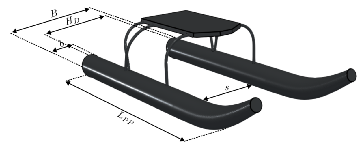
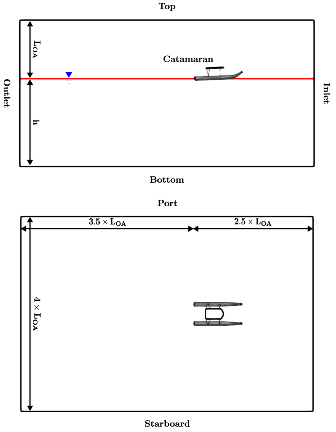
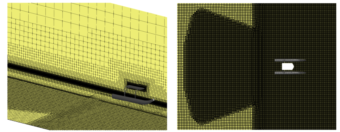
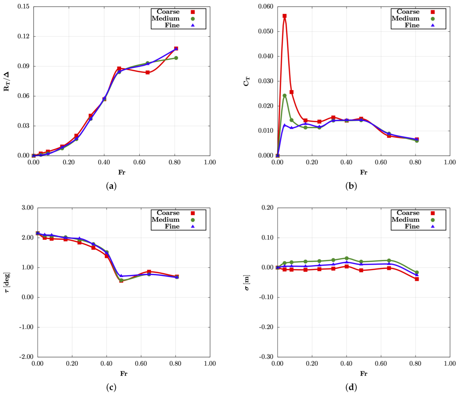
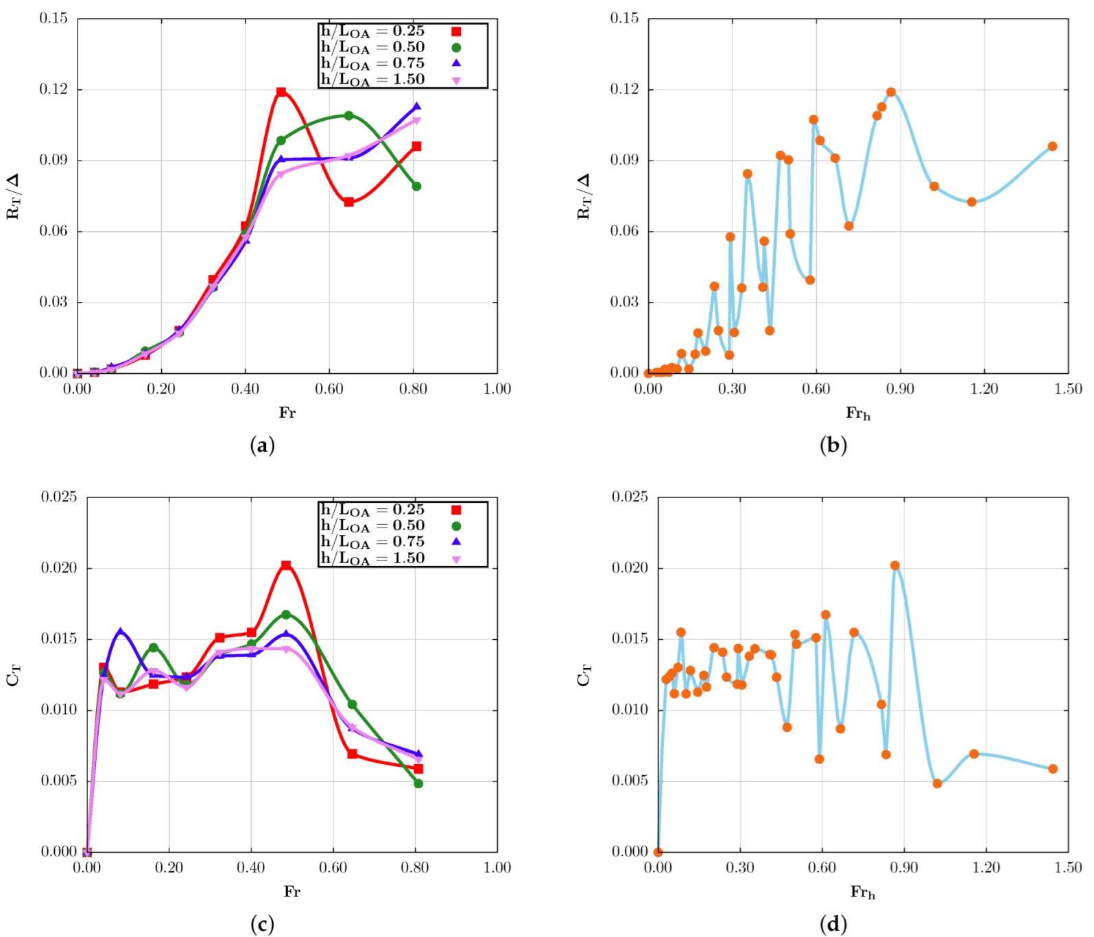
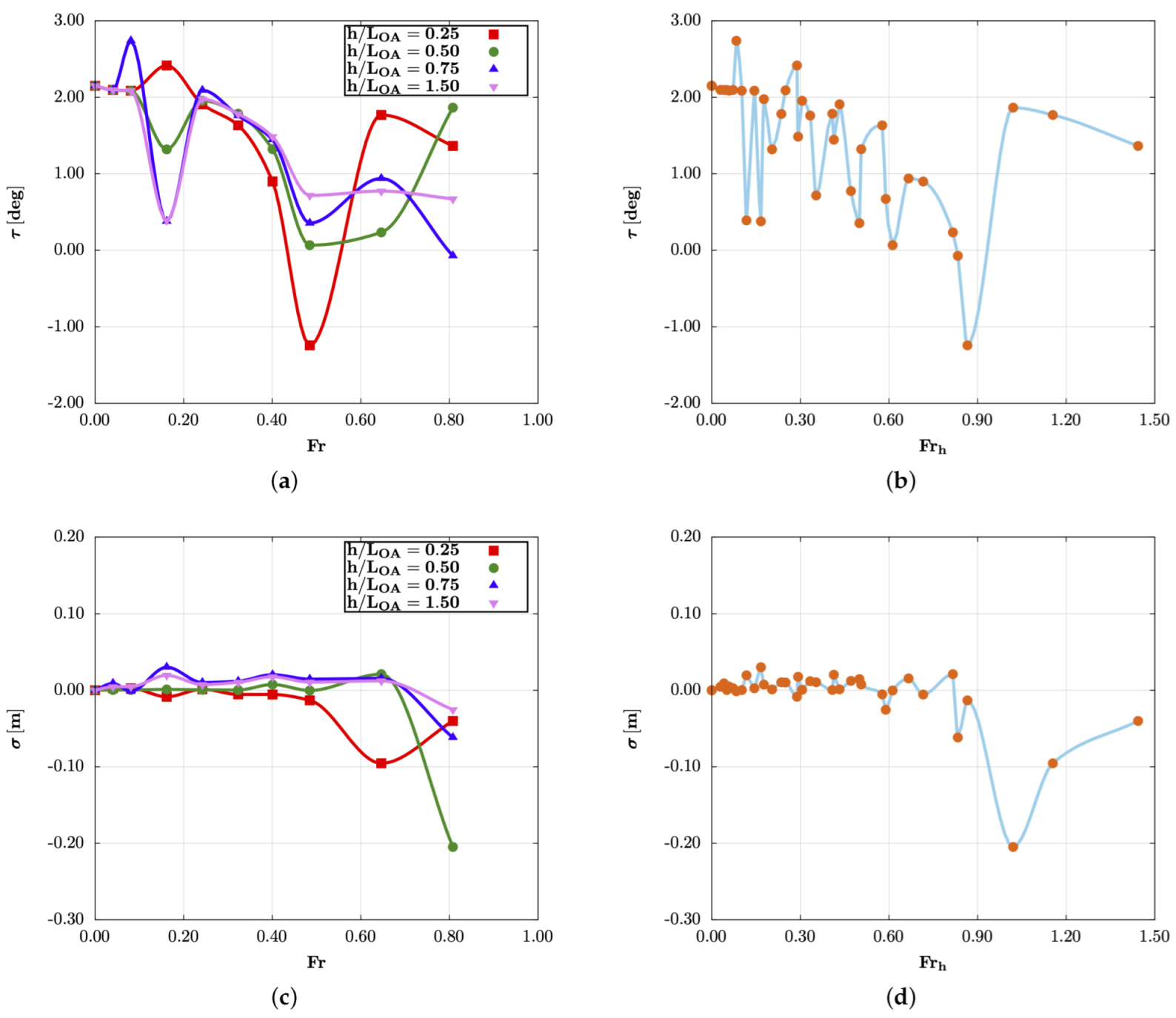
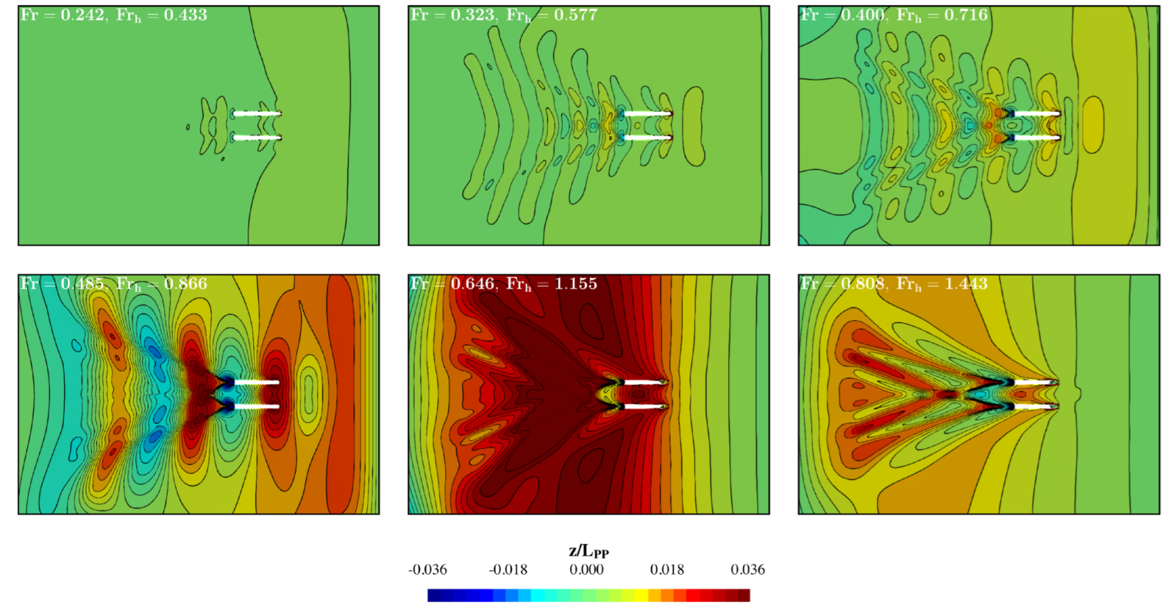
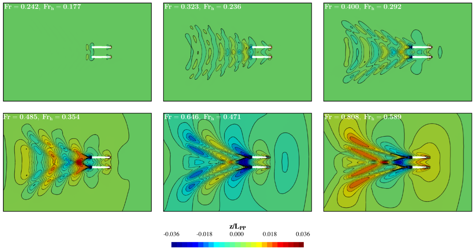
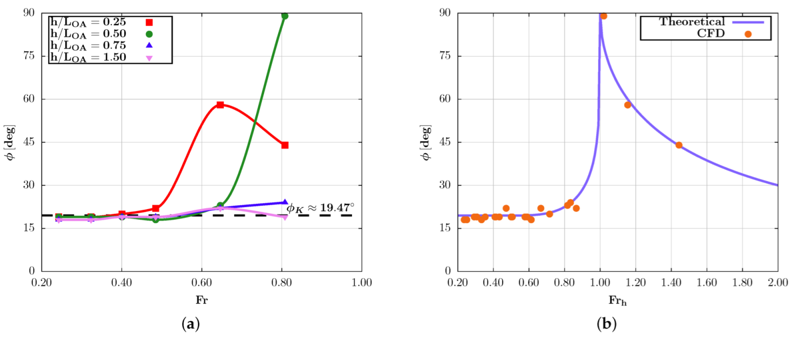
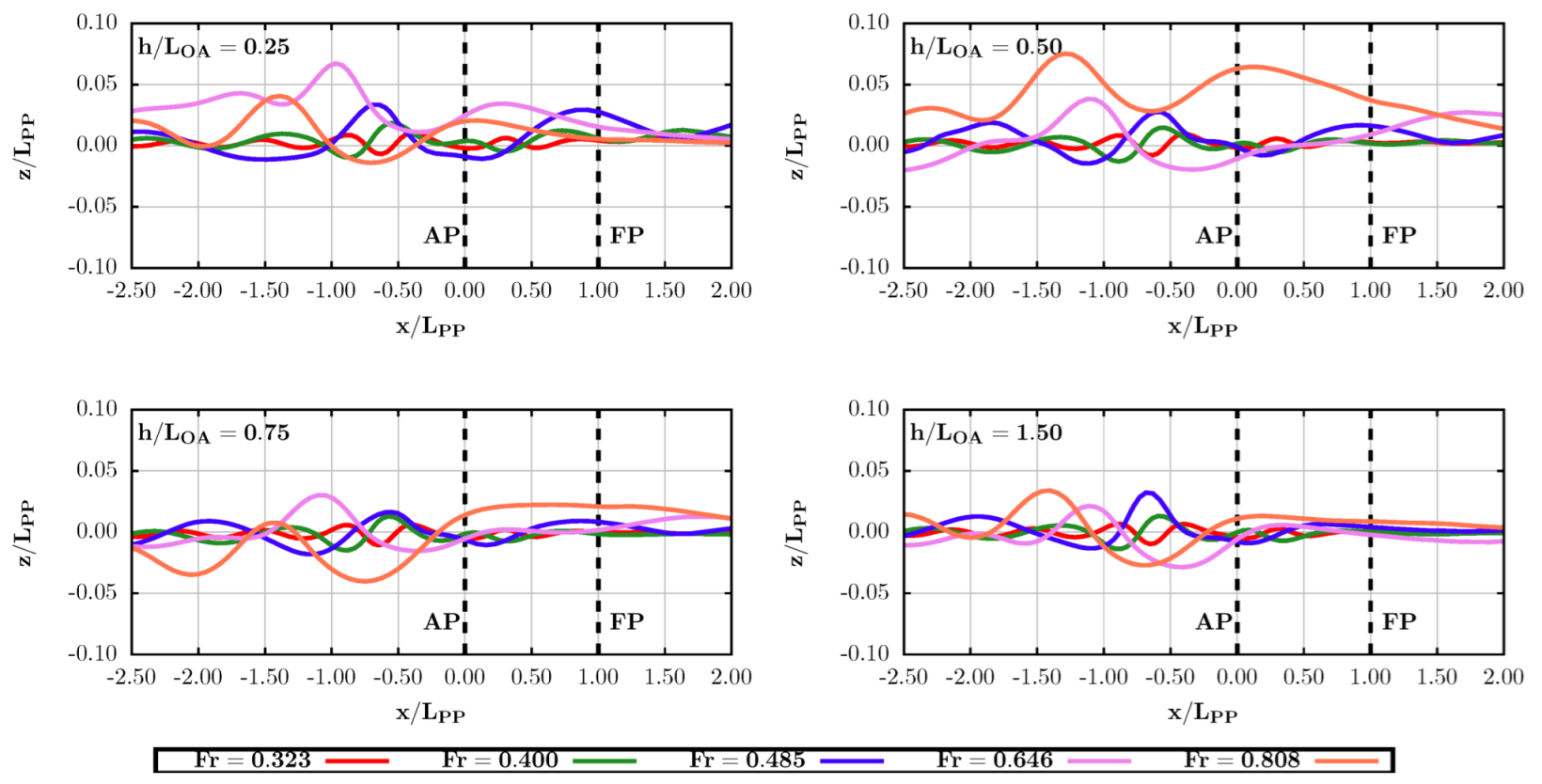
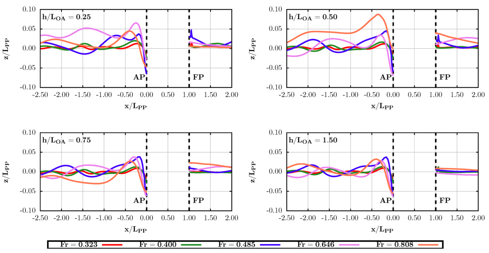
In the URANS-based study described here, we have investigated the hydrodynamic performance of a full-scale catamaran with dimensions and geometry corresponding to a Wave-Adaptive-Modular-Vehicle (WAM-V 16) catamaran operating in shallow waters for Froude numbers in the range $0.05<Fr<0.8$ using OpenFOAM-v2106^® (Open Field Operation and Manipulation). WAM-V 16 catamarans are being utilized as unmanned surface vehicles (USVs), and the study is in support of developing autonomous control systems for the vehicles while operating in shallow coastal waters. We include consideration of a range of intermediate depths and do not assume symmetry about the catamaran center-line. While the latter requires computing the whole domain, it facilitates extending the CFD code to consider roll and sway motion of the catamaran and operations in oblique waves. Additionally, no-slip boundary condition is applied on the bottom boundary to allow proper consideration of the viscous effects in shallow waters. The objective of the current study is to characterize the effects of limited water depth on the resistance, trim, sinkage and wave interference between the demihulls as functions of $Fr$. The wave field generated by the catamaran is examined and its relationship to observed impacts on resistance, trim and sinkage are discussed. Finally, we examine the characteristics of the Kelvin angle of the catamaran’s wake in terms of both $Fr$ and $F{r}_h$.

2. Mathematical Modeling

2.1. Governing Equations of Fluid Motion

The unsteady Reynolds Averaged (URANS) equations of motion for viscous, incompressible fluid flow are given by:

$$\nabla ·\overline{\mathbf{U}}=0$$

(1)

$$\rho \frac{\partial \overline{\mathbf{U}}}{\partial t}+\rho \nabla ·\left(\overline{\mathbf{U}}\otimes \overline{\mathbf{U}}\right)=\rho \mathbf{g}-\nabla \overline{p^{\prime }}+2\nabla ·\mu \nabla \overline{\mathbf{S}}-\nabla ·\left(\rho {\overline{\mathbf{R}}}_{\mathrm{dev}}\right)$$

(2)

in which $\overline{p^{\prime }}$ is the modified mean pressure given by

$$\overline{p^{\prime }}=\overline{p}+\frac{2}{3}\rho k,$$

(3)

$\overline{\mathbf{S}}$ is the mean rate of strain,

$$\overline{\mathbf{S}}=\frac{1}{2}\left[\nabla \overline{\mathbf{U}}+\nabla {\left(\overline{\mathbf{U}}\right)}^T\right],$$

(4)

and ${\overline{\mathbf{R}}}_{\mathrm{dev}}$ is the deviatoric anisotropic stress tensor given by

$${\overline{\mathbf{R}}}_{\mathrm{dev}}=\overline{{\mathbf{U}}^{\prime }\otimes {\mathbf{U}}^{\prime }}-\frac{2}{3}k\mathbf{I}.$$

(5)

Here, $\overline{\mathbf{U}}$ is the mean component of the fluid velocity, $\rho$ is the fluid density, $\mathbf{g}$ is the gravitational acceleration vector, $\mu$ is the dynamic viscosity of the fluid, $\mathbf{I}$ is the identity matrix, and $k=\frac{1}{2}\overline{U^{\prime }·U^{\prime }}$ is the kinetic energy of turbulent fluctuations.

2.2. Volume of Fluid (VOF) Method

The Volume of Fluid (VOF) method is used to track the air-water interface. Thus, the volume of fluid of every mesh cell in the computational domain is assigned a scalar phase fraction function $\alpha$ that characterizes the fraction of the cell volume occupied by water. When a cell is completely filled with water, $\alpha =1$, when it is completely filled with air, $\alpha =0$. The air-water interface is defined by the cells that are partially filled with water and are therefore characterized by $0<\alpha <1$ [25]. That is,

$$\alpha =\left\{\begin{array}{cc}0& \mathrm{air}\\ 0<\alpha <1& \mathrm{interface}\\ 1& \mathrm{water}\end{array}\right.$$

(6)

The volume phase fraction $\alpha$ of every air and water cell in the computational mesh is tracked. Both fluids share a single set of momentum equations, with the physical properties of the fluid for each cell computed as weighted averages based on the phase fraction distribution. Thus,

$$\rho ={\rho }_w\alpha +{\rho }_a\left(1-\alpha \right),$$

(7)

$$\mu ={\mu }_w\alpha +{\mu }_a\left(1-\alpha \right).$$

(8)

We follow [26] in specifying the transport equation for $\alpha$ as

$$\frac{\partial \alpha }{\partial t}+\nabla ·\left(\mathbf{U}\alpha \right)+\nabla ·\left[{\mathbf{U}}_C\alpha \left(1-\alpha \right)\right]$$

(9)

where

$$\mathbf{U}=\alpha {\mathbf{U}}_w+\left(1-\alpha \right){\mathbf{U}}_a$$

(10)

and ${\mathbf{U}}_c={\mathbf{U}}_w-{\mathbf{U}}_a$. The last term in Equation (9) is an artificial compression term, with ${\mathbf{U}}_c$ representing a “compression velocity” vector, which enables sharp resolution of the interface through compression. Equation (9) is solved simultaneously with the equations of motion. The approach in [26] overcomes difficulties in maintaining conservation and boundedness of $\alpha$ in the conventional VOF method that are known to lead to errors in the computation of the physical properties of the fluids [27,28,29,30]. Accurate computation of the phase fraction by the approach also enables accurate estimation of the surface curvature that is needed for computing surface tension and pressure gradient at the free surface. The compression term only applies to the interface region, and it dissipates at the boundaries of the phase fraction. The formulation eliminates the need of a high-resolution scheme for phase fraction and enables capturing a higher resolution interface compared with the conventional VOF approach. Due to the nature of this problem, numerical diffusion inevitably occurs, which can be avoided by using an appropriate discretization method for the convection term. The boundedness of Equation (9) is achieved by a solver called MULES (multidimensional universal limiter for explicit solution). MULES uses a limiting factor on the fluxes to ensure the final value of phase fraction is between 0 and 1 [31].

2.3. Turbulence Modeling

Using the Boussinesq hypothesis [32], we assume that the Reynolds stress, $-\rho {\overline{\mathbf{R}}}_{\mathrm{dev}}$ in (2) is proportional to the mean rate of strain,

$$-\rho {\overline{\mathbf{R}}}_{\mathrm{dev}}=2{\mu }_t\overline{\mathbf{S}}$$

(11)

where $\overline{\mathbf{S}}$ is given by (4) and ${\mu }_t$ is the dynamic eddy viscosity. Thus the momentum Equation (2) for the mean flow become:

$$\rho \frac{\partial \overline{\mathbf{U}}}{\partial t}+\rho \nabla ·\left(\overline{\mathbf{U}}\otimes \overline{\mathbf{U}}\right)=\rho \mathbf{g}-\nabla \overline{p^{\prime }}+2\nabla ·(\mu +{\mu }_t)\nabla \overline{\mathbf{S}}$$

(12)

Here, we adopt the Shear Stress Transport (SST) $k-\omega$ turbulence model [33] for incompressible flows to model the dynamic eddy viscosity in view of its robustness and adequate treatment of boundary layers, including accurate wake predictions in high-Reynolds number flows around ship hulls [34]. Thus,

$${\mu }_t=a_1\rho \frac{k}{max\left(a_1\omega ,b_1{F}_{23}\mathbf{S}\right)}$$

(13)

where $a_1$, $b_1$, and $F_{23}$ are constants and the turbulent kinetic energy, k, and the specific dissipation rate, $\omega$, satisfy the transport equations:

$$\frac{\mathrm{D}}{\mathrm{D}t}\left(\rho k\right)=\nabla ·\left(D_k\nabla k\right)+\rho G-\frac{2}{3}\rho k-\rho {\beta }^{*}\omega k+S_k$$

(14)

$$\frac{\mathrm{D}}{\mathrm{D}t}\left(\rho \omega \right)=\nabla ·\left(\rho D_{\omega }\nabla \omega \right)+\frac{\rho \gamma G}{\nu }-\rho \beta {\omega }^2-\rho \left(F_1-1\right)C{D}_{k\omega }+S_{\omega }$$

(15)

Expressions for $D_k$, $D_{\omega }$, $S_k$, G, $C{D}_{k\omega }$, together with the constants, $a_1$, $b_1$, $F_{23}$$F_1$, $\beta$, $\beta *$, and $\gamma$ are provided in the Appendix A. The model switches adaptively between the $k-ϵ$ model in the far field and the $k-\omega$ model inside turbulent boundary layers, assigning appropriate values to the constants in the above equations using blending functions [32]. The two transport Equations (14) and (15) are solved simultaneously with (9) and (12).

2.4. Equations of 6-DOF Motion and Coordinate System

The forces and moments acting on the vehicle are determined through solution of Equations (1) and (2) for the fluid flow and computing the viscous and pressure forces on the vehicle, integrating them over the body as

$$\mathbf{F}={\int }_S\left(\tau -p\mathbf{I}\right)\mathbf{n}·\mathrm{d}S-m\mathbf{g}$$

(16)

$$\mathbf{M}={\int }_S\left(\mathbf{R}-{\mathbf{R}}_{\mathbf{CG}}\right)\times \left(\tau -p\mathbf{I}\right)\mathbf{n}·\mathrm{d}S$$

(17)

in which $\tau$ represents the shear stress force acting on the catamaran, $\mathbf{n}$ is the surface normal vector, $\mathbf{R}$ is the position vector of the points located on the surface of the catamaran and ${\mathbf{R}}_{\mathbf{CG}}$ is the position vector of the center of gravity of the catamaran.

The computed forces and moments on the vehicle are used to determine the 6-DOF motion of the vehicle using

$$\frac{\mathrm{d}}{\mathrm{d}t}\left(m{\mathbf{U}}_{\mathbf{CG}}\right)=\mathbf{F}$$

(18)

$$\frac{\mathrm{d}}{\mathrm{d}t}\left({\mathbf{I}}_{\mathbf{CG}}·{\mathit{\omega }}_{\mathbf{CG}}\right)=\mathbf{M}$$

(19)

Here the 6-DOF motion refers to the rotational and translational motions defined about the three axes in the three-dimensional Cartesian coordinate system, as shown in Figure 1, ${\mathbf{U}}_{\mathbf{CG}}$ is the velocity of the catamaran, ${\mathbf{I}}_{\mathbf{CG}}$ is the moment of inertia matrix, and ${\mathit{\omega }}_{\mathbf{CG}}$ is the angular velocity matrix [35]. The new position and orientation of the catamaran is determined at each time step using these equations.

3. Geometry and Test Conditions

In this study, a full-scale catamaran with dimensions and geometry of a Wave-Adaptive-Modular-Vehicle (WAM-V 16) catamaran (Figure 2) is considered. WAM-Vs are utilized as pontoon style autonomous unmanned surface vehicles (USVs) with their low-profile design and construction characteristics compared with conventional craft designs. WAM-V 16 is a catamaran with a payload tray located on the top and connected to the pontoons via suspension and articulation systems [36]. The principal dimensions and related particulars of the WAM-V 16 are provided in

Table 1. Principal dimensions of the BSHC model Delft 372 and WAM-V 16 catamaran.

Parameter	Symbol (Units)	Delft 372 (BSHC Model)	WAM-V 16
Length overall	$L_{OA}$ ($\mathrm{m}$)	3.822	4.895
Length between perpendiculars	$L_{PP}$ ($\mathrm{m}$)	3.627	3.906
Breadth overall	B ($\mathrm{m}$)	1.135	2.426
Breadth of the demihull	b ($\mathrm{m}$)	0.291	0.432
Distance between center of demihulls	$H_D$ ($\mathrm{m}$)	0.847	1.994
Draft	T ($\mathrm{m}$)	0.1815	0.120
Depth waterline	$D_{WL}$ ($\mathrm{m}$)	0.399	0.211
Block Coefficient	$C_B$ (-)	0.207	0.158
Displacement	$\Delta$ ($\mathrm{N}$)	1875	3180
Wetted Surface Area	S (${\mathrm{m}}^2$)	2.844	4.059
Vertical center of gravity	KG ($\mathrm{m}$)	0.268	0.379
Longitudinal center of gravity	LCG ($\mathrm{m}$)	1.911	1.528
Pitch radius of gyration	$k_{yy}$ ($\mathrm{m}$)	0.996	1.172

.

To verify the CFD methodology and approach, the performance of the OpenFOAM^® code was first assessed for the test case of the Delft 372 catamaran model. This model was designed and tested at TU Delft and has been used to conduct many experimental studies in deep and shallow water at the Bulgarian Ship Hydrodynamic Centre (BSHC) [10]. Extensive numerical and experimental data of the hydrodynamic and seakeeping performances of the Delft 372 are available [3,6,16,21,24,37,38,39,40] and the results of the BSHC studies serve as a useful benchmark. The details of the Delft 372 model’s dimensions and related particulars are provided in Table 1. The OpenFOAM^® code developed here was used to compute the multiphase flow around the Delft 372 model in finite water depth, and the results were compared with the available experimental data for the corresponding case.

Computation Parameters

The flow Reynolds number $\left(Re\right)$ is defined as:

$$Re=\frac{U{L}_{PP}}{\nu }$$

(20)

where U is the advance speed and $\nu$ is the kinematic viscosity of the fluid. The Froude number $\left(Fr\right)$ is defined as:

$$Fr=\frac{U}{\sqrt{g{L}_{PP}}}$$

(21)

in which g represents the gravitational acceleration. The water depth plays a significant role on the hydrodynamics of a ship operating in shallow and transitional waters, and depth-based Froude number is defined in terms of the depth $\left(h\right)$ as:

$$F{r}_h=\frac{U}{\sqrt{gh}}$$

(22)

In the current work, the hydrodynamic performance of the catamaran is examined in terms of total resistance $R_T$, trim and sinkage. The total ship resistance is typically considered as made up of the frictional component $\left(R_F\right)$, and the residual component $\left(R_R\right)$ that includes form drag as well as wave-making drag. The dynamic trim and sinkage are measured in terms of the change in center of gravity.

Furthermore, the variables are considered for the performance prediction as: total resistance, $R_T/\Delta$, where $R_T$ represents the total drag acting on the catamaran and $\Delta$ is the displacement of the catamaran; the sinkage, $\sigma =\Delta z$ in $\mathrm{m}$; and the trim angle, $\tau$ in degrees. The total resistance coefficient is evaluated as

$$C_T=\frac{R_T}{0.5\rho U^{2}S}$$

(23)

where the wetted surface area of the catamaran is denoted by S. Correspondingly, the residual $\left(C_R\right)$ and frictional $\left(C_F\right)$ resistance coefficients are defined as:

$$C_R=\frac{R_R}{0.5\rho U^{2}S},$$

(24)

$$C_F=\frac{R_F}{0.5\rho U^{2}S}$$

(25)

The frictional resistance coefficient can also be expressed by ITTC-1957 correlation line:

$$C_{F_{\mathrm{ITTC}}}=\frac{0.075}{{\left({log}_{10}\left(Re\right)-2\right)}^2}$$

(26)

4. Numerical Approach

4.1. Computation Setup

To model the free surface flow around the catamaran, “interFoam” solver is used for two incompressible, immiscible fluids using finite volume discretization and VOF approach with dynamic mesh motion. Heaving and pitching motions are computed by “rigidBodyMotion” class by considering the displacement and moment of inertia of the catamaran, and uses a dynamic mesh motion solver to deform the global mesh by considering acceleration and velocity values at the joints of the body [41]. For pressure-velocity coupling, PIMPLE algorithm is used with corrector and subcycling steps, which is a combination of SIMPLE (semi-implicit method for pressure-linked equations) and PISO (pressure-implicit with splitting operators) algorithms, allowing computation of transient problems with large time steps, where the solution is inherently unstable [42]. The MULES algorithm is used for the volume fraction transport equation. To model transient problems, OpenFOAM^® uses Courant number which is a practical indication to choose the appropriate time step. In the current work, semi-implicit unsteady simulations are conducted. Hence, a higher Courant number than unity is applied, maximum time step is set to $\Delta t=0.005L/U$ and adjusted based on the maximum Courant number [43]. For further details of interFoam algorithm, see Higuera et al. [44].

As part of the OpenFOAM^® code verification study, calm-water resistance of Delft 372 catamaran model (see

Table 2. Calm water resistance computations of Delft 372 catamaran (BSHC) model: test matrix.

h/LOA	U (m/s)	$\mathbf{Fr}$	${\mathbf{Fr}}_{\mathbf{h}}$	Re
0.118	2.053	0.344	0.973	6.204 × 106
0.389	4.037	0.677	1.056	1.220 × 107

) was computed and verified for two different Froude numbers $\left(Fr=0.344\mathrm{and}Fr=0.677\right)$ and two distinct water depths $h/L_{OA}=0.118$ and $h/L_{OA}=0.389$. The computations were performed at 11.5 ${}^{\circ }\mathrm{C}$ fresh water conditions as in the experimental setup [10].

Following successful verification of the CFD code, numerical simulations of the full scale catamaran with the WAM-V 16 geometry were conducted for four different depth/length ratios $\left(h/L_{OA}\right)$ and nine reference speeds in 20 ${}^{\circ }\mathrm{C}$ salt water conditions. The details of the computation setup are given in

Table 3. Calm water hydrodynamic performance computations of full-scale WAM-V 16 geometry catamaran: test matrix.

h/LOA	U (m/s)	$\mathbf{Fr}$	Re
0.25	0.25	0.040	9.293 × 105
	0.50	0.081	1.859 × 106
0.50	1.00	0.162	3.717 × 106
	1.50	0.242	5.576 × 106
0.75	2.00	0.323	7.434 × 106
	2.48	0.400	9.219 × 106
1.50	3.00	0.485	1.115 × 107
	4.00	0.646	1.487 × 107
	5.00	0.808	1.859 × 107

.

4.2. Computational Domain and Boundary Conditions

A rectangular computational domain is generated to numerically compute the incompressible, viscous, multiphase flow around the catamaran following ITTC recommendations (see ITTC 7.5-02-02-01 for technical details [43]), as shown in Figure 3.

The boundary layer on the vehicle is modeled through use of appropriate wall functions. Even though the hull form is symmetric with respect to the center-line, computational domain is generated for the whole hull form to capture the wave patterns resulting from the interference between the wave systems generated by the two demihulls and their impact on the performance of the catamaran, without excluding possible asymmetric modes in the interference patterns [45]. The code allows extending considerations to sway and roll motions of the vehicle. Figure 3 shows the computational domain of dimensions $-3.5\le x/L_{OA}\le 2.5$, $-2.0\le y/L_{OA}\le 2.0$, $-1.5\le z/L_{OA}\le 1.0$. The fluid flow is considered to be in negative x direction and positive z-axis is taken to be in the upward direction. According to the coordinate system, the trim angle is defined by the rotation about y-axis, while the vertical displacement in z-axis corresponds to the dynamic sinkage.

The velocity inlet boundary condition is applied upstream of the catamaran and the outlet velocity boundary condition is applied downstream of the hull, where the phase fraction is corrected for the velocity distribution. Thus, spurious flow interactions between the catamaran and the boundaries are avoided. For the top boundary, total pressure is prescribed in terms of static and dynamic pressure components. No-slip condition is applied on the bottom boundary with the boundary layer modeled using wall functions. Slip boundary conditions are applied on the sides of the computational domain. The flow velocity is initialized with the advance speed of the catamaran at inlet and in the flow field. Additionally, turbulent kinetic energy and specific dissipation rates are set at 5%.

4.3. Mesh Generation

Mesh generation is performed using the automatic meshing strategies of Numeca Hexpress^®, which results in generation of non-conformal body-fitted unstructured cells on the catamaran with high-quality boundary layers. This discretization of the domain benefits from the clarification of refinement levels. Mesh morphing method is applied to model the dynamic motion of the catamaran instead of the overset method to avoid possible spatial errors due to interpolation between background and overlapping cells [46]. The mesh generation is applied on the hull using five steps: initial mesh generation, adaptation, snapping, optimization, and viscous layer insertion. The initial mesh generation corresponds to the isotropic subdivision of the computational domain in three spatial coordinates. The second step is the mesh adaptation, in which the cells are subdivided based on the satisfaction of refinement levels and refinement diffusion between levels. Hexpress^® uses an anisotropic mesh refinement algorithm, that is applied by comparing the initial cell size and target cell size based on a refinement criterion. After the cells intersecting with the surfaces are refined, trimming is applied where all the cells crossing the hulls and located inside the hull are extracted. To generate a good quality body conforming mesh, snapping is applied on the adapted mesh. In presence of concave, negative or twisted cells, optimization transforms them to convex hexahedral cells. The last step of mesh generation is the insertion of the viscous layer that results in high quality boundary layer cells with respect to first layer thickness and stretching ratios. The computational mesh for the numerical resistance simulations for a catamaran is illustrated in Figure 4.

The mesh is generated in Hexpress^® and is exported to OpenFOAM^®. The initial mesh is generated as follows: 20 elements in longitudinal axis, 6–8 elements in lateral axis and 8–10 elements in vertical axis. For mesh-convergence studies, the refinement levels are kept the same on the free surface and the hull, while the initial number of cells and refinement diffusion between levels are adapted for each mesh levels. Considering that the initial mesh contains N number of cells in each direction, $\left(x,y,z\right)$ the initial number of cells for different mesh levels are established as follows: $N_{Coarse}=0.75\times N$, $N_{Medium}=N$, and $N_{Fine}=1.25\times N$. Figure 4c illustrates the snapped and optimized mesh on the catamaran surface. Anisotropic mesh refinements are applied to the free surface, the Kelvin wave region, and the catamaran. The undisturbed free surface is located at $z=0$ m with an element size in vertical direction of 0.005 $\mathrm{m}$$\left(L_{OA}/\Delta z=1000\right)$. To capture the wave system downstream of the catamaran in its respective Kelvin angle, an additional refinement region is generated [47,48]. The free surface and wave refinement regions are shown in Figure 4f. To resolve the viscous layer and capture the viscous effects accurately, the boundary layer mesh is generated using fixed first layer thickness method. The turbulent boundary layer thickness is estimated using the truncated series solution of the Blasius equation [49]:

$$y_{wall}=6\times {\left(\frac{U}{\nu }\right)}^{-\frac{7}{8}}\times {\left(\frac{L_{PP}}{2}\right)}^{\frac{1}{8}}{y}^{+}+...$$

(27)

where $y^{+}$ is the non-dimensional distance, which is estimated as:

$$y^{+}=max\left(y_{min}^{+},min\left(30+\frac{\left(Re-1\times {10}^6\right)\times 270}{1\times {10}^9},y_{max}^{+}\right)\right)$$

(28)

where $y^{+}$ values are selected based on Equation (28) in the range ($50<y^{+}<300$) for a given Reynolds number ($Re$) [50]. Five layers of cells are placed within the boundary layer. Since the wall functions are used to model the turbulence, the non-dimensional distance is targeted at $y_{target}^{+}=50$ with first layer thickness of 4.819 × 10⁴ $\mathrm{m}$ and stretching ratio of 1.2. The SST $k-\omega$ turbulence model implementation under OpenFOAM^® allows the change of turbulent viscosity (${\nu }_t$), turbulent kinetic energy (k) and turbulent dissipation rate ($\omega$) in the first layer by using hybrid functions, that can switch between viscous and fully turbulent regions [51]. Figure 5 represents the $y^{+}$ distribution on the demihulls at maximum speed ($Fr=0.808$) in shallow and deep water.

The mesh characteristics for three refinement levels for the case $h/L_{OA}=1.50$ are provided in

Table 4. Mesh characteristics for convergence analysis.

Mesh Characteristics	Coarse	Medium	Fine
Number of cells	4,330,275	10,049,175	16,824,510
Max. non-orthogonality	70.5288	74.8088	79.3803
Max. skewness	3.21634	3.15838	3.13912
Max. aspect ratio	94.0290	41.4609	32.0000

.

The bottom boundary is divided into two parts, as shown in Figure 6 [50]. The region between the upstream boundary and aft of the hull is designated the refinement region, where two refinement boxes with dimensions of maximum length and width of the catamaran are applied to capture pressure gradients accurately. In this region, the viscous layers are generated with a target $y_{target}^{+}$ value of 300 to capture the velocity gradients accurately while avoiding excessive number of mesh generation [50]. The mesh characteristics for the numerical simulations in different water depth conditions are provided in

Table 5. Mesh characteristics for various depth conditions.

Mesh Characteristics	$\mathrm{h}/{\mathrm{L}}_{\mathbf{OA}}=0.25$	$\mathrm{h}/{\mathrm{L}}_{\mathbf{OA}}=0.50$	$\mathrm{h}/{\mathrm{L}}_{\mathbf{OA}}=0.75$
Number of cells	17,139,057	17,243,685	17,507,216
Max. non-orthogonality	75.9751	75.9638	75.9638
Max. skewness	3.13062	3.17308	3.16055
Max. aspect ratio	28.2153	27.8478	32.0920

.

5. Results

The CFD code was first verified by applying it to simulate the flow past the Delft 372 model and comparing the results for its resistance with available experimental data for the model. The code was then applied to conduct numerical simulations of the WAM-V 16 catamaran for four water depths, and nine flow speeds as provided in the test matrix in Table 3, a total of 36 simulations, allowing characterization of the catamaran’s resistance, trim, sinkage, wave patterns, and Kelvin wake angles over the ranges $0.04<Fr<0.808$ and $0.03<F{r}_h<1.44$. The flow Reynolds number in the corresponding range $0.09\times {10}^7<Re<1.85\times {10}^7$ considered did not have a significant effect on the results.

The verification and mesh convergence are described in Section 5.1 and Section 5.2 respectively, and the results of the WAM-V 16 simulations are provided in the remainder of this section.

5.1. Verification Studies

For verification of our numerical approach, it was first applied to determine the calm water resistance of the benchmark case Delft 372 catamaran model.The computational methods and mesh generation steps presented in Section 4 were applied on the model. The computed values of the total resistance coefficient $C_T$ (CFD) of the Delft 372 verification study for two values of the Froude number are compared with the corresponding experimental results (EFD) in

Table 6. Comparison of calm-water resistance tests for Delft 372 catamaran.

$\mathrm{h}/{\mathrm{L}}_{\mathbf{OA}}$	Fr	${\mathbf{Fr}}_{\mathbf{h}}$	${\mathit{C}}_{\mathit{T}}$		Error
			EFD [10]	CFD
0.118	0.344	0.973	1.624 × 102	1.600 × 102	1.478%
0.389	0.677	1.056	9.813 × 102	9.856 × 102	−0.476%

. The computed results are in good agreement with the experimental data with less than $2\%$ error [10,21,22].

5.2. Mesh Convergence Study

To determine an adequate mesh size in the numerical computations of WAM-V 16 and quantify the spatial discretization uncertainties, a mesh convergence study was carried out by using three different grids. The adequacy of the mesh resolution is verified through calculating GCI (Grid Convergence Index) [52]. GCI is the computed percentage value that is away from the asymptotic numerical value [53]. The convergence condition is evaluated by the convergence ratio ($\overline{R}$), as follows:

$$\overline{R}=\frac{f_2-f_1}{f_3-f_2}$$

(29)

in which $f_1$, $f_2$ and $f_3$ correspond to the solution of interest (total resistance coefficient, $C_T$) obtained with the fine, medium and coarse mesh resolutions, respectively. The value of $\overline{R}$ determines the behavior of the solution: monotonic convergence ($0<\overline{R}<1$); oscillatory convergence ($\overline{R}<0,\left|\overline{R}\right|<1$); monotonic divergence ($\overline{R}>1$); and oscillatory divergence ($\overline{R}<0,\left|\overline{R}\right|>1$) [23]. The grid refinement ratios for three hex-dominant unstructured grids are calculated by using the initial number of cells: $r_{21}=N_{Fine}/N_{Medium}=1.25$ and $r_{21}=N_{Medium}/N_{Coarse}=1.33$, as it is mentioned in Section 4.3. The apparent order of the method (p) can be calculated as

$$p=\frac{1}{ln\left(r_{21}\right)}\left|ln\left(\frac{f_3-f_2}{f_2-f_1}\right)+q\right|$$

(30)

in which the order of accuracy (q) is iteratively calculated by

$$q=ln\left(\frac{r_{21}^p-s}{r_{32}^p-s}\right)$$

(31)

where s is the grid refinement parameter determines the monotonic or oscillatory behavior of the solution. The extrapolated values of solution of interest can be obtained by

$$f_{ext}^{21}=\frac{r_{21}^p{f}_1-f_2}{r_{21}^p-1}$$

(32)

The approximate relative error and extrapolated relative error can be determined using the following equations

$$E_a^{21}=\left|\frac{f_1-f_2}{f_1}\right|$$

(33)

$$E_{ext}^{21}=\left|\frac{f_{ext}^{21}-f_1}{f_{ext}^{21}}\right|$$

(34)

Finally, the grid convergence index (GCI) can be calculated by

$${\mathrm{GCI}}_{21}=\frac{F_s{E}_a^{21}}{r_{21}^p-1}$$

(35)

where $F_s$ is a safety factor. The safety factor $\left(F_s\right)$ was taken 1.25, since only three different grids were considered [53].

Table 7. Results of the mesh convergence study for the catamaran in deep water.

Fr	${\mathbf{Fr}}_{\mathbf{h}}$	${\mathbf{r}}^{21}$	${\mathbf{f}}_1$	${\mathbf{f}}_2$	${\mathbf{f}}_3$	$\overline{\mathbf{R}}$	${\mathbf{E}}_{\mathbf{a}}^{21}$	${\mathbf{E}}_{\mathbf{ext}}^{21}$	${\mathbf{GCI}}_{21}$
0.323	0.236	1.25	1.411	1.418	1.541	0.056	0.49%	0.061%	0.076%

summarizes the grid convergence analysis at the operation speed ($Fr=0.323$) in deep water ($h=1.50\times L_{OA}$). It is shown that the numerical simulation achieved a monotonic convergence, since the spatial discretization error is around 0.76%.

Figure 7 shows the effect of spatial discretization on the hydrodynamic performance of the catamaran for the deep water case ($h/L_{OA}=1.50$). It is shown that, the total drag coefficient is highly affected by the diffusion ratio between refinement levels on the free surface. Since fine grid has the highest diffusion ratio of 4, the transition from catamaran body through the computational domain is smoother than medium and coarse grids, allowing accurate computation of fluxes and therefore the dynamic position of the body. Therefore, the highest spatial uncertainties occurred, at lower Froude numbers.

5.3. Resistance

Figure 8a,b respectively show the total resistance $R_T$ and the total resistance coefficient $C_T$ of the catamaran versus Froude number, $Fr$ and the depth Froude number $F{r}_h$ given by $F{r}_h=Fr\sqrt{L_{PP}/h}$. The behavior of resistance and other features are typically described over the $Fr$ regimes considered subcritical, transcritical, and supercritical, depending on whether $F{r}_h<<1.0$, $F{r}_h\approx 1.0$, or $F{r}_h>>1.0$ respectively. In the subcritical range of $Fr$, the difference in total resistance $R_T$ for shallower water cases is not significantly different from that for the case $h/L_{OA}=1.50$. In the critical range, $R_T$ increases with decrease in water depth, reaching a peak value for $h/L_{OA}=0.25$ at $F{r}_h=0.866$. In the supercritical regime $R_T$ continues to increase with $Fr$ for $h/L_{OA}=1.50$ and $0.75$. However, for $h/L_{OA}=0.5$ and $0.25$, there is a dip in resistance, suggesting a beneficial effect of the interference between the demihulls. The results are reflected in the corresponding coefficient of resistance $C_T$, which for $h/L_{OA}=0.25$ and $0.50$ is slightly elevated above that for the case $h/L_{OA}=1.50$ in the subcritical regime, increases with decrease in the value of $h/L_{OA}$ in the critical regime, and generally decreases with $Fr$ in the supercritical regime. The peak value of $C_T$ for $h/L_{OA}=0.25$ at $Fr=0.485$ or $F{r}_h=0.866$ is over 40% greater than the corresponding value in the case with $h=1.50\times L_{OA}$.

5.4. Trim & Sinkage

To examine the effect of water depth, the numerical results for trim and sinkage are plotted against $Fr$. Figure 9a,c respectively illustrate the change in dynamic trim and sinkage as functions of Froude number. At low Froude numbers, the change in dynamic trim and sinkage is insignificant. However, the dynamic trim increases significantly at transcritical values of the depth Froude number ($F{r}_h\approx 1.0$) and dramatically decreases for $F{r}_h$ in the supercritical range. As the water depth increases, the peak value of dynamic trim in the transcritical $F{r}_h$ range becomes larger, as is apparent in Figure 9b. The highest variation in dynamic trim occurs for $Fr$ between 0.4 and 0.5 due to the rapid increase in immersion of the stern.The dynamic pressure distribution on the hull has the greatest contribution to the total resistance and have significant impact on the dynamic trim. Therefore, as the depth increases, the variation in trim decreases.

5.5. Wave Patterns

Wave-making resistance typically constitutes the major component of total resistance of a ship. It provides a measure of the energy imparted by the motion of the ship to the water column. Figure 10 and Figure 11 illustrate the wave patterns generated by the catamaran for two different depths at six advance speeds. The catamaran generates Kelvin wave patterns of transverse and divergent waves downstream of the flow. As expected, [54], at low values of $Fr$, transverse waves are predominant while for large $Fr$, the divergent waves are predominant. The wave systems are enhanced and move astern as $Fr$ increases for all cases of $h/L_{OA}$, the wave amplitudes achieving maximum values in the trans-critical range of $F{r}_h$. In general, the characteristics of the wave patterns in finite water depth are a function of $F{r}_h$ and $Fr/F{r}_h$ ; this is because the Froude number is related to $U/c$, where c, the phase speed of the waves depends on the wave number and depth h. Thus while the case in the inset in Figure 10, corresponding to $Fr=0.323$, has approximately the same value of $F{r}_h$ as that in the inset corresponding to $Fr=0.808$ in Figure 11, the wave patterns are predominantly transverse for the first case and predominantly divergent for the second case since their values for $Fr/F{r}_h$ are significantly different, being 0.56 and 1.37 respectively.

From Figure 10, it is evident that the observed wave trough along the length of the hull advances from fore to aft as $F{r}_h$ is increased. These results suggest that the dynamic motion and total resistance coefficient of the catamaran, discussed in Section 5.3 and Section 5.4, are directly related to the longitudinal location and amplitude of this wave trough along the hull. As $F{r}_h$ increases beyond the critical value, the trough moves downstream of the stern of the catamaran and is accompanied by a decrease in the total resistance coefficient. The significant impacts on the dynamic trim and sinkage of the catamaran are also related to the passage of the trough of the transverse wave along the hull and past the stern with increase in value of $F{r}_h$. The amplitudes of the divergent bow waves at a given $Fr$ are comparatively larger, the smaller the value of $h/L_{OA}$. This is believed to be due to greater transfer of the kinetic energy of the water column to potential energy in the form of higher divergent bow waves as the clearance under the keel decreases. At transcritical speeds (Figure 10), it is seen that the wave height upstream of the hull is enhanced (see below). This leads to increase in velocity below the hulls, which in turn leads to decrease in the hydrodynamic pressure acting on the hull (Bernoulli effect) and associated sinkage (Figure 9d) of the vehicle. At $F{r}_h=1.155$, the critical transverse wave is observed positioned at the FP of the catamaran and there is increase in the water elevation around the hulls. This is accompanied by the observed peak in the resistance curve (Figure 8), and the remarkable change in trim (Figure 9b). As expected, in the relatively deep-water case (Figure 11), divergent waves dominate for supercritical length Froude numbers ($Fr>0.4$), emanating from both the bow and stern of the catamaran. In contrast, for the shallow water case (Figure 10), the transverse waves are still dominating beyond $Fr>0.4$ and over the range of transcritical depth Froude numbers ($F{r}_h\approx 1.0$); divergent waves dominate in this case for supercritical depth Froude numbers ($F{r}_h>>1.0$).

In both Figure 10 and Figure 11, transverse waves are apparent upstream of the ship for $F{r}_h>0.29$. The waves are more pronounced and extend further transversely, the larger the value of $F{r}_h$, such that at $F{r}_h=1.155$ they take on the form of a solitary bore that extends right across the domain. For supercritical values of $F{r}_h$, for example for $F{r}_h=1.443$, the upstream transverse waves become less pronounced. Solitary waves have been observed upstream of ships moving in shallow water channels at transcritical speeds [55]. Pile up water ahead of the hull and upstream radiation of waves arise at these speeds in shallow water in response to restriction of the flow past the hulls [56]. The waves break as the advance speed becomes supercritical [55]. The upstream waves at critical speeds have been observed for channels of various widths, the range of $F{r}_h$ for their appearance shrinking towards $F{r}_h=1.0$ and the amplitude and frequency of the upstream waves diminishing as the width is increased [57].

The wake angles of the Kelvin wave patterns are plotted against $Fr$ and $F{r}_h$ in Figure 12, and compared with corresponding theoretical results [58,59]. In deep waters, for low values of $Fr$, the half Kelvin wake angle of a moving pressure disturbance is ${\varphi }_K\approx 19.{47}^{\circ }$ [58] while for $Fr>>1.0$, it varies as $1/Fr$ [60]. Havelock (1908) [59] extended Lord Kelvin’s (1887) results to that for waters of finite depth, showing that the wake half angle lies between $19.{47}^{\circ }$ and ${90}^{\circ }$ for $F{r}_h\le 1.0$ and decreases as $1/F{r}_h$ for $F{r}_h>>1.0$. Figure 12 shows that the wake angle ($\varphi$) for a given value of $Fr$ for each finite value of $h/L_{OA}$ exceeds $19.{47}^{\circ }$, increasing with $Fr$ and peaking in the vicinity of the critical depth Froude number, $F{r}_h$. The wake angles for finite depth cases determined here are in good agreement with Havelock’s theoretical results [59]. The wake half angle is fairly constant around ${19}^{\circ }$ for low values of $F{r}_h$ but increases with $F{r}_h$ as $F{r}_h\to 1.0$, reaching a peak at $F{r}_h=1.0$. For a given value of $h/L_{OA}$ and $F{r}_h\le 1.0$, the wavelength of the transverse and divergent waves increase with $Fr$.

5.6. Longitudinal Wave Cuts

In Figure 13, the longitudinal wave cuts at the centerline of the catamaran are illustrated for each case of $h/L_{OA}$. In all cases, it is seen that the wave height and wave length of both divergent and, in the case of low Froude numbers, transverse waves gradually increase with increasing value of $Fr$, confirming the results discussed in Section 5.5. Figure 13 confirms that for each $Fr$, a wave trough is present aft of the stern of each pontoon. In Figure 14, which depicts the longitudinal wave cuts through the mid-plane of one of the pontoons, the enhancement in the amplitude of the wave troughs discussed above is clearly evident. The magnitude of the trough depends on the values of $F{r}_h$ as well as $h/L_{OA}$. It increases with increasing $F{r}_h$ and reaches its maximum at $F{r}_h=1.021$. The magnitude of the wave trough aft of the stern for are larger, the smaller the value of $h/L_{OA}$. The longitudinal view of the enhancement of amplitudes of the observed upstream transverse waves at transcritical speeds discussed in Section 5.5 can be seen in Figure 14 for $F{r}_h\approx 1.0$.

6. Conclusions

The influence of water depth on the hydrodynamic performance of a catamaran was investigated using OpenFOAM^® as a function of vehicle-length based Froude number $Fr$ and characterized with respect to the water-depth based Froude number $F{r}_h$. The total resistance, trim and sinkage of the catamaran were determined as functions of $Fr$ for different water depths. It is observed that in the case $h/L_{OA}=1.50$ the total resistance increases gradually with $Fr$, while in the case $h/L_{OA}=0.25$, it reaches a peak at $Fr=0.485$, which approximately corresponds to the critical depth Froude number $F{r}_h\approx 0.866$. For $Fr$ corresponding to the subcritical $F{r}_h$, no significant effect of the limited water depth on the resistance is evident. Beyond the critical $F{r}_h$, the total resistance gradually decreases with $Fr$. The total resistance coefficient $C_T$ at $h=0.25\times L_{OA}$ is found to be over 40% greater than the corresponding value in the case with $h=1.50\times L_{OA}$. The dynamic pressure distribution on the hull has the most contribution to the total resistance and has significant impact on the dynamic trim and sinkage in the transcritical Froude number range. At transcritical speeds, a standing wave system occurs at the bow, causing an increase in the resistance and significant change in the dynamic position of the hull due to the Bernoulli effect. The wave systems are enhanced and move astern as $Fr$ increases for all cases of $h/L_{OA}$, the wave amplitudes achieving maximum values in the trans-critical range of $F{r}_h$. A wave trough is observed to advance along the length of the hull from fore to aft as $F{r}_h$ is increased and is identified as accompanying the significant impacts of resistance, trim and sinkage in the transcritical range of $F{r}_h$. The characteristics of the Kelvin wake or wedge angles are determined in terms of both $Fr$ and $F{r}_h$ and are shown to be in good agreement with theory.

References

1. Havelock, T.H. The effect of shallow water on wave resistance. Proc. R. Soc. London Ser. A Contain. Pap. A Math. Phys. Character 1922, 100, 499–505. [Google Scholar]
2. Insel, M.; Molland, A. An investigation into the resistance components of high speed displacement catamarans. Trans. RINA 1992, 134, 1–20. [Google Scholar]
3. Veer, R.V. Experimental Results of Motions, Hydrodynamic Coefficients and Wave Loads of the 372 Catamaran Model; Ship Hydromechanics Laboratory Report 1129; TUDelft: Delft, The Netherlands, 1998. [Google Scholar]
4. Souto-Iglesias, A.; Zamora-Rodríguez, R.; Fernández-Gutiérrez, D.; Pérez-Rojas, L. Analysis of the wave system of a catamaran for CFD validation. Exp. Fluids 2007, 42, 321–332. [Google Scholar] [CrossRef]
5. Souto-Iglesias, A.; Fernández-Gutiérrez, D.; Pérez-Rojas, L. Experimental assessment of interference resistance for a Series 60 catamaran in free and fixed trim-sinkage conditions. Ocean Eng. 2012, 53, 38–47. [Google Scholar] [CrossRef]
6. Broglia, R.; Jacob, B.; Zaghi, S.; Stern, F.; Olivieri, A. Experimental investigation of interference effects for high-speed catamarans. Ocean Eng. 2014, 76, 75–85. [Google Scholar] [CrossRef]
7. Molland, A.; Wellicome, J.; Couser, P. Resistance Experiments on a Systematic Series of High Speed Displacement Catamaran Forms: Variation of Length-Displacement Ratio and Breadth-Draught Ratio; Ship Science Report No. 71; University of Southampton: Southampton, UK, 1994. [Google Scholar]
8. Molland, A.; Wilson, P.; Taunton, D. Resistance Experiments on a Systematic Series of High Speed Displacement Monohull and Catamaran Forms in Shallow Water; Ship Science Report No. 127; University of Southampton: Southampton, UK, 2003. [Google Scholar]
9. Lee, S.H.; Lee, Y.G.; Kim, S.H. On the development of a small catamaran boat. Ocean Eng. 2007, 34, 2061–2073. [Google Scholar] [CrossRef]
10. Zlatev, Z.; Milanov, E.; Chotukova, V.; Sakamoto, N.; Stern, F. Combined model-scale EFD-CFD investigation of the maneuvering characteristics of a high speed catamaran. In Proceedings of the 10th International Conference on Fast Sea Transportation, Athens, Greece, 5–8 October 2009. [Google Scholar]
11. Dand, I. Hydrodynamic aspects of a fast catamaran operating in shallow water. In The Royal Institution of Naval Architects, RINA, Proceedings of the International Conference Hydrodynamics of High Speed Craft, London, UK, 24–25 November 1999; Paper: P1999-4 Proceedings; TU Delft Faculty of Mechanical, Maritime and Materials Engineering: Delft, The Netherlands, 1999; ISBN 0903055546. [Google Scholar]
12. Falchi, M.; Felli, M.; Grizzi, S.; Aloisio, G.; Broglia, R.; Stern, F. SPIV measurements around the DELFT 372 catamaran in steady drift. Exp. Fluids 2014, 55, 1–20. [Google Scholar] [CrossRef]
13. Moraes, H.; Vasconcellos, J.; Latorre, R. Wave resistance for high-speed catamarans. Ocean Eng. 2004, 31, 2253–2282. [Google Scholar] [CrossRef]
14. Yeung, R.W.; Poupard, G.; Toilliez, J.O.; Söding, H.; Gotman, A.S.; Van Hemmen, H.F. Interference-resistance prediction and its applications to optimal multi-hull configuration design. Discussion. Trans.-Soc. Nav. Archit. Mar. Eng. 2004, 112, 142–168. [Google Scholar]
15. Aubault, A.; Yeung, R.W. Interference resistance of multi-hull vessels in finite-depth waters. In Proceedings of the International Conference on Offshore Mechanics and Arctic Engineering, Rio de Janeiro, Brazil, 1–6 July 2012; American Society of Mechanical Engineers: New York, NY, USA, 2012; Volume 44915, pp. 721–730. [Google Scholar]
16. Zaghi, S.; Broglia, R.; di Mascio, A. Experimental and numerical investigations on fast catamarans interference effects. J. Hydrodyn. Ser. B 2010, 22, 528–533. [Google Scholar] [CrossRef]
17. Broglia, R.; Zaghi, S.; Di Mascio, A. Numerical simulation of interference effects for a high-speed catamaran. J. Mar. Sci. Technol. 2011, 16, 254–269. [Google Scholar] [CrossRef]
18. He, W.; Castiglione, T.; Kandasamy, M.; Stern, F. Numerical analysis of the interference effects on resistance, sinkage and trim of a fast catamaran. J. Mar. Sci. Technol. 2015, 20, 292–308. [Google Scholar] [CrossRef]
19. Haase, M.; Zurcher, K.; Davidson, G.; Binns, J.R.; Thomas, G.; Bose, N. Novel CFD-based full-scale resistance prediction for large medium-speed catamarans. Ocean Eng. 2016, 111, 198–208. [Google Scholar] [CrossRef] [Green Version]
20. Farkas, A.; Degiuli, N.; Martić, I. Numerical investigation into the interaction of resistance components for a series 60 catamaran. Ocean Eng. 2017, 146, 151–169. [Google Scholar] [CrossRef]
21. Castiglione, T.; He, W.; Stern, F.; Bova, S. URANS simulations of catamaran interference in shallow water. J. Mar. Sci. Technol. 2014, 19, 33–51. [Google Scholar] [CrossRef]
22. Castiglione, T.; He, W.; Stern, F.; Bova, S. Effects of shallow water on catamaran interference. In Proceedings of the 11th International Conference on FAST2011, Honolulu, HI, USA, 26–29 September 2011. [Google Scholar]
23. Shi, G.; Priftis, A.; Xing-Kaeding, Y.; Boulougouris, E.; Papanikolaou, A.D.; Wang, H.; Symonds, G. Numerical Investigation of the Resistance of a Zero-Emission Full-Scale Fast Catamaran in Shallow Water. J. Mar. Sci. Eng. 2021, 9, 563. [Google Scholar] [CrossRef]
24. Broglia, R.; Zaghi, S.; Campana, E.; Dogan, T.; Sadat-Hosseini, H.; Stern, F.; Queutey, P.; Visonneau, M.; Milanov, E. Assessment of computational fluid dynamics capabilities for the prediction of three-dimensional separated flows: The DELFT 372 catamaran in static drift conditions. J. Fluids Eng. 2019, 141, 091105. [Google Scholar] [CrossRef]
25. Hirt, C.W.; Nichols, B.D. Volume of fluid (VOF) method for the dynamics of free boundaries. J. Comput. Phys. 1981, 39, 201–225. [Google Scholar] [CrossRef]
26. Berberović, E.; van Hinsberg, N.P.; Jakirlić, S.; Roisman, I.V.; Tropea, C. Drop impact onto a liquid layer of finite thickness: Dynamics of the cavity evolution. Phys. Rev. E 2009, 79, 036306. [Google Scholar] [CrossRef]
27. Muzaferija, S.; Peric, M. Computation of free-surface flows using interface-tracking and interface-capturing methods. In Nonlinear Water Wave Interaction; Mahrenholtz, O., Markiewicz, M., Eds.; Computational Mechanics Publications; WIT Press: Southampton, UK, 1999; pp. 59–100. [Google Scholar]
28. Scardovelli, R.; Zaleski, S. Direct numerical simulation of free-surface and interfacial flow. Annu. Rev. Fluid Mech. 1999, 31, 567–603. [Google Scholar] [CrossRef] [Green Version]
29. Afkhami, S.; Bussmann, M. Height functions for applying contact angles to 2D VOF simulations. Int. J. Numer. Methods Fluids 2008, 57, 453–472. [Google Scholar] [CrossRef]
30. Cummins, S.J.; Francois, M.M.; Kothe, D.B. Estimating curvature from volume fractions. Comput. Struct. 2005, 83, 425–434. [Google Scholar] [CrossRef]
31. Márquez Damián, S. An extended mixture model for the simultaneous treatment of small-scale and large-scale interfaces. Int. J. Numer. Methods Fluids 2014, 75, 547–574. [Google Scholar] [CrossRef]
32. Moukalled, F.; Mangani, L.; Darwish, M. The Finite Volume Method in Computational Fluid Dynamics; Springer: Berlin/Heidelberg, Germany, 2016; Volume 113. [Google Scholar]
33. Menter, F. Zonal two equation kw turbulence models for aerodynamic flows. In Proceedings of the 23rd Fluid Dynamics, Plasmadynamics, and Lasers Conference, Orlando, FL, USA, 6–9 July 1993; p. 2906. [Google Scholar]
34. Larsson, L.; Stern, F.; Bertram, V. Gothenburg 2000: A Workshop on Numerical Ship Hydrodynamics: Proceedings; Chalmers University of Technology: Gothenburg, Sweden, 2002. [Google Scholar]
35. Ekedahl, E. 6-DOF VOF-solver without Damping in OpenFOAM; Project Work for the Ph.D. Course “CFD with Open Source Software”; Chalmers University of Technology: Gothenburg, Sweden, 2008. [Google Scholar]
36. Sinisterra, A.J.; Moscicki, T.; Dhanak, M.R. Thrust Response and Polynomial Drag Characterization of a USV with Electric Motors. In Proceedings of the OCEANS 2021: San Diego—Porto, San Diego, CA, USA, 20–23 September 2021; IEEE: Piscataway, NJ, USA, 2021; pp. 1–10. [Google Scholar]
37. Bouscasse, B.; Broglia, R.; Stern, F. Experimental investigation of a fast catamaran in head waves. Ocean Eng. 2013, 72, 318–330. [Google Scholar] [CrossRef]
38. Milanov, E.; Zlatev, Z.; Chotukova, V.; Stern, F. Analysis of inherent course stability of a high-speed catamaran in deep and shallow water. Int. Shipbuild. Prog. 2011, 58, 83–96. [Google Scholar]
39. Milanov, E.; Chotukova, V.; Georgiev, S.; Stern, F. EFD Studies on Delft 372 Catamaran Directional Stability and Maneuverability in Deep and Shallow Water. In Proceedings of the Specialists Meeting on Assessment of Stability and Control Prediction Methods for NATO Air & Sea Vehicles, Portsdown, UK, 12 October–14 November 2011; pp. 12–14. [Google Scholar]
40. Durante, D.; Broglia, R.; Diez, M.; Olivieri, A.; Campana, E.; Stern, F. Accurate experimental benchmark study of a catamaran in regular and irregular head waves including uncertainty quantification. Ocean Eng. 2020, 195, 106685. [Google Scholar] [CrossRef]
41. Du, P.; Ouahsine, A.; Hoarau, Y. Solid body motion prediction using a unit quaternion-based solver with actuator disk. Comptes Rendus Mec. 2018, 346, 1136–1152. [Google Scholar] [CrossRef]
42. Holzmann, T. Mathematics, Numerics, Derivations and OpenFOAM®; Holzmann CFD: Loeben, Germany, 2016. [Google Scholar]
43. Procedures, I. Guidelines: Practical guidelines for ship CFD applications. ITTC Rep. 2014, 7, 2–18. [Google Scholar]
44. Higuera, P.; Lara, J.L.; Losada, I.J. Realistic wave generation and active wave absorption for Navier–Stokes models: Application to OpenFOAM®. Coast. Eng. 2013, 71, 102–118. [Google Scholar] [CrossRef]
45. Sugalski, K. Influence of the Symmetry Plane Boundary Condition on the Planing Multihull Calm Water Resistance Test. CFD to Towing Tank Comparison. New Trends Prod. Eng. 2018, 1, 385–391. [Google Scholar] [CrossRef] [Green Version]
46. Hosseini, A.; Tavakoli, S.; Dashtimanesh, A.; Sahoo, P.K.; Kõrgesaar, M. Performance prediction of a hard-chine planing hull by employing different cfd models. J. Mar. Sci. Eng. 2021, 9, 481. [Google Scholar] [CrossRef]
47. Bekhit, A.; Lungu, A. URANSE simulation for the Seakeeping of the KVLCC2 Ship Model in Short and Long Regular Head Waves. In Proceedings of the IOP Conference Series: Materials Science and Engineering, Sanya, China, 12–14 November 2021; IOP Publishing: Bristol, UK, 2019; Volume 591, p. 012102. [Google Scholar]
48. Chiroscă, A.M.; Rusu, L. Comparison between Model Test and Three CFD Studies for a Benchmark Container Ship. J. Mar. Sci. Eng. 2021, 9, 62. [Google Scholar] [CrossRef]
49. Hinze, J. Turbulence: An Introduction to Its Mechanism and Theory; McGraw-Hill: New York, NY, USA, 1959. [Google Scholar]
50. Numeca Inter. HEXPRESS/Hybrid User Manual; NUMECA International-NUMECA Int.: Brussels, Belgium, 2021. [Google Scholar]
51. Liu, C. Prediction of Forces and Moments in Multiphase Naval Simulations. Master’s Thesis, University of Waterloo, Waterloo, ON, USA, 2020. [Google Scholar]
52. Stern, F.; Wilson, R.; Shao, J. Quantitative V&V of CFD simulations and certification of CFD codes. Int. J. Numer. Methods Fluids 2006, 50, 1335–1355. [Google Scholar]
53. Roache, P.J. Quantification of uncertainty in computational fluid dynamics. Annu. Rev. Fluid Mech. 1997, 29, 123–160. [Google Scholar] [CrossRef] [Green Version]
54. Lighthill, M.J.; Lighthill, J. Waves in Fluids; Cambridge University Press: Cambridge, UK, 2001. [Google Scholar]
55. Gourlay, T.P. Hydrodynamic effects on fast monohulls or catamarans travelling through the critical speed in shallow water. Anziam J. 2009, 51, C137–C154. [Google Scholar] [CrossRef] [Green Version]
56. Constantine, T. On the movement of ships in restricted waterways. J. Fluid Mech. 1960, 9, 247–256. [Google Scholar] [CrossRef]
57. Dinham-Peren, T. Solitary Wave Generation by Vessels in Shallow Water. In Proceedings of the Technical Conference of the 6th China International Boat Show, Shanghai, China, 19–22 April 2001. [Google Scholar]
58. Thomson, W. On ship waves. Proc. Inst. Mech. Eng. 1887, 38, 409–434. [Google Scholar] [CrossRef]
59. Havelock, T.H. The propagation of groups of waves in dispersive media, with application to waves on water produced by a travelling disturbance. Proc. R. Soc. London Ser. A Contain. Pap. A Math. Phys. Character 1908, 81, 398–430. [Google Scholar]
60. Darmon, A.; Benzaquen, M.; Raphaël, E. Kelvin wake pattern at large Froude numbers. J. Fluid Mech 2014, 2014 738, R3. [Google Scholar] [CrossRef] [Green Version]
Figure 1. The coordinate system of WAM-V 16.
Jmse 10 01169 g001
Figure 2. WAM-V 16 CAD model.
Jmse 10 01169 g002
Figure 3. Computational domain and boundaries.
Jmse 10 01169 g003
Figure 4. Mesh generation around the catamaran; (a) computational mesh, (b) mesh view on XZ plane, (c) mesh on the catamaran surface, (d) mesh refinement around the hull on XZ plane, (e) mesh refinement around the hull on YZ plane, (f) Kelvin wave refinement region around the catamaran and free surface.
Jmse 10 01169 g004
Figure 5. y + distribution on the demihulls.
Jmse 10 01169 g005
Figure 6. Mesh generation on the bottom boundary.
Jmse 10 01169 g006
Figure 7. The effect of mesh refinement on the hydrodynamic performance; (a) Non-dimensionalized total resistance versus F r , (b) total resistance coefficient versus F r , (c) dynamic trim versus F r , (d) dynamic sinkage versus F r .
Jmse 10 01169 g007
Figure 8. The effect of advance speed and depth on the total resistance of the catamaran; (a) non-dimensionalized total resistance versus F r , (b) non-dimensionalized total resistance versus F r h , (c) total resistance coefficient versus F r , (d) total resistance coefficient versus F r h .
Jmse 10 01169 g008
Figure 9. The effect of advance speed and depth on the dynamic motion of the catamaran; (a) trim angle versus F r , (b) trim angle versus F r h , (c) sinkage versus F r , (d) sinkage versus F r h .
Jmse 10 01169 g009
Figure 10. Wave elevation at z = 0.25 × L O A .
Jmse 10 01169 g010
Figure 11. Wave elevation at z = 1.50 × L O A .
Jmse 10 01169 g011
Figure 12. The effect of advance speed and water depth on half wake angle ( ϕ ); (a) Half wake angle versus F r , (b) Half wake angle versus F r h . CFD based wake angles determined are compared in (a) with theoretical ϕ K 19 . 47 , deep water, result for low values of F r [58] and in (b) with Havelock’s (1908) theoretical results [59].
Jmse 10 01169 g012
Figure 13. Longitudinal wave cuts at the centerline of the catamaran at different water depths.
Jmse 10 01169 g013
Figure 14. Longitudinal wave cuts at the mid-plane of the pontoon at different water depths.
Jmse 10 01169 g014