Hydraulic Performance of Seawater Intake System Using CFD Modeling

Abstract

In recent years, tapping the sea for potable water has gained prominence as a potential source of water. Since seawater intake systems are often used in the infrastructure industry, ensuring proper efficiency in different operating conditions is very important. In this paper, CFD modeling is used to show general hydraulic design (flow patterns, stream flow, vortex severities, and pre-swirl) principles and performance acceptability criteria for pump intakes in different conditions. The authors explore scenarios for avoiding or resolving hydraulic problems that have arisen as a result of hydraulic model studies. The results show that the designer should make every effort to avoid small entrance and filtration areas from the basin to the intake forebay bottom, which could result in jet outlet and/or supercritical flow; too small logs at the basin outflow, which could result in high velocity flow jets; and sudden area contractions at the forebay to pump bay junction. There should be enough submergence at the pumps to reduce harmful vortex severities and pre-swirl. Curtain walls, baffles, fillets, and splitters, as well as flow redistributors, can all aid in improving approach flow patterns. Reduced flow separations and eddies will be greatly assisted by rounding corners and providing guide walls. Using a numerical model to figure out what is wrong and how to fix it will help the facility’s costs and maintenance decrease in the long run.

1. Introduction

Most seawater system facilities require an intake/inlet that can provide a steady quantity and somewhat consistent quality of seawater. While this basic goal may appear to be self-evident, it is complicated by the fact that the coast, sea, and ocean are all dynamic entities with continually changing conditions. Structures can be damaged, water levels can be affected, and water quality and temperature can be drastically altered by powerful waves and changing currents [1,2]. As one gets closer to the shore, these changes become more pronounced and occur more frequently. As a result, different environmental and hydraulic variables must be considered under various situations for seawater intakes. Surface intakes, which gather water from the free surface sea, and subsurface intakes, which collect water from vertical wells [3], infiltration galleries [4], and/or other areas beneath the seabed, are the two types of seawater intake systems. Only after a thorough location assessment and meticulous environmental study can the best form of seawater intake be selected. Most large saltwater desalination plants and other seawater intake systems have free surface water intakes with screens that have to be cleaned manually [5]. These intakes are similar to the ones used to get condenser cooling water at power plants that are already in use.

In basin intakes, a basin pump station and screening chamber are typically positioned onshore and connected to the free surface ocean via a concrete canal or pier, or an intake pipe that can reach hundreds of meters into the ocean. One of the most important factors for the designer to consider is the flow characteristics approaching an intake structure. For rectangular intake structures, the ideal conditions (and assumptions) are that the structure draws flow so that there are no cross-flows in the vicinity that create asymmetric flow patterns approaching any of the pumps and that the structure is oriented so that the supply boundary is symmetrical with respect to the structure’s centerline [6,7]. Cross-flow velocities are important if they surpass 50 percent of the pump bay inlet velocity, as a general rule. When numerous pumps are installed in a single intake basin, dividing walls erected between the pumps produce better flow conditions than open sumps. If dividing walls are not employed, adverse flow patterns are common. Divider walls between pumps are necessary for pumps with design flows greater than 315 L/s [8,9].

Any liquid flowing into a pump should ideally be uniform and steady; free of swirl and entrained air. Because of the lack of homogeneity, the pump may operate outside of the optimum design condition, resulting in poorer hydraulic performance. Unstable flow into pumps causes the load on the impeller to fluctuate, resulting in noise, vibration, bearing issues, and pump shaft fatigue failures [10,11]. Swirl in the pump intake can drastically alter the pump’s working conditions, resulting in changes in flow capacity, power needs, and efficiency. Local vortex-type pressure drops can also occur, causing the air core to extend into the pump. This, as well as any other air intake, can result in reduced pump flow and impeller load changes, resulting in noise and vibration, which can cause physical damage. The negative influence of each of these phenomena on pump efficiency is determined by the pump’s speed and size, as well as other design elements unique to a particular pump manufacturer. Larger pumps and axial flow pumps (high specific speed) are more sensitive to flow problems than smaller pumps and radial flow pumps (low specific speed). There has not been a more quantitative examination of which pump types can sustain a specific quantity of adverse events without causing harm. The intake structure should be constructed such that the pumps can work at their best under all operating conditions [12].

At present, research on inflow vortices in axial-flow pumps mainly focuses on two aspects: (1) the mechanism of vortex formation and (2) measures for vortex elimination. Regarding the first aspect, Constantinescu and Patel [13] described the development of a computational fluid dynamics model to simulate the three-dimensional flow field in a pump intake and to study the formation of free-surface and wall-attached vortices. Shinichiro et al. [14] researched the air-entraining vortex and submerged vortex in pump sumps by simulation. They considered the effects of turbulence model, grid density, and detection method on the vortices; the simulation results, using the Reynolds-averaged Navier–Stokes (RANS) equations with the shear stress transport (SST) k-ω model successfully reproduced the experimental data. Shin [15] investigated the effects of the submergence and flow rate on free surface vortices using numerical simulation. They identified the location and shape of the free surface vortices by the minimum elevation of the air–water interface, air-entrained vortex length, and the volume rendering method. Concerning vortex elimination, Kang et al. [8] considered three types of quadrilateral submerged bars with different shapes and dimensions in the sectional areas to reduce surface vortices and cavitation. Experimental results showed that the installation of the anti-vortex device (AVD) was very effective in reducing abnormal vortices, including sub-surface vortices, pre-swirls, and other undesirable hydraulic phenomena.

A good design guarantees that the above-mentioned adverse flow phenomena stay within the limits of established norms. With a review of previous studies, the following factors must be addressed while building an intake structure:

• Flow from the forebay should be directed toward the pump inlets in such a way that there is as little swirl as possible [16,17].
• The sump’s walls must be built to avoid stagnation patches in the flow to prevent the production of air-entraining surface vortices. The likelihood of localized swirl and vortex formation can be reduced by placing a wall close to the intake. The liquid depth must also be sufficient to prevent surface vortices [18,19].
• Although large eddies or excessive turbulence should be avoided, a little turbulence can help prevent the formation and growth of vortices [20].
• Entrance area inflow may approach the wet well at a relatively high elevation. In such instances, the liquid may descend a long distance as it enters the sump. When the pumps have dropped the liquid level in the sump to the point where all the pumps are going to be turned off, a drop like this can happen. As a result, the distance between the sump intake and the pump inlets must be long enough for air bubbles to rise to the free surface and escape before reaching the pumps. The energy of the falling liquid should be dissipated enough within the sump to prevent extremely high and erratic velocities. Baffle walls that are correctly constructed and placed can help achieve this (Figure 1) [21,22,23].
• To keep construction costs down, the sump should be as small and straightforward as possible. On the other hand, the required sump volume can be set in different ways, such as to make sure that a minimum or maximum retention time is met [24].

Previous intake structure CFD analysis primarily focused on pump-sump design optimization [25], investigation of internal flow patterns [26], streamline flow [27], and what measures should be taken to reduce vortex and swirl flow [28], and effect comparison between different measures and their combinations [29], but only a few of them were related to the prediction of pump flow patterns and the calculation of hydraulic loss of the sump at different intake water levels at the free surface. There were a lot of numerical models on outflow structures, but it was uncommon to look at the efficiency of the pumping system by calculating hydraulic loss and combining it with pump performance.

The study is prepared to ensure that the flow in the basin is suitable and causes a good operating condition for filtering and pumping systems. According to the hydrodynamic limits and other restrictions design, one of the most important goals of this report is to determine the optimum dimensions for the seawater intake. Based on the result of this study, size and dimensions of the basin are determined. It should be ensured that:

• Local velocity around the pump area and before the filtration system will not increase considerably;
• The transversal velocities are restricted;
• There is no vortex in the pump area and minimum vortex in other areas.

2. Methodology

CFD stands for Computational Fluid Dynamics, and it is a mathematical instrument that is used to simulate fluid flow problems. After that, the simulation results are utilized to examine the kinematics and thermodynamics of flow particles within a certain geometry. This would provide helpful recommendations for improving the present architecture and facilities. All flow fields can be characterized by appropriate partial differential equations, referred to as government equations, as is clear. In truth, CFD is a method of numerically solving these equations and obtaining flow variables as a result. The number of unknown variables, such as velocity, pressure, and temperature must be defined for each flow field variable [30,31]. Even for more difficult flows such as turbulent and free surface motion flows, a unique numerical solution may be demonstrated theoretically in the majority of cases. However, as more powerful numerical techniques are developed, the number of intricate issues that may be estimated and analyzed using CFD has grown. The difficulty in expressing complex geometries is the fundamental factor limiting CFD’s engineering applications. Many studies have been undertaken in recent years to address this problem. The most acceptable method is to create and use unstructured grids. This allows Euler and Navier–Stokes (flow governing equations) solvers to simulate even the most complex three-dimensional geometries.

The goal of this study is to establish the usefulness of commercially available computational fluid dynamic software—Flow3D as an important design optimization tool for intake basins by simulating and predicting flow conditions such as vortices and velocities for numerous pump intakes in bays. Engineers exploring the dynamic behavior of liquids and gases in a wide range of industrial applications and physical processes can use FLOW-3D as a complete and versatile CFD modeling platform. FLOW-3D specializes in free surface and multi-phase applications for a variety of industries, including water and civil infrastructure, hydraulic structures, marine structures, etc. [32,33].

One of the significant features of the Flow3D for hydrodynamic analysis is its ability to model free surface flows, which are modeled using the VOF (Volume of Fluid) technique reported by Hirt and Nichols (1981) [34]. Volume of Fluid is an advection scheme-a numerical recipe that allows the programmer to track the shape and position of the interface, but it is not a standalone flow solving algorithm. On the other hand, the equations governing fluid motion can be considered, which include: the continuity equation for a control volume assuming incompressible flow and constant flow (Equation (1)) and the momentum equation within a control volume considering turbulent (Equation (2)) [35].

$$\frac{\partial U_i}{\partial x_i}=0$$

(1)

$$\frac{\partial U_i}{\partial t}+U_j\frac{\partial U_i}{\partial x_j}=-\frac{1}{\rho }\frac{\partial P}{\partial x_i}+\frac{\partial }{\partial x_i}\left(v\frac{\partial U_i}{\partial x_j}-\overline{u_i^{\prime }{u}_j^{\prime }}\right)$$

(2)

where ρ is the density of the fluid; x_i and x_j are the Cartesian coordinates; U_i and U_j are the Cartesian components of the velocity vector v; P is pressure; $\overline{u_i^{\prime }{u}_j^{\prime }}$ represent the Reynolds stress tensor.

The two-equation model Renormalization Group (RNG) k-ε is used to determine the Reynolds stress tensor in the momentum equation for turbulent flow. This model’s equations are as follows:

The turbulent kinetic energy equation K:

$$\frac{\partial }{\partial t}\left(\rho k\right)+\frac{\partial }{\partial x_i}\left(\rho k{U}_i\right)=\frac{\partial }{\partial x_j}\left({\alpha }_k{\mu }_{eff}\frac{\partial k}{\partial x_j}\right)+G_k-\rho \epsilon$$

(3)

The turbulent kinetic energy consumption rate equation $\mathrm{x}\epsilon$:

$$\frac{\partial }{\partial t}\left(\rho \epsilon \right)+\frac{\partial }{\partial x_i}\left(\rho \epsilon U_i\right)=\frac{\partial }{\partial x_j}\left({\alpha }_{\epsilon }{\mu }_{eff}\frac{\partial \epsilon }{\partial x_j}\right)+C_{1\epsilon }\frac{\epsilon }{k}{G}_k-C_{2\epsilon }\rho \frac{{\epsilon }^2}{k}-R_{\epsilon }$$

(4)

In the above equations, α_k and α_ε are the inverse effective Prandtl Numbers for $k$ and $\epsilon$, respectively. $C_{1\epsilon }$ and $C_{2\epsilon }$ are constants with values of 1.42 and 1.68, respectively; ${\mu }_{eff}$ is the effective viscosity. The major difference between the RNG k–ε model and the standard k–ε model is that the RNG model has an additional term, $R_{\epsilon }$, that significantly improves the accuracy for rapidly strained flows.

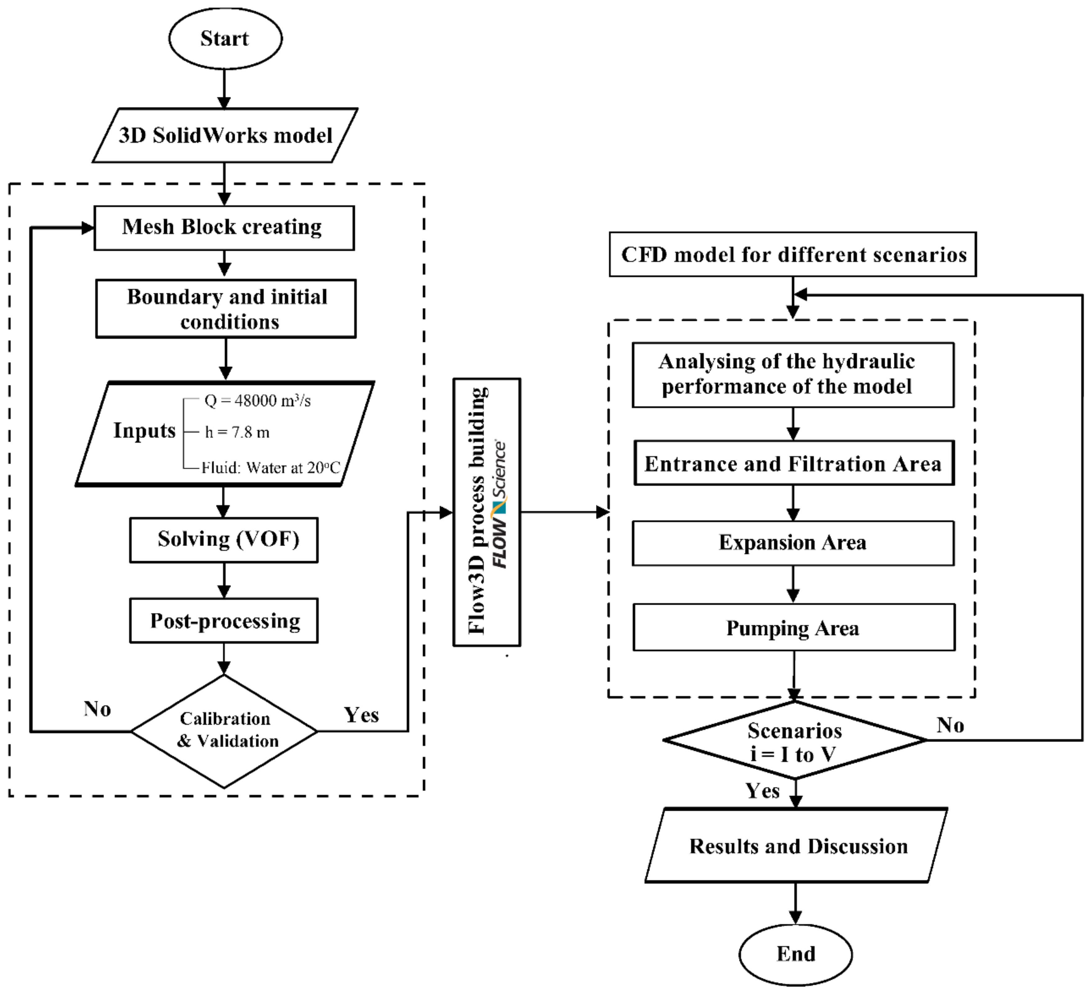
The flowchart of the research methodology that was used to achieve the study’s aims is shown in Figure 2.

The main advantages and reasons for using Flow3D to simulate the hydraulic flow conditions in the seawater intake system of this study are as follows:

Accuracy:

Using our industry-leading TruVOF algorithm, FLOW-3D produces high-accuracy simulation results faster. Since its debut 35 years ago, TruVOF, a pioneering volume of fluid tracking technology, has continued to set the industry standard for flow accuracy. FLOW-3D is the result of years of collaboration with the world’s finest scientific, manufacturing, and research firms to produce realistic simulations and a collaborative workflow.

Efficiency:

FLOW-3D uses the FAVOR™ meshing approach, which significantly improves the issue setup by incorporating geometry directly into the mesh, allowing for rapid parametric tweaks without the time-consuming re-meshing required by other computational fluid dynamics tools [36,37]. Engineers spend their efforts visualizing, optimizing, and working on design concepts that have shorter runtimes and higher accuracy.

High Performance Computing:

To meet the industry’s most demanding simulations, FLOW-3D smoothly transitions from desktop workstation solutions to high-performance on-demand cloud computing and cluster solutions.

While developing the appropriate model, the user will navigate through five primary tabs. These are the tabs:

• Navigator: The user will see the simulation files, portfolio overview, and the path to the simulation files’ locations on this screen.
• Model Setup: The flow domain has been designed, meshing has been completed, and physical and numerical parameters have been entered. The model setup tab has six sub tabs.

  ▪

  General: This sub tab determines the simulation’s completion duration, fluid compressibility, kind of interface, type of units, quantity of fluids, and degree of precision.

  ▪

  Physics: Fluid source, air entrainment, sediment, gravity, cavitation, viscosity and turbulence, heat transmission, and moving objects are only some of the physical possibilities available depending on the situation.

  ▪

  Fluids: This sub-tab allows you to select the working fluid and its parameters.

  ▪

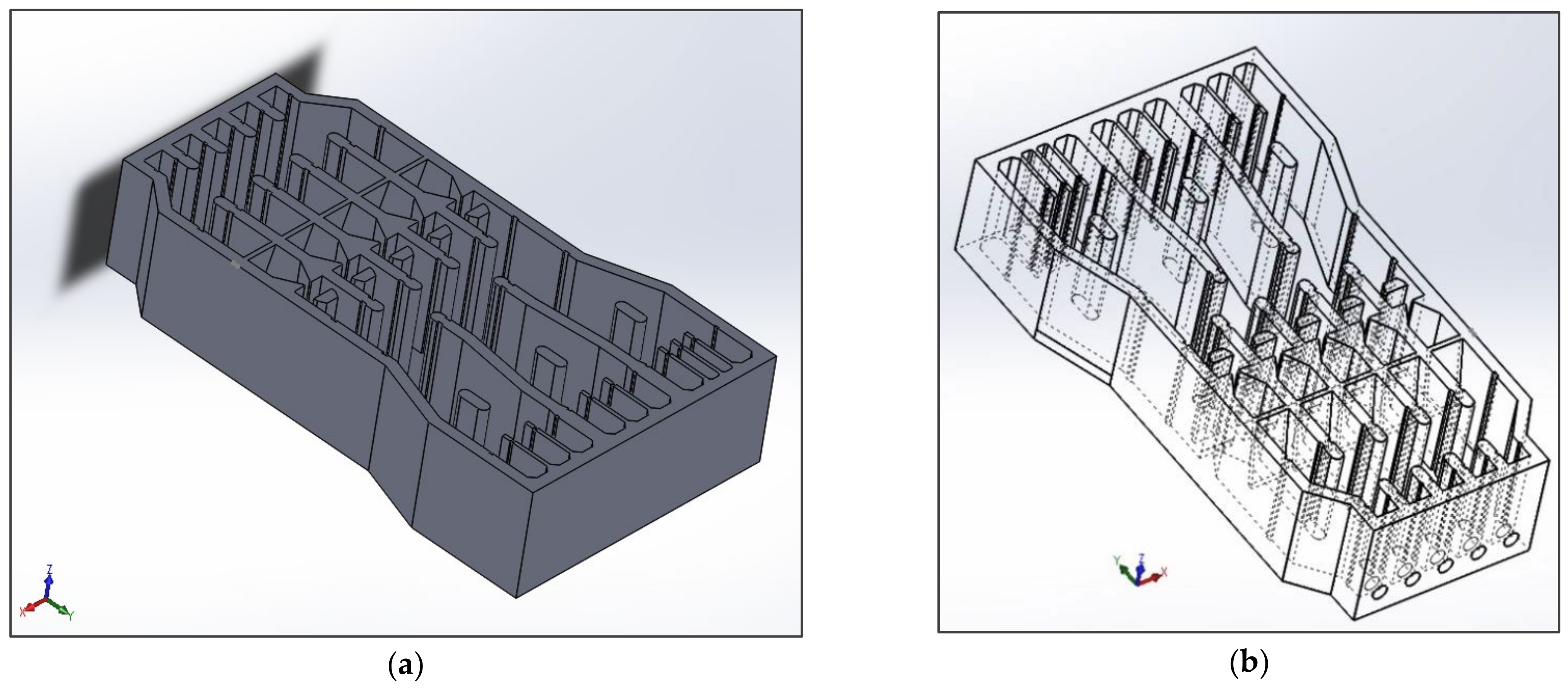
  Meshing and Geometry: This sub-tab is where you construct the domain’s geometry, as well as the beginning and boundary conditions. The user can either use the software’s drawing features or import an STL-formatted executable drawing file. The user can construct a primitive mesh that fits the geometry with Flow-3D (see Figure 3).

  ▪

  Output: Here, the desired intervals and data types are determined. The restart data interval specifies how frequently the data will be saved in the event of a restart. While analyzing the answers, the selected data interval determines the size of the timeline steps.

  ▪

  Numeric: Convergence controls, stability factors, viscous and/or turbulence stress and pressure solver options, momentum advection, and fluid flow solver options are all found under this sub tab.

• Simulation: This screen displays information about the simulation’s progress. When needed, you can look at graphics connected to the simulations, such as pressure iteration count, time step size, etc.
• Analyze: The user can basically study the results as a text or in 1D, 2D, and 3D charts using this table. The ISO surface and color variables are chosen from a list of alternatives based on the study’s goal. To analyze, any time interval and any part of the system can be chosen.
• Display: This is the screen where the user can examine the visual results of the analyze tab’s criteria. It is possible to take a screenshot of the screen or create a movie.

2.1. The 3D Modeling of the Basin

To capture these vortices, eddies, and related effects, there is a need for three dimensional CFD software. In all scenarios, flow simulation for the seawater intake system of this study was undertaken completely in 3D. Since the 2D model differs from the prototype in the following cases:

• In the 2D model each pump was modeled as a circle and flow sucked from the circle border. However, in the prototype condition the suction of the pump is located in an elevation below the water level.
• In the 2D model the effect of the bottom is not considered. Under low velocity conditions this does not have a considerable effect on the result of the model.

Therefore, to obtain assurance about the obtained results, all scenarios are modeled as three-dimensional, which are presented in the following section:

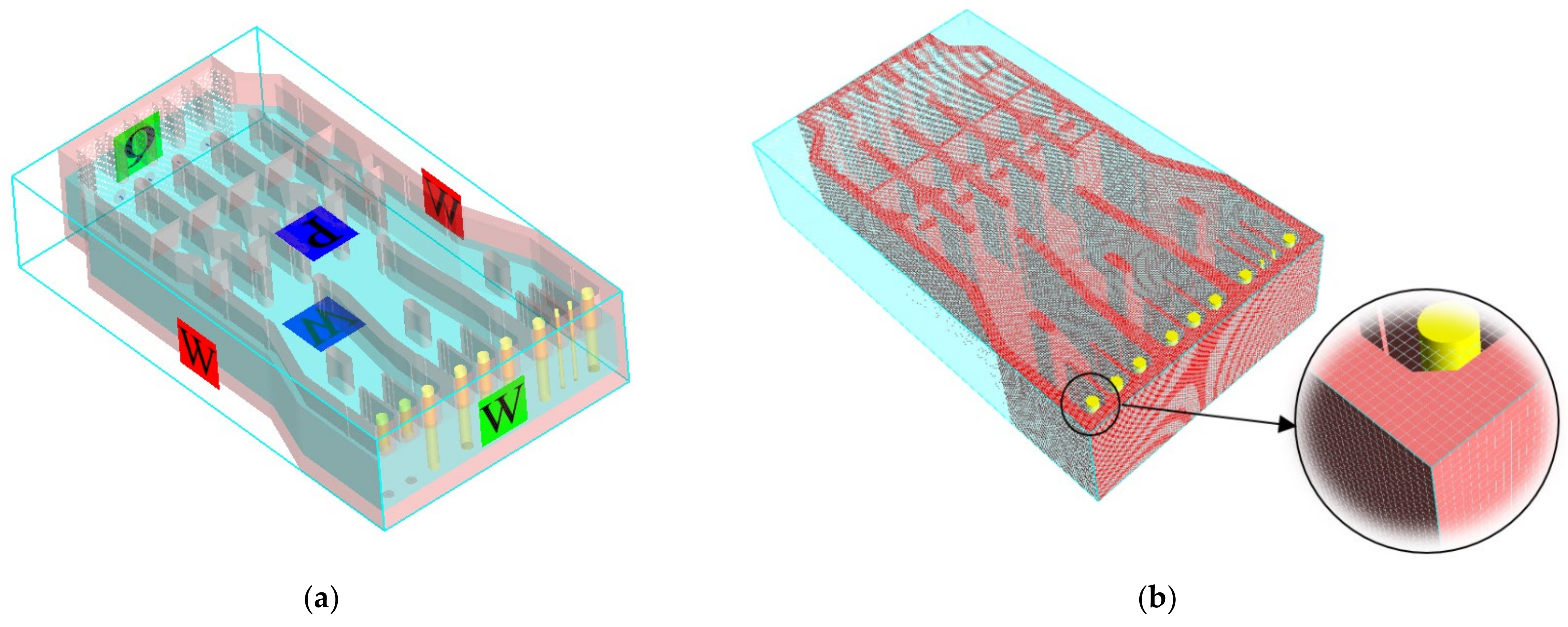
Boundary conditions should be appropriately defined. Based on the flow characteristics, the specific pressure at the top of the seawater intake was set to atmospheric pressure. The entrance area of the inlet pipe cross section was set at a flow rate (Q). The far end of the basin outlet pump was defined as an outflow, and the remaining boundaries and the flow domain envelope were defined as a wall (W) with a roughness height of 2.0 mm. The authors selected this value because it is similar to medium-roughness concrete channels (Figure 4a).

The FLOW-3D mesh generation technique employs a structured, rectangular, and Cartesian mesh that is independent of the geometry being used, providing the user with convenience and flexibility. The size of the cell used is 250 mm, and the simulation is run with a mesh block (each cell was 250 mm in the X-, Y-, and Z-axes). The block mesh contained 401,158 cells (Figure 4b).

When the basin is operating normally, one pump from each group of pumps is standing by. This spare can be changed between pumps. Another situation is the maintenance period of screens. Thus, the 3D model of the basin is solved for five different scenarios:

• Scenario I: Normal condition. (All screens are operational and from each group of pumps, one is on standby. Furthermore, in the entrance area, the right polyethylene pipe is on standby).
• Scenario II: Normal condition. (All screens are operational and from each group of pumps, one is on standby. Furthermore, in the entrance area, the left polyethylene pipe is on standby).
• Scenario III: Normal operation by changing the spare pump. (All screens are operational and from each group of pumps, one is on standby. Furthermore, in the entrance area, the middle polyethylene pipe is on standby)
• Scenario IV: Normal condition + Firefighting pump. (All screens are operational and from each group of pumps, one is on standby. Furthermore, in the entrance area, the left polyethylene pipe is on standby).
• Scenario V: One screening system is in the maintenance period.

2.2. Validation and Accuracy

At its core, a CFD program solves a set of equations subject to the specified initial and boundary conditions. Every equation that is solved describes the typical behavior of a physical phenomenon within some range of validity. The accuracy of an equation and the associated range of validity are limited by many factors, including:

• The accuracy and precision of the experimental/analytical measurements that were used to develop the equation;
• The assumptions used to develop the equation;
• The understanding of the phenomena described by the equation;
• The accuracy of the empirical constants used in the equation.

In general, equations describing quantities that are resolved by the mesh (e.g., heat transfer, surface tension, etc.) are more accurate and have a wider range of validity than those compensating for the finite resolution of the solution (e.g., turbulence models, air entrainment, etc.) since the latter must rely on empiricism or assumptions to compute a solution [38]. In either case, it is important to accept that the solution will only be as accurate as the equations and to account for this error when interpreting the results. Accordingly, in the present study, the accuracy of numerical modeling was evaluated based on two approaches. In the first approach, the accuracy of the values of hydrodynamic parameters including average velocities ($V$), flow depth ($h$), and discharge ($Q$) are compared with the values obtained from the analytical solution. The relative error values of the following equation are used:

$$Error \%=100\times \frac{X_{Analytical}-X_{Numerical}}{X_{Analytical}}$$

(5)

where $X_{Analytical}$ is the actual value of the parameter (analytical values) and $X_{Numerical}$ is the simulated value of the parameter. As displayed in

Table 1. Comparison of validation and accuracy results and numerical model calibration for hydrodynamic parameters.

Hydrodynamic Parameters	$\mathit{V} \left(\mathit{m}/\mathit{s}\right)$	$\mathit{h}\left(\mathit{m}\right)$	$\mathit{Q} \left({\mathit{m}}^3/\mathit{h}\right)$
Analytical solutions	0.23	7.8	48,000
Numerical modeling	0.21	7.17	46,691
Error %	8.69	8.07	2.72

, the simulation of the hydrodynamic parameters including average velocities ($V$), flow depth ($h$), and discharge ($Q$) of the simulated flow is close to the analytical solutions. Based on the findings of numerical modeling, the maximum relative error of the numerical model in the parameters of average velocities is equal to 8.69%. Additionally, the maximum error of simulating the flow depth ($h$) compared to the analytical solutions state is calculated to be 5.8%.

In the second approach, the accuracy and sensitivity of numerical modeling to the size of selected cells in the numerical model are investigated. In the present study, a mesh sensitivity analysis was conducted with five different cell sizes.

Table 2. Mesh accuracy and sensitivity analysis.

	Type of Mesh
Parameters	Cell Size 20% Smaller	Cell Size 10% Smaller	Main (Selected for all Simulations)	Cell Size 10% Larger	Cell Size 20% Larger
No. Cells	482,651	442,785	401,158	362,713	327,012
Velocity (m/s)	0.221	0.224	0.23	0.237	0.249
Analytical velocity (m/s)	0.21	0.21	0.21	0.21	0.21
Error (%)	4.97	6.25	8.69	11.4	15.66

shows the results of the mesh sensitivity analysis on the velocity in the reference area for all operational screens and from each group of pumps, one is on standby. As can be seen, if the cell size is smaller than the main mesh, it does not affect the accuracy of the simulation and if the cell size is larger than the main mesh, the error can increase about twice.

Examining the accuracy of numerical modeling with these two approaches shows that the implemented numerical model has acceptable accuracy. Therefore, the hydraulic performance of the flow for the seawater intake can be evaluated in different operating scenarios.

3. Results and Discussion

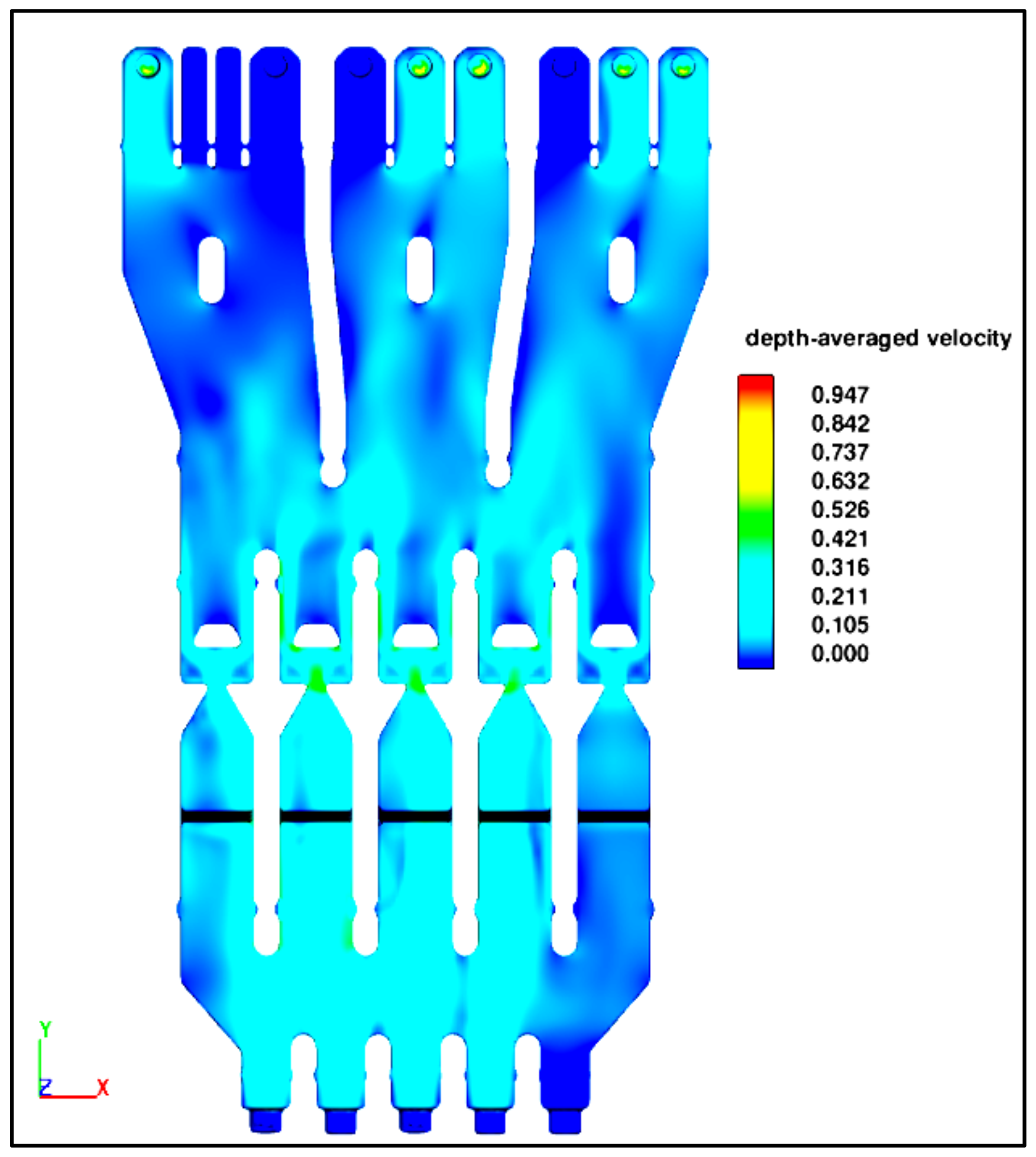
3.1. Scenario I

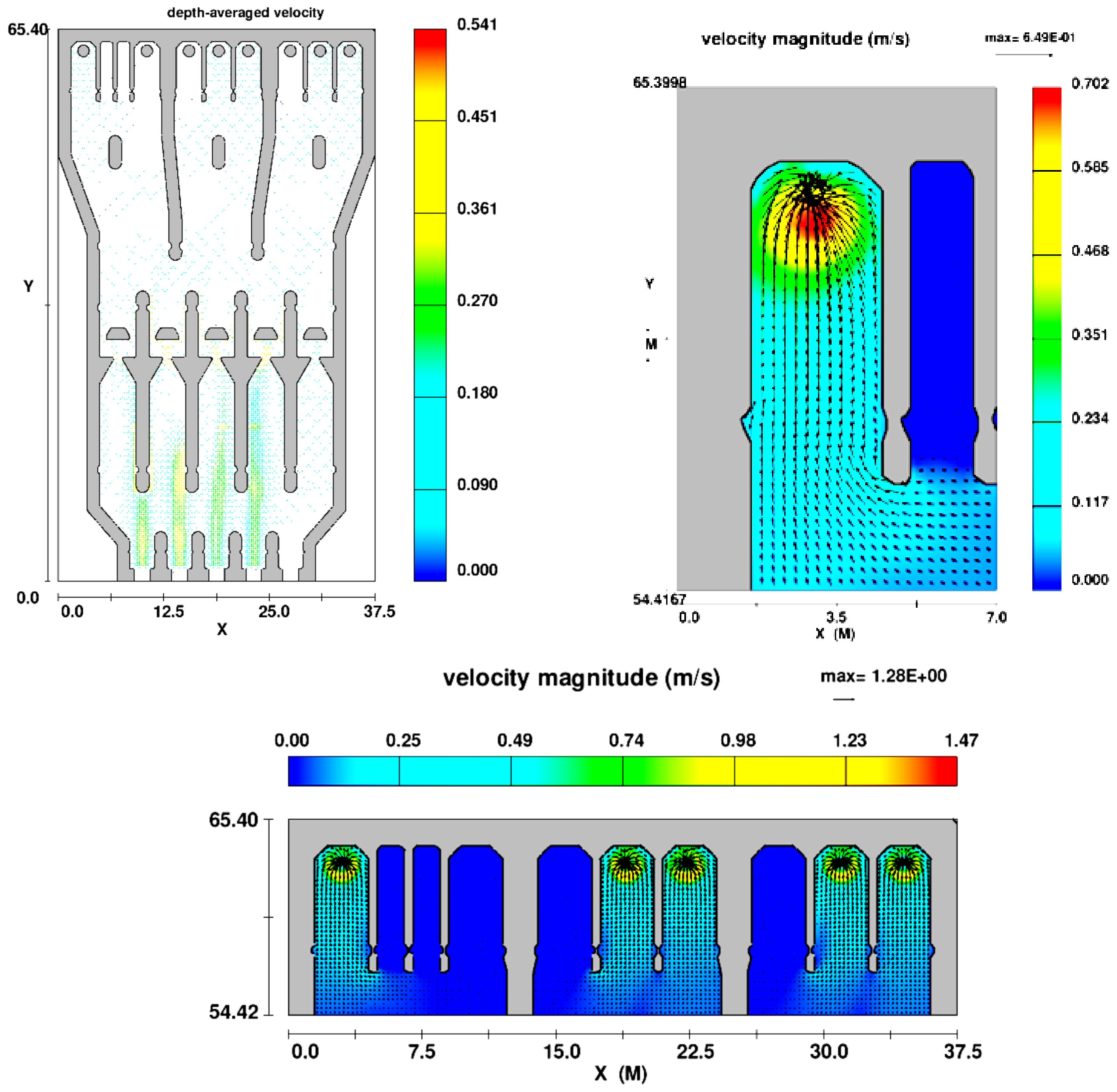
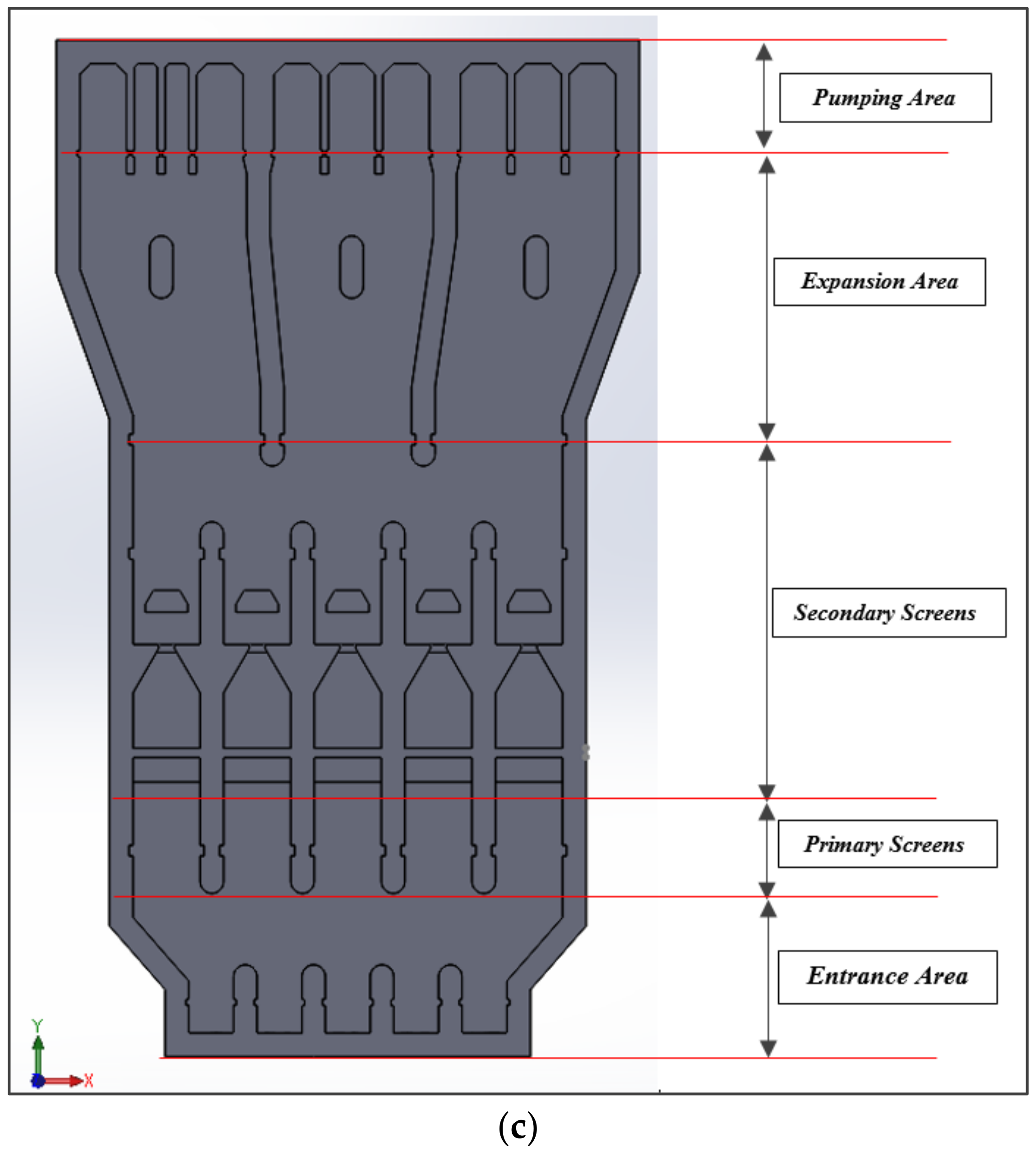
In this scenario, all screens are operational and one pump from each pump group is on standby. Figure 5 and Figure 6 show the velocity contours and the velocity vector field for the basin in this scenario. In the entrance area, the basin walls diverge and the flow pattern does not follow the wall direction completely and some small local vortexes may happen. The channels of the filtration system are located after the entrance area. The primary filtration system (bar screens) is not sensitive to the effects of turbulence and causes the flow to be laminar. Regarding operation conditions, velocity before this filter should be less than 0.3 m/s. Model observations show that the long distance between the entrance and the primary filtration system, as well as the narrow filtration channels, causes the flow to become parallel before entering the bar screens. This results in vortex creation being an impossibility. The straight flow of jets from the outlet polyethylene pipes increases the local velocity in the primary filtration system (bar screen). Therefore, as seen in the figures, the local velocity in the primary filtration system is slightly greater than 0.3 m/s. In order to reduce the flow velocity in this area, it is recommended that the entrance area is extended. An increase in the distance between these two areas will provide conditions for energy dissipations. Consequently, there will be a reduction in the flow velocity before the primary filtration system.

The area after the filtration system and before the pumping section is important in the hydraulic point of view. Because:

• Flow velocity at the exit of secondary filtration system is considerably high.
• The angle of expansion after the filtration system is high.
• The width of each bay is large.

The type of secondary filtration system causes high local velocity. Two solutions are available to reduce the effect of this high velocity on pump operation:

• Increasing the distance between filtration system area and pumping section.
• Usage of flow distribution blockage or baffles.

In this case, the distance between the pumping area and the filtration system is large. Therefore, the impact of the high fluid velocity at the outlet of the filtration system on the pumping area is low. Some local swirls after the support of filters might be created and dissipated after a few meters.

As expected, the flow direction does not follow the direction of the walls at the beginning of the expansion area, causing local swirls beside the walls. This local vortex has a low velocity and has no effect on the pumping system during operation.

After the expansion area, there is an area in which the fluid flow enters at an incline to the lateral wall of the pumping bay. A guide wall is introduced to reduce the possibility of vortex creation. Furthermore, the distance between the pump installation area and the end of the expansion wall is considered large to be able to quell the effects of angular flow. As a result, the flow pattern is approximately parallel to the later wall of the pumping bay. Thus, the inclination of the flow is negligible. Overall, for hydraulic flow conditions in this scenario, there is no possibility of rotating flow or vortex formation in the pumping area and the correct orientation of the pumping area is achieved.

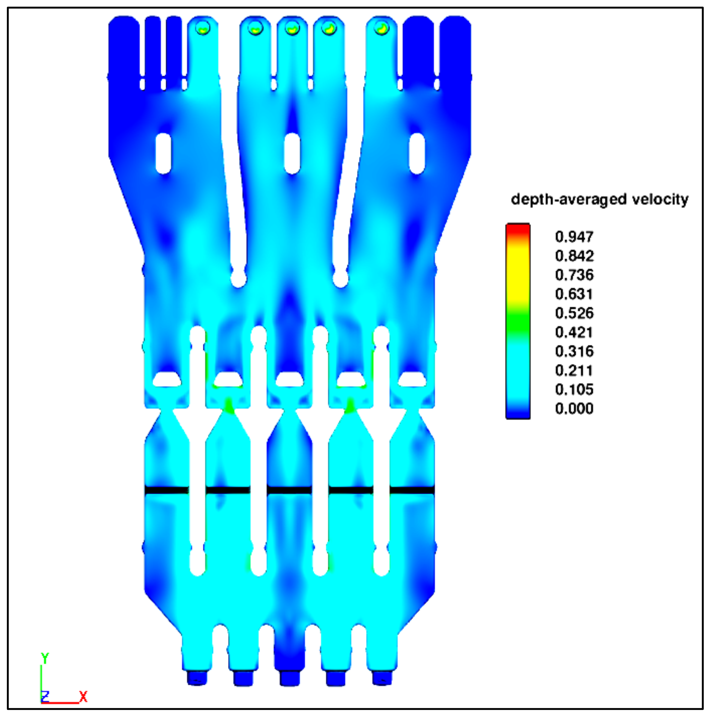
3.2. Scenario II

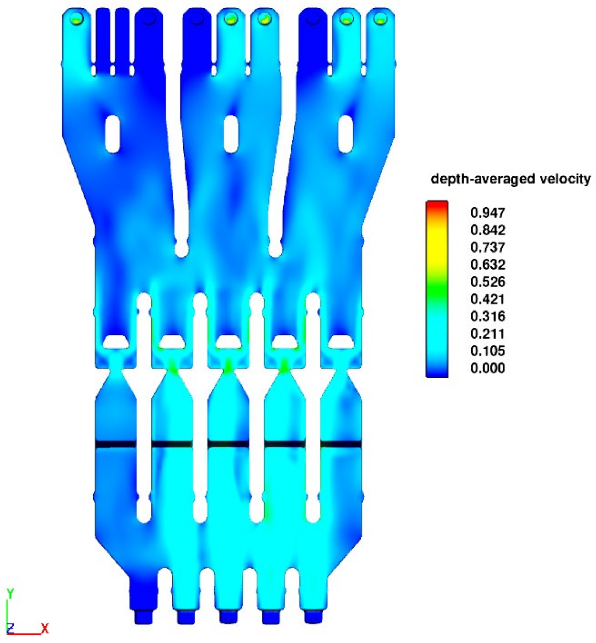
In this scenario spare submarine pipelines are selected in such a way that differs from the previous scenario. Figure 7 and Figure 8 show the velocity contours and field vector of velocity at the basin in scenario II. It is obvious that there is no difference in the flow pattern when compared with the first scenario. The study shows that there is a small shift in the flow pattern near the filtrations area. However, generally, flow pattern does not change. It should be considered that the suitable velocity for the bay suction sump of each pump is about 0.3–0.5 m/s. In this basin, the average velocity before the pump pit is about 0.05–0.07 m/s and in each pump pit it is 0.11–0.15 m/s. Due to the fact that the main flow velocity in the basin is small, changing the location of the inlet pipe will not change the hydraulic conditions of the flow. In other words, due to the appropriate length of the basin and the sidewalls, the flow pattern similar to the previous scenario is maintained.

3.3. Scenario III

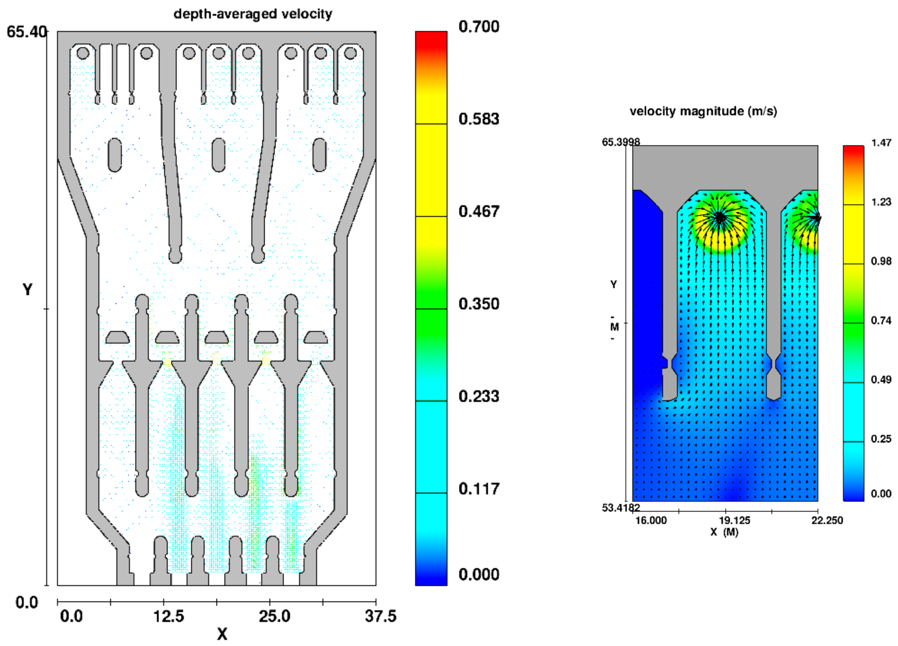
In this scenario, spare submarine pipelines and spare pumps are selected in such a way that differs from the two previous scenarios (scenario I, scenario II). In this scenario, the middle submarine pipeline is considered as a spare and five intermediate pumps are running. Figure 9 and Figure 10 show the velocity contours and field vector of velocity at the basin in scenario III. In this scenario, the hydrodynamic performance of the intake basin is similar to that of previous scenarios. In the entrance area, as in previous scenarios, there is no intense turbulent flow and no special swirl and vortex were formed. In the filtration area, the flow passes at an average flow velocity of 0.25 m/s from the primary and secondary filters. In this scenario, the maximum flow velocity to the filtration area is slightly greater than 0.3 m/s. In order to reduce the flow velocity in this area, it is recommended that the entrance area is extended.

In the expansion area, the main flow is formed between the dividing walls, which increased the flow velocity compared to the previous scenarios in this area. The average flow velocity in the expansion area is 0.12 m/s and the vortex and swirls flow are not formed. In the area of the pumps, there is also a very laminar and stable flow, and the average flow velocity of the inlet to the bay for one of the pumps is about 0.15 m/s. Overall, for hydraulic flow conditions in this scenario, rotating flow or vortex in the pumping area are not formed and the proper operation of the pumping area is approved.

3.4. Scenario IV

In scenario IV, all screens are operational, and from each group of pumps, one is on standby. Furthermore, in the entrance area, the right polyethylene pipe is on standby. The only difference between the fourth scenario (IV) and the first scenario (I) is that the firefighting pumps are operational. Figure 11 and Figure 12 show the velocity contours and field vector of velocity at the basin in scenario IV. It is obvious that the flow pattern in this situation against the first scenario has no affective change. Considering that the capacity of the firefighting pumps is much lower compared to other pumps, their use will not have an adverse effect on the hydraulic condition of the pond. It should be noted that due to the suction of firefighting pumps in these bays, the flow of swirls or vortices flow is not formed.

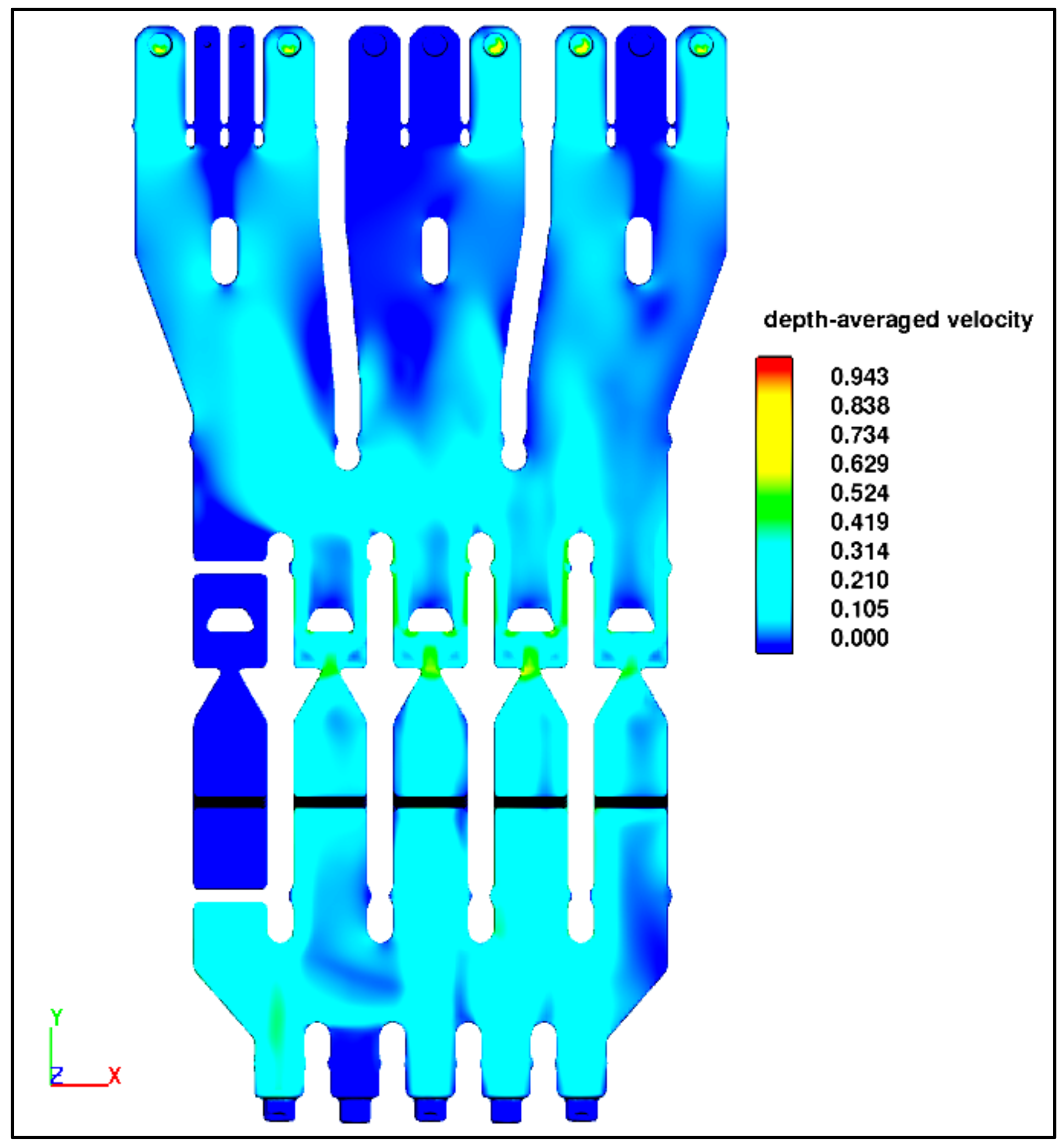
3.5. Scenario V: One Filter on Maintenance

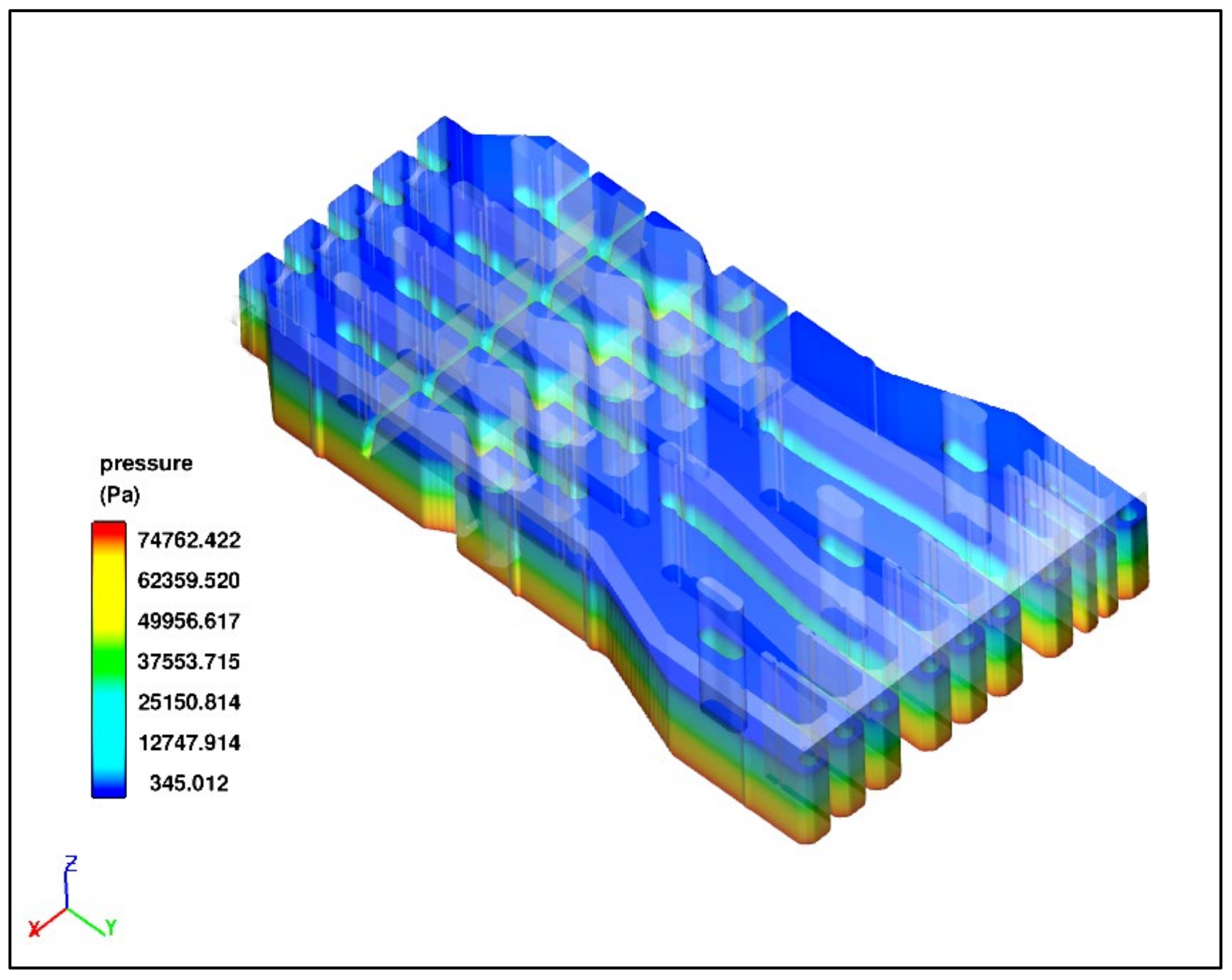
In this scenario, the model is solved for a situation that one of the five parallel filtration systems is on maintenance and so the related stop logs are closed. In this scenario, it is necessary that water transfers from the four remaining filters to each of the five bays. Figure 13 and Figure 14 show the velocity contours and field vector of velocity at the basin for scenario III. Figure 15 also shows contours of pressure.

Generally, the flow pattern near the pumps in this scenario does not differ from previous scenarios. This means that the design of the flow distribution area is acceptable and the system can work with four screens continuously.

Figure 12 shows the pressure contours for this scenario. Pressure contours for other scenarios are the same. Although, the distribution pressure in this scenario is more than other mentioned scenarios. Most of this loss happens in the secondary screen system when the flow is passing from the narrow entrance to the exit of the dual flow band screens. In 3D modeling, increasing the depth increases pressure values and is calculated from equation P = gH.

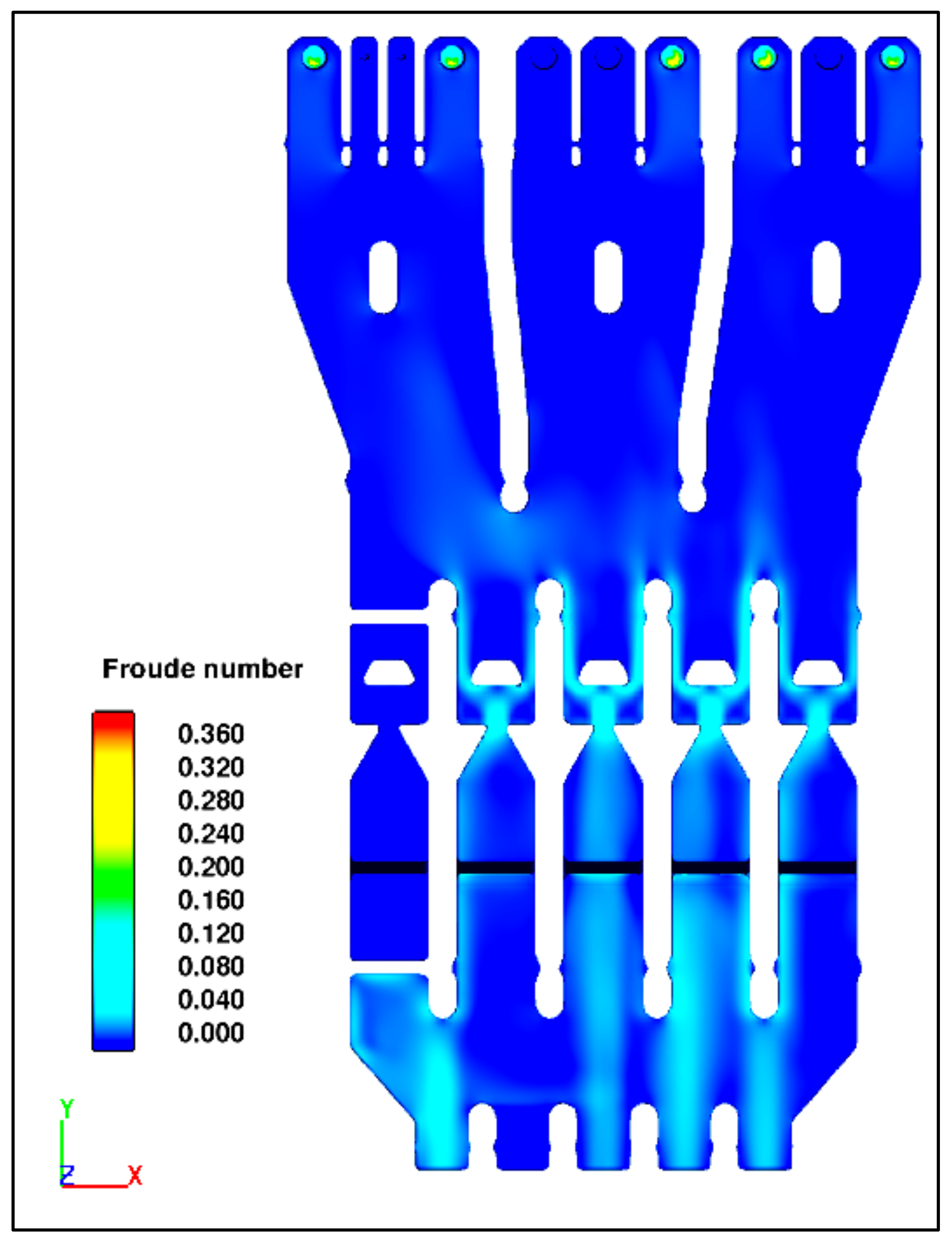
In Figure 16, the contours of the Froude number of the flow are extracted from the numerical model, which shows that the whole flow field is subcritical. For subcritical flow, the depth is greater and the velocity lower, so the Froude number is always less than 1.0. According to Figure 16, the Froude number in the entrance area is variable due to the higher velocity of the outflow from the pipes and is greater than in other intake areas. However, the Froude number is still less than 1 and the flow is subcritical. By passing the flow through the filtration areas, the velocity will decrease, the flow pattern will become more regular, and this process will be completed by reaching the expansion area. In other words, the filtration and expansion areas will help to stabilize the flow pattern and keep good flow conditions in the pump area as a completely subcritical flow.

Hydraulic loss is a measure of the reduction in the total head (sum of elevation head, velocity head, and pressure head) of the fluid as it moves through a fluid system. Hydraulic loss is unavoidable in real fluids. It is present because of: the friction between the fluid and the walls of the basin; the friction between adjacent fluid particles as they move relative to one another; and the turbulence caused whenever the flow is redirected or affected in any way by components such as entrances and screens, pumps, expansion, flow reducers, and fittings. The hydraulic loss for flow in a seawater intake can be expressed in terms similar to that for an enclosed open channel, using the hydraulic radius and the length of the basin. The hydraulic loss ($h$) may be calculated in Equation (6):

$$h=f\frac{L}{R_h} \frac{V^2}{2g}$$

(6)

where f: Darcy friction factor; L: length of channel (m); R_h: hydraulic radius; V: average velocity (m/s); and g: gravity (m/s²). The hydraulic losses that occur in a seawater intake basin are sometimes called minor losses [39]. For all minor losses in turbulent flow, the head loss varies as the square of the velocity. Due to the fact that the velocity values in the basin are small, the hydraulic loss in such basins can be ignored.

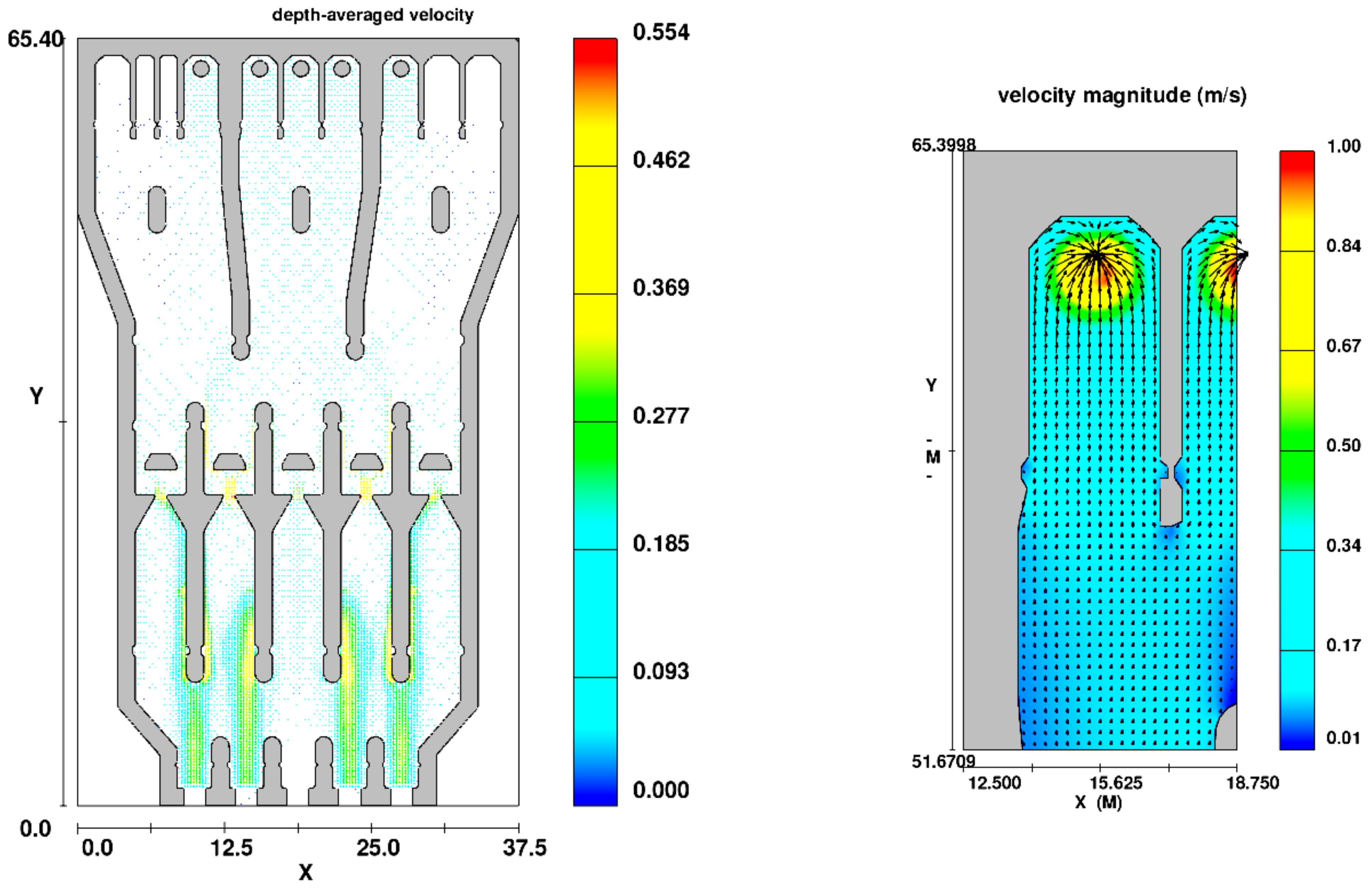
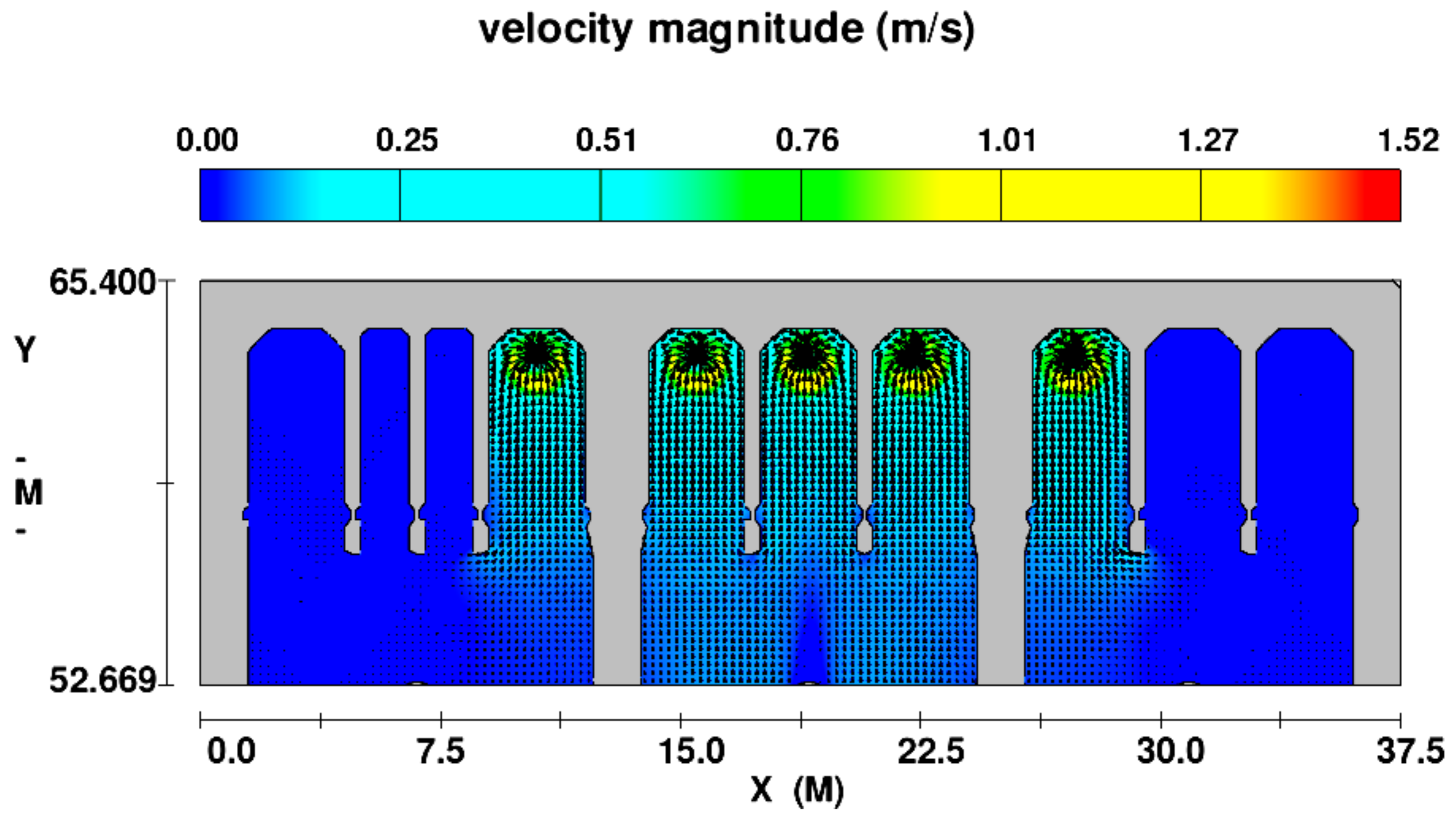
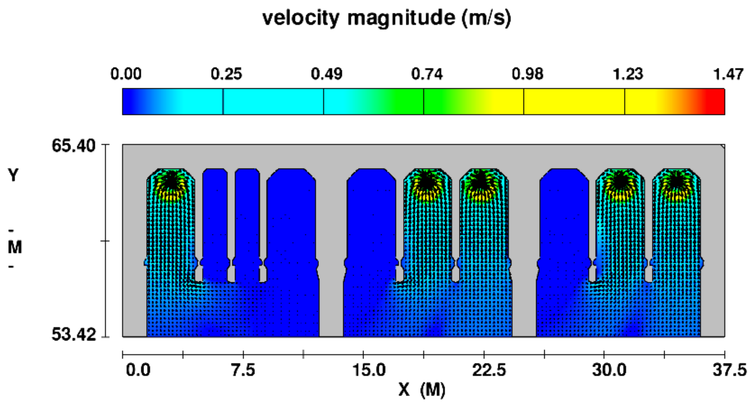
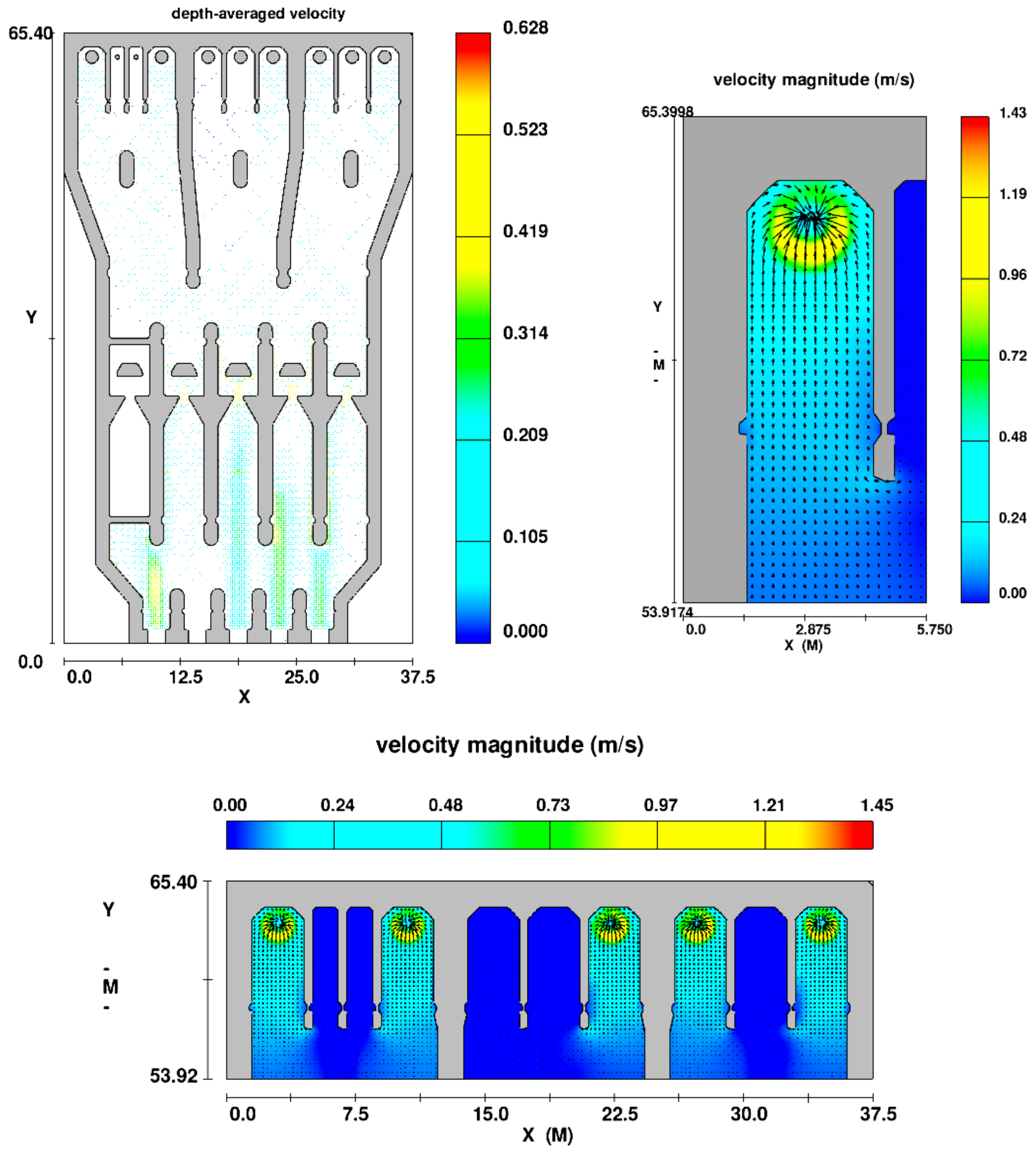
3.6. The Flow Pattern near the Pump Suction

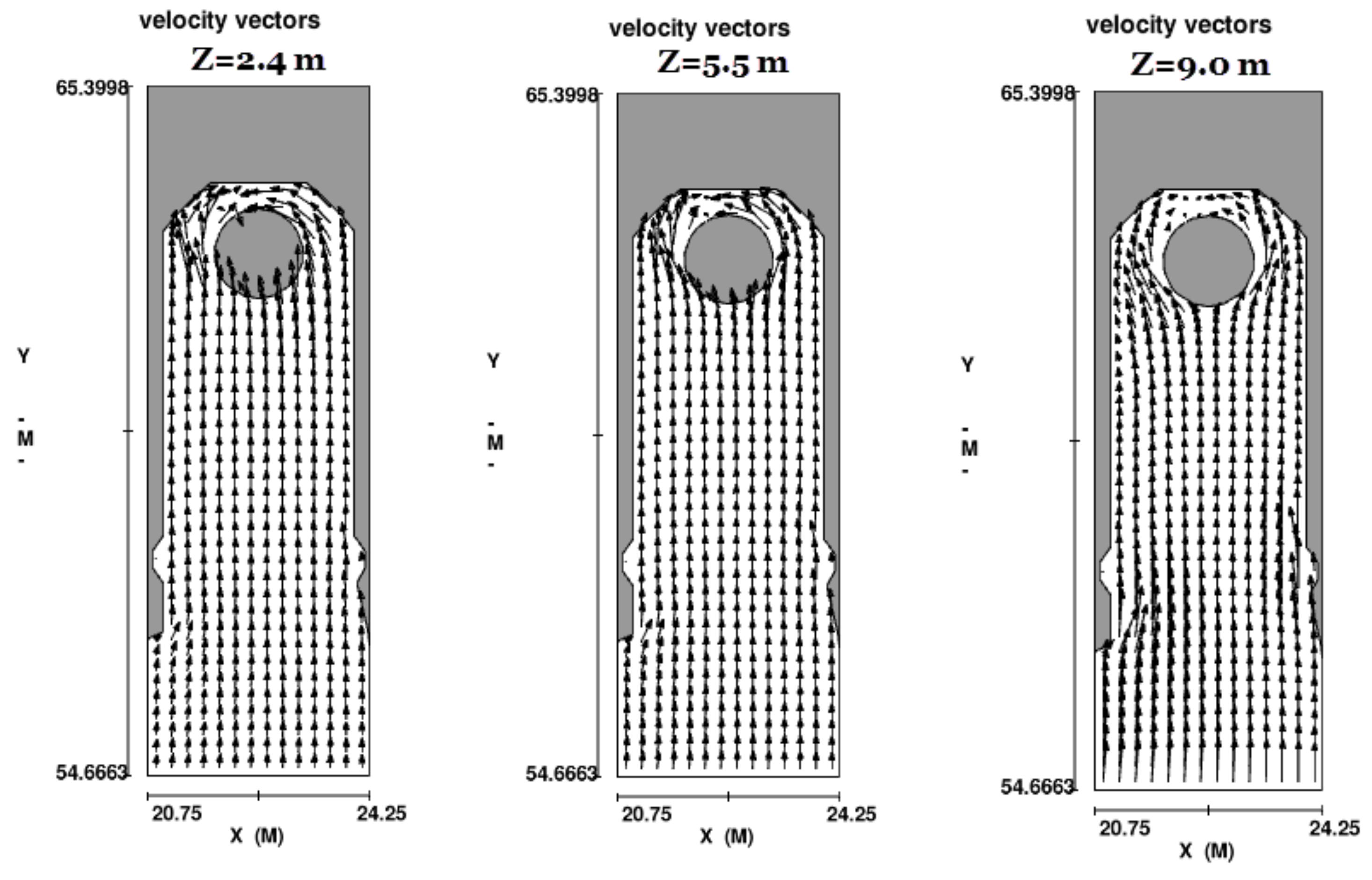
Figure 17 shows the vector field of velocity in a vertical section near a pump. It depicts the flow from the surface to the bottom of the pump suction. Therefore, flow is completely 3D in this situation.

Vortexes form between the pump suction and intake tank fluid surface. Surface vortices may be reduced with increasing depth of submergence of the pump bells. However, there are also situations where increasing depth has negligible effects or even increases surface vortex formation due to stagnant and therefore unstable liquid. Surface vortices are also highly dependent on approach flow patterns and the stability of these patterns, as well as on the inlet Froude number. The above situation complicates the establishment of a minimum depth of submergence as a definitive measure against vortices. To achieve a higher degree of certainty that objectionable surface vortices do not form, modifications can be made to intake structures to allow operation at practical depths of submergence. 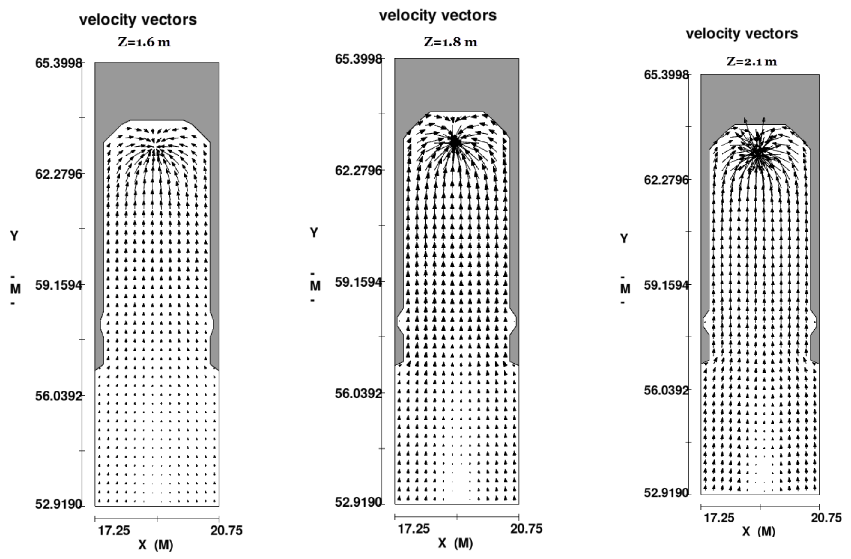Figure 18 shows the velocity vector field around this pump at different elevations. Therefore, it can be said that in the prototype case, no vortex is created around the pumps.

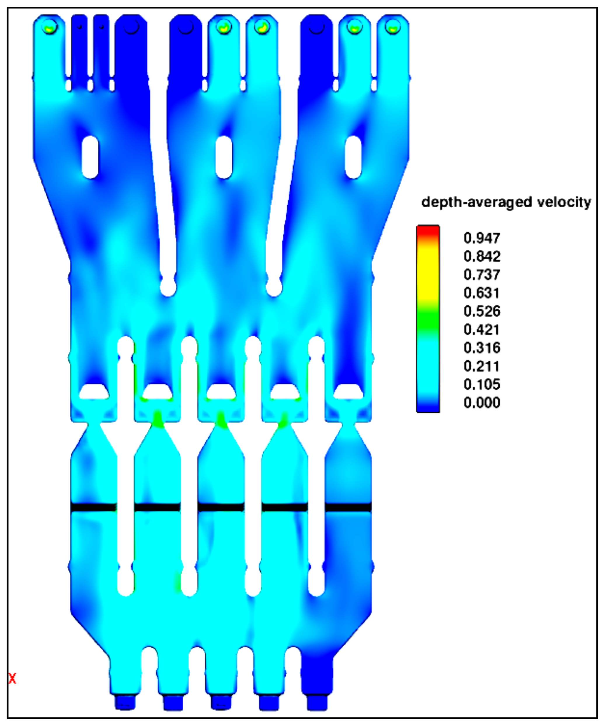
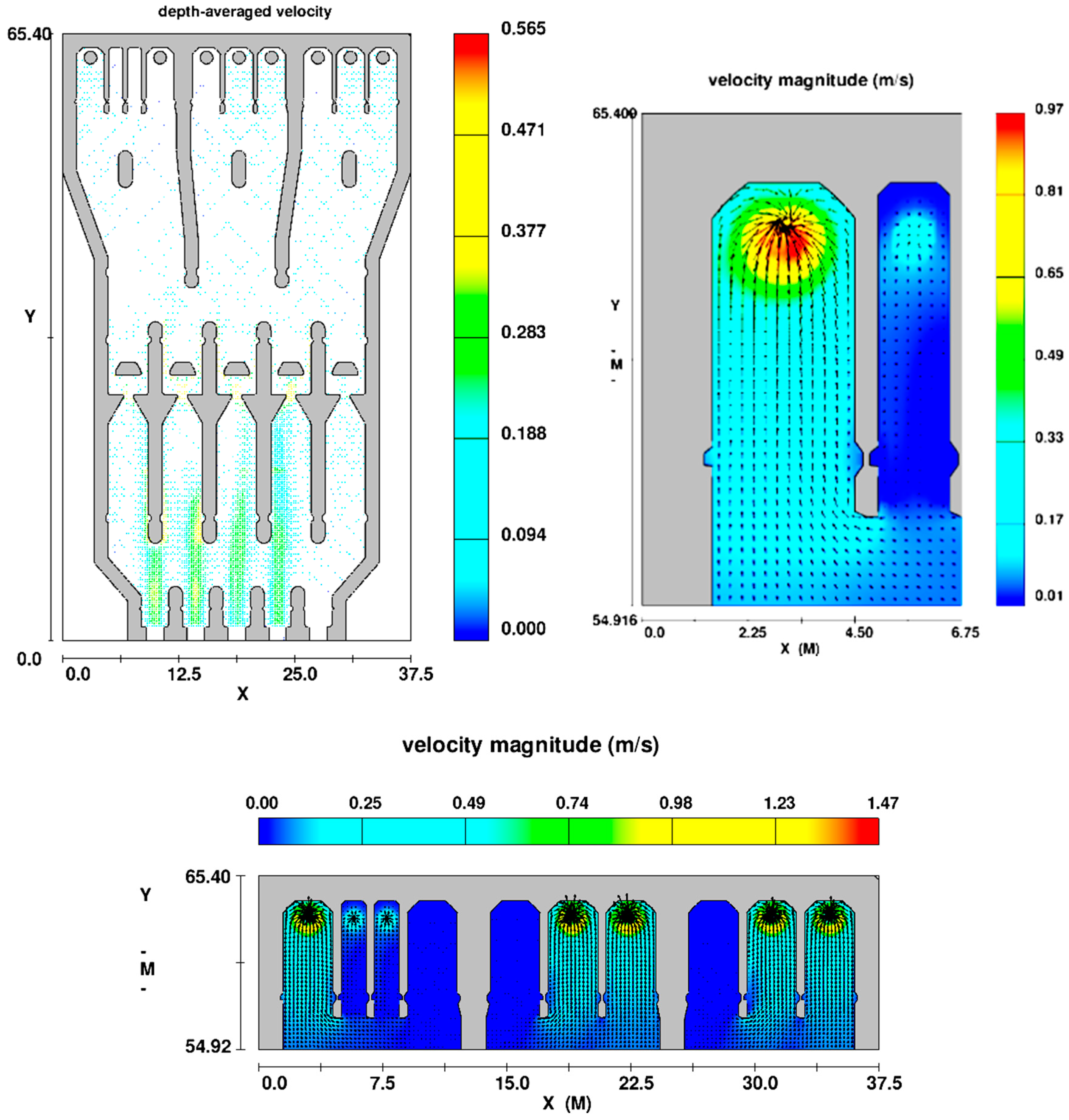
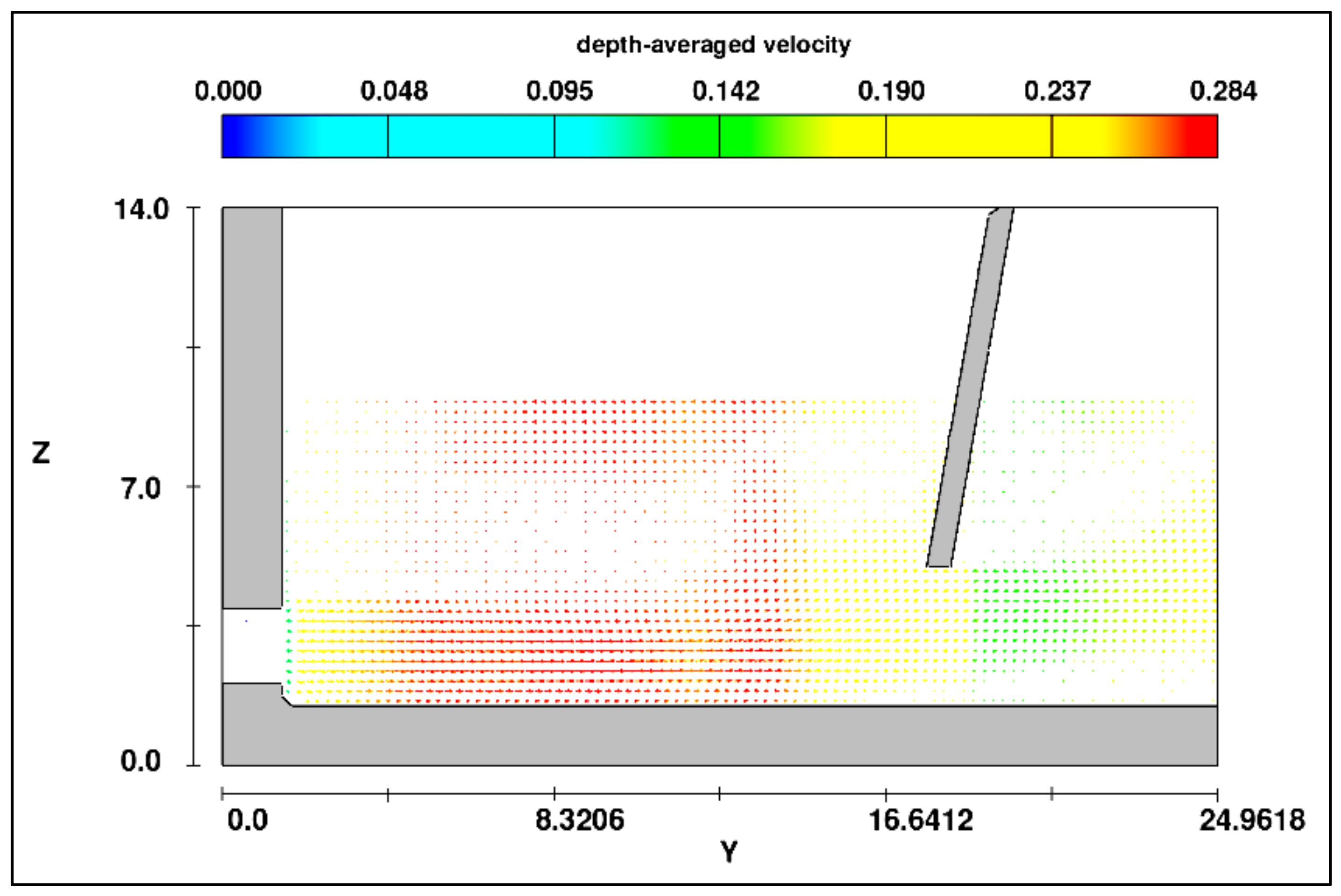
3.7. The Flow at the Entrance Area of Basin

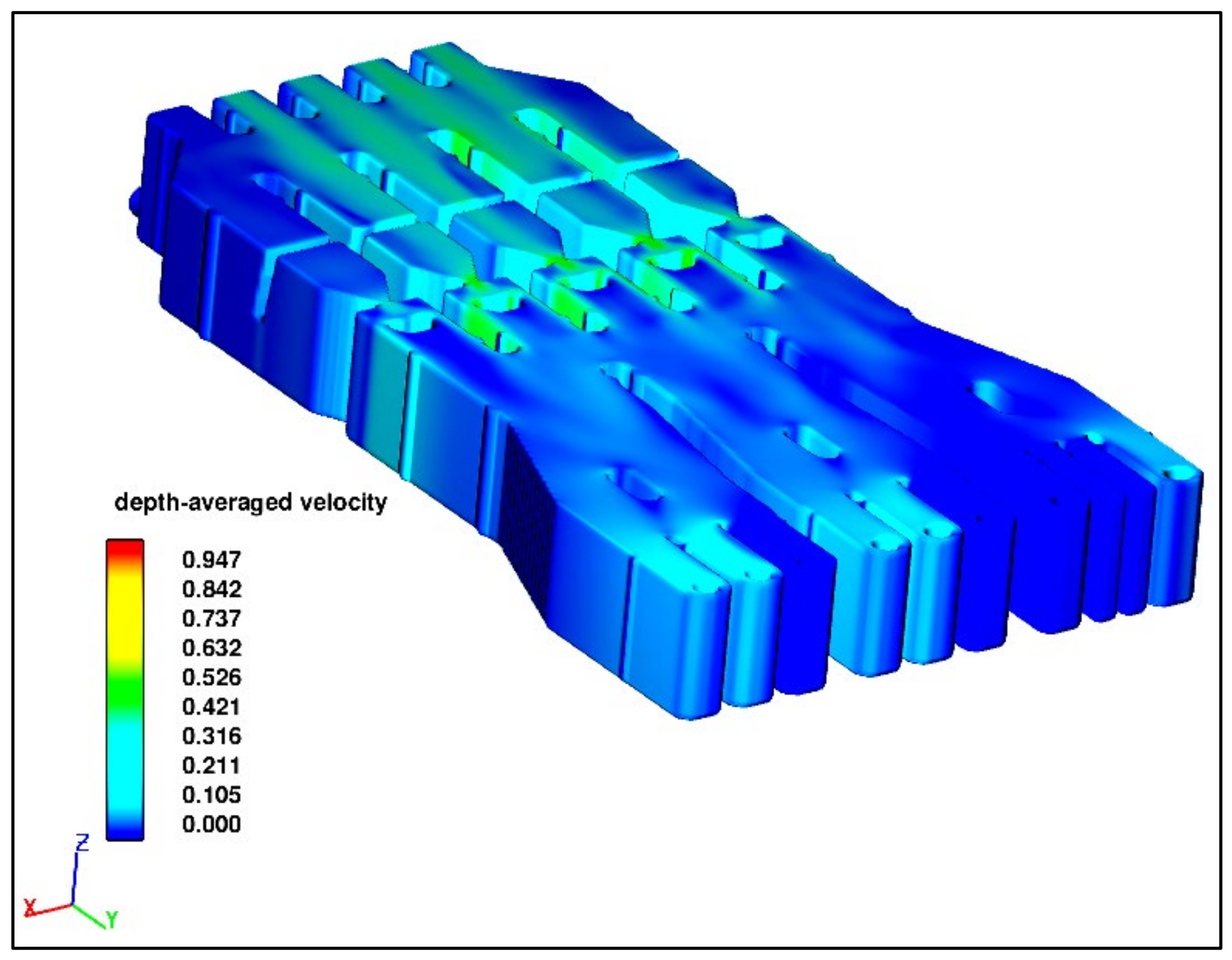
In the entrance area, the geometric changes in the basin are greater than other areas and the hydraulic parameters in this area should also be considered. There are five rectangular conduction channels, also called filtration channels, in the entrance area. This rapid change in geometry can cause some vortex in the entrance area. Figure 19 shows the flow pattern in a vertical section that passes through the center of one of the entering pipes. A reverse of flow nearby the surface in a small region is shown. This reverse flow dissipates after a distance about 4 diameter of an inlet pipe (8 m). In Figure 20, the flow velocity contours are provided for three-dimensional seawater intake.

4. Conclusions

The efficiency and performance of pumping stations involving multiple pumping units depend not only on the efficiency of the pumping units but also on the flow patterns of the intake sump basin. The improvement in the pumping station flow pattern can effectively improve the operating performance of pumps, reduce sedimentation, improve the reliability and economy of the pumping station, reduce costs, and improve efficiency. Using numerical modeling, the hydraulic performance and flow pattern of pumps were checked under a variety of different operating conditions. The following are the conclusions derived from the study:

Entrance and Filtration Area: The structure and configuration of these areas of the basin and the flow pattern has a great impact on making the flow steadier and avoiding turbulence. The outflow from the polyethylene pipes increases the local velocity in the primary filtration system (bar screen). Results show that the local velocity in the primary filtration system is slightly greater than 0.3 m/s. A flow velocity greater than 0.3 m/s can increase turbulence and cross-flow in this area. In order to reduce the flow velocity in this area, it is recommended that the entrance area is extended. An increase in the distance between these two areas will provide conditions for energy dissipations, consequently, a reduction in the flow velocity before the primary filtration system.

Expansion Area: In all scenarios, the numerical model results show that maintaining a small angle of divergence of each wall from the influent conduit minimizes the difficulty in spreading the flow uniformly. Analysis the outputs of the CFD model shows that the installed flow distribution baffles dissipate the energy of the incoming flow from the before pumping area. In this area and in different scenarios of pump operation, the flow pattern when approaching the pumps will change in a divergent and uniform pattern.

Pumping Area: This study investigated several typical approach flow conditions for different combinations of pumps operating in a single intake structure. Numerical modeling results show that the presence of dividing walls between pumps prevents the formation of unfavorable hydraulic conditions in changing scenarios. However, adverse flow patterns can frequently occur if dividing walls are not used. To achieve a higher degree of certainty that objectionable surface vortices do not form, modifications can be made to intake structures to allow operation at practical depths of submergence.