
Effects of Sea Level Rise on Tidal Dynamics in Macrotidal Hangzhou Bay


Abstract
:1. Introduction
2. Methods
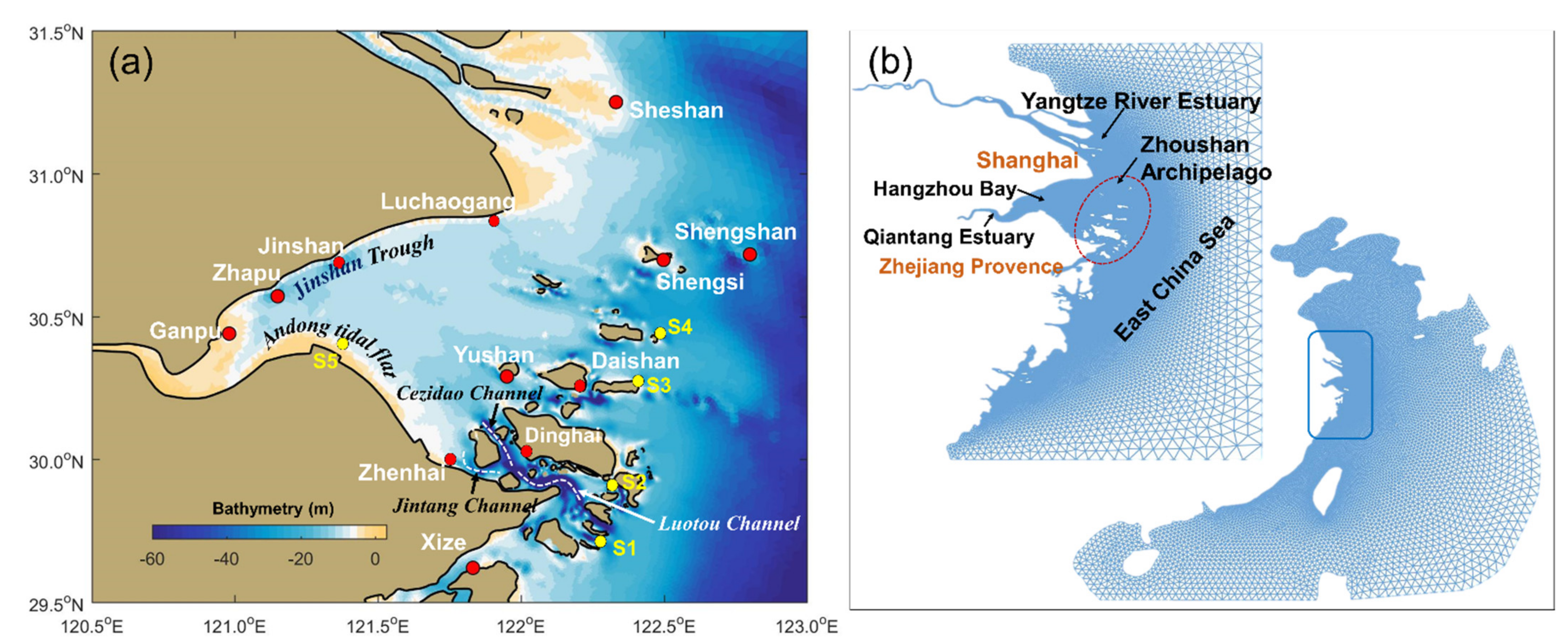
2.1. Study Area
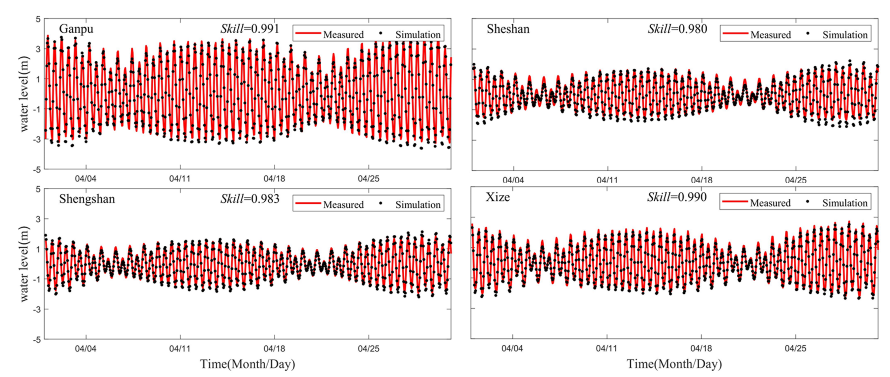
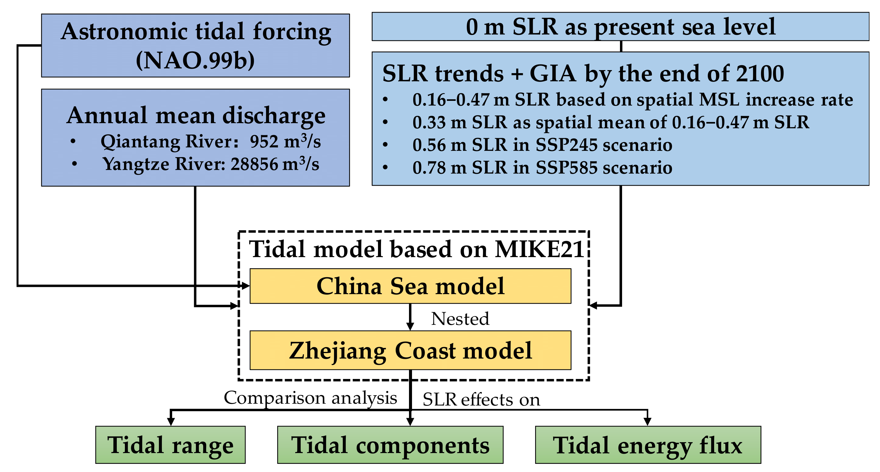
2.2. Model Configurations
2.3. SLR Trends
3. Results
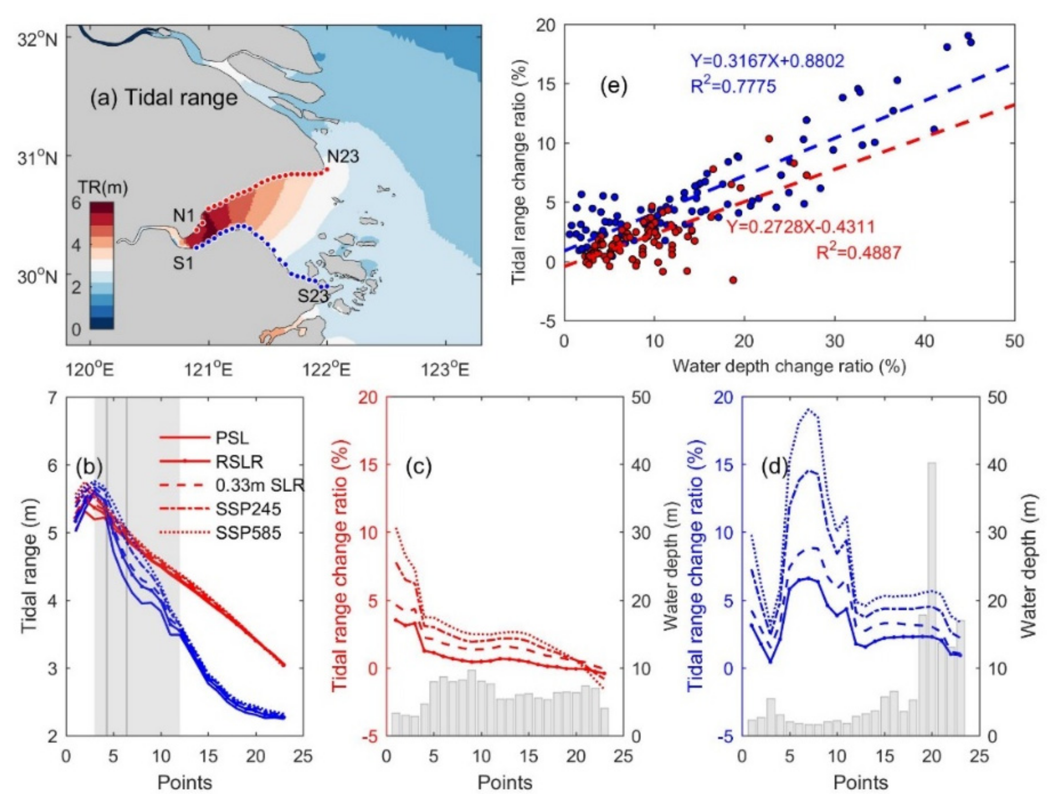
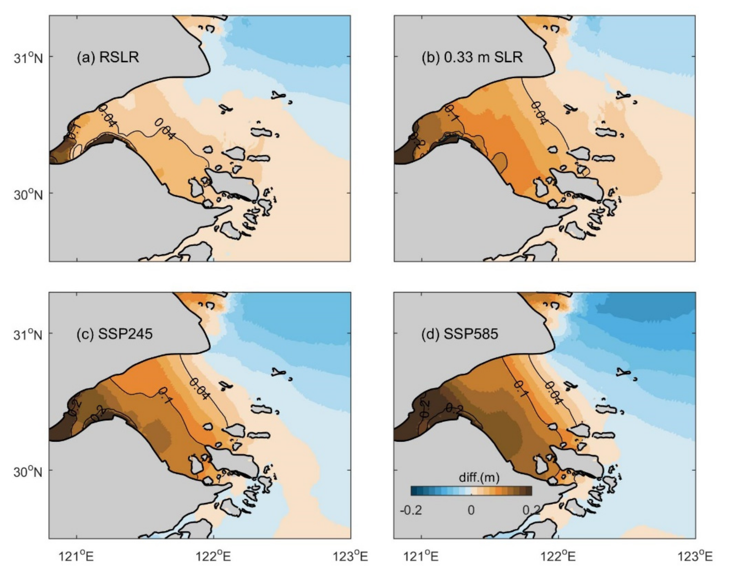
3.1. Responses of Tidal Range to SLR
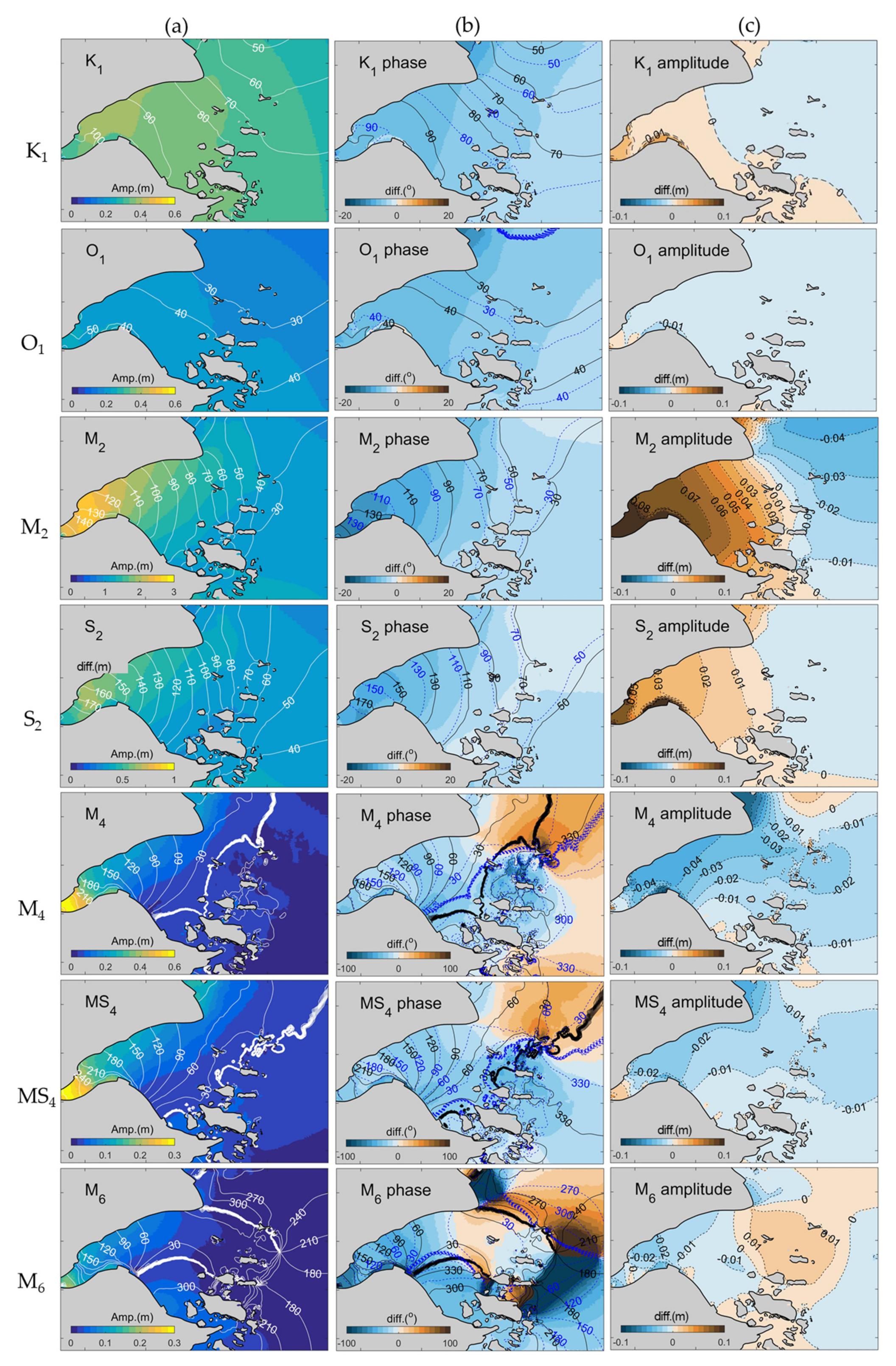
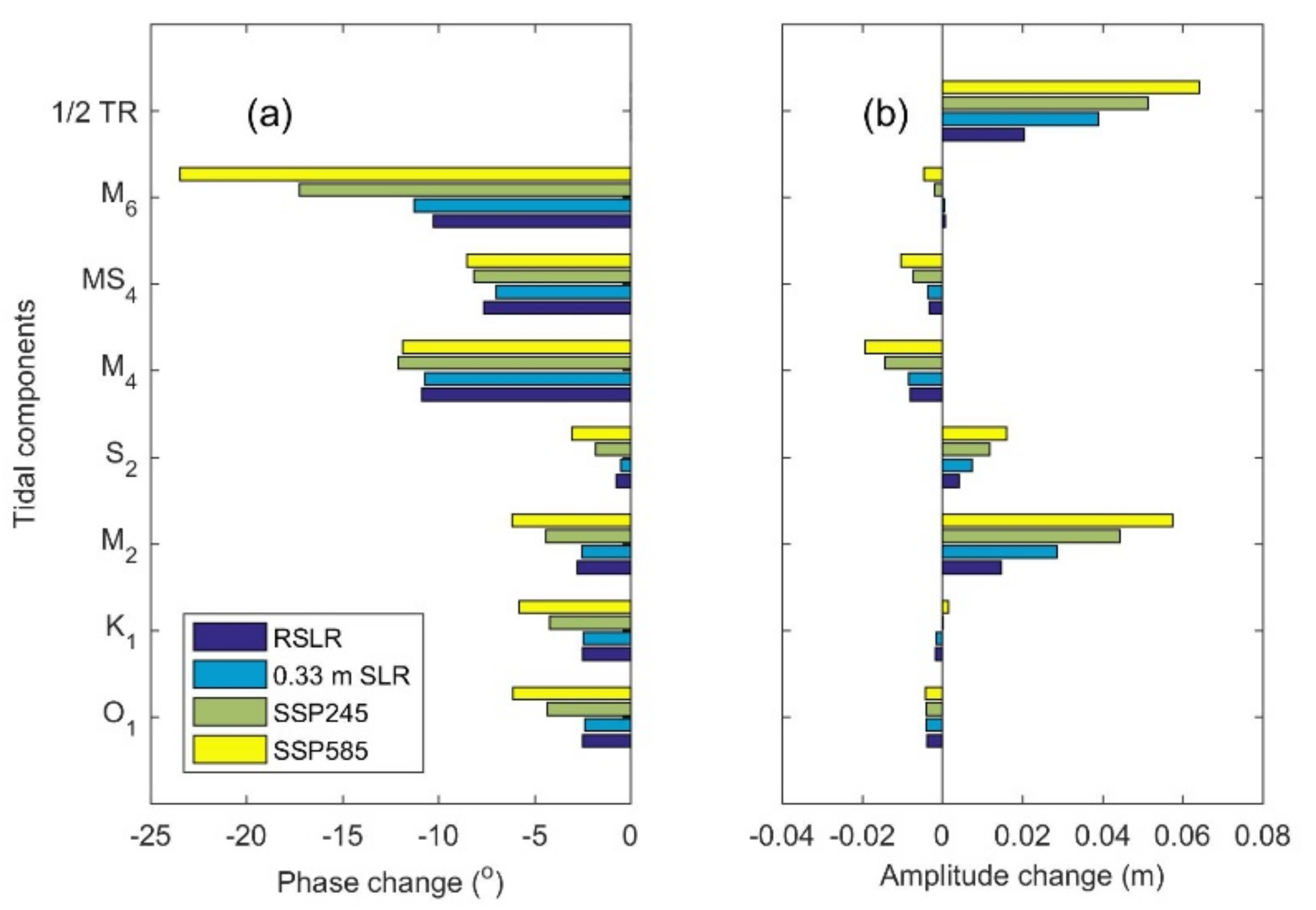
3.2. Tidal Components Behavior
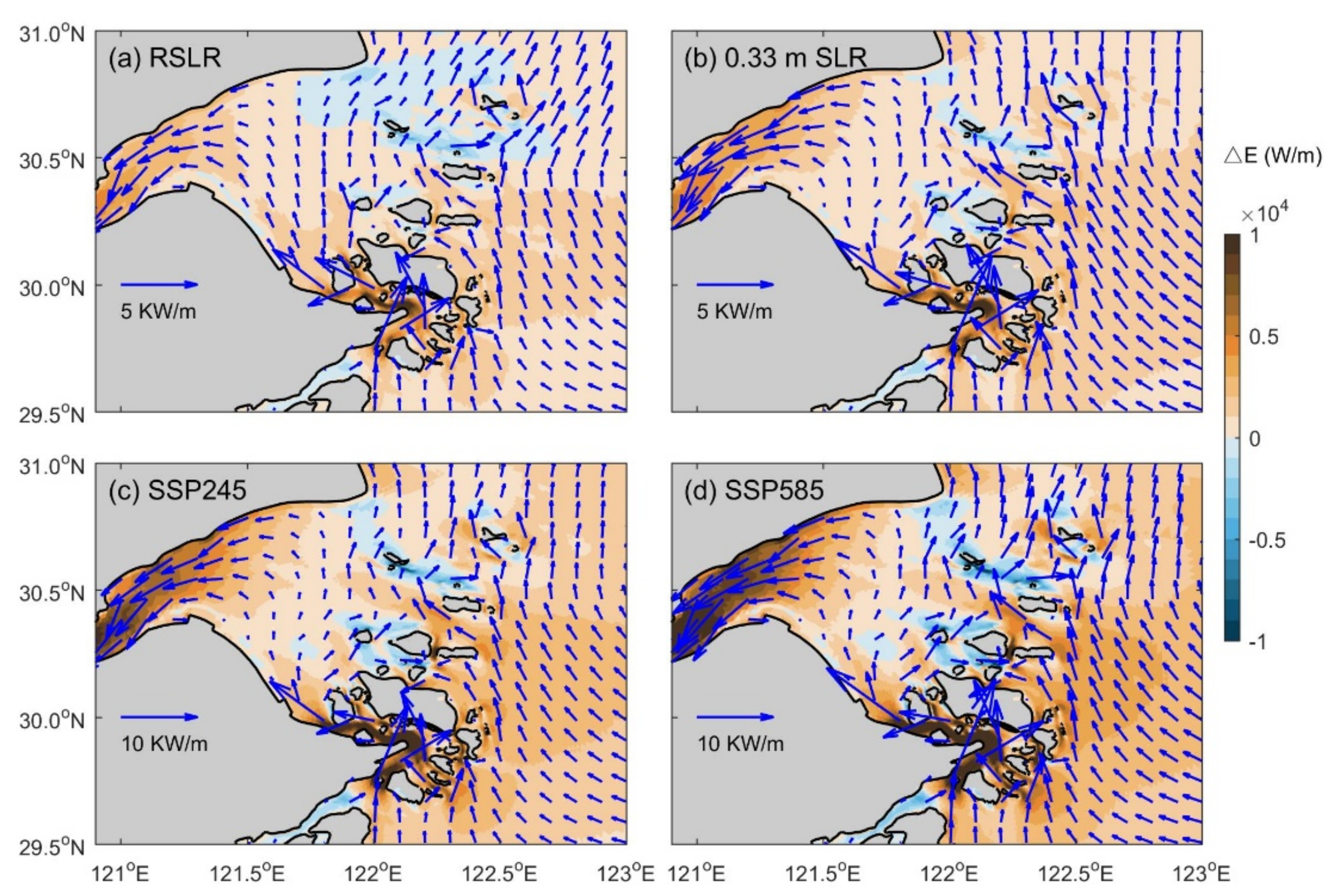
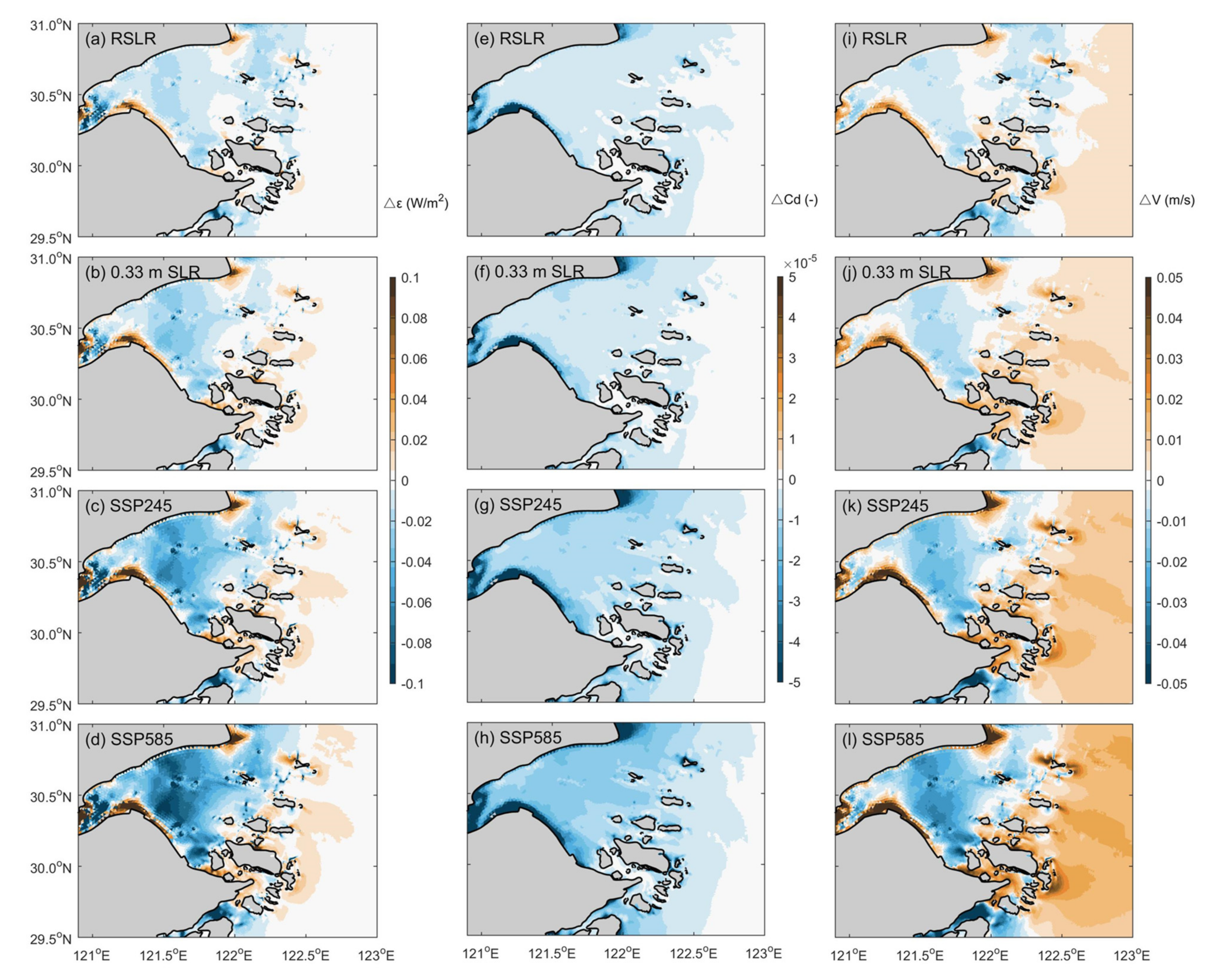
3.3. Tidal Energy Flux and Dissipation
3.3.1. Energy Budget in PSL Scenario
3.3.2. Responses to SLR
4. Discussion
4.1. Role of ZA on the Tidal Modification
4.2. Standing Environment and Tidal Flux Variation
4.3. Physical Mechanism for the Enhance of Progressive Waves around ZA
4.4. Comparison with Previous Studies
5. Conclusions
Author Contributions
Funding
Institutional Review Board Statement
Informed Consent Statement
Data Availability Statement
Acknowledgments
Conflicts of Interest
Appendix A

Appendix B
Appendix B.1. Tidal Energy Budget
Appendix B.2. Tidal Damping due to Bottom Dissipation
Appendix B.3. Tidal Phase Analysis (an Index to Quantify the Reflection Effect)
Appendix B.4. Momentum Balance
References
- Cazenave, A.; Dieng, H.; Meyssignac, B.; von Schuckmann, K.; Decharme, B.; Berthier, E. The rate of sea-level rise. Nat. Clim. Change 2014, 4, 358–361. [Google Scholar] [CrossRef]
- Fox-Kemper, B.; Hewitt, H.T.; Xiao, C.; Aðalgeirsdóttir, G.; Drijfhout, S.S.; Edwards, T.L.; Golledge, N.R.; Hemer, M.; Kopp, R.E.; Krinner, G.; et al. Ocean, Cryosphere and Sea Level Change. In Climate Change 2021: The Physical Science Basis; Cambridge University Press: Cambridge, UK, 2021. [Google Scholar]
- Silveira, F.; Lopes, C.L.; Pinheiro, J.P.; Pereira, H.; Dias, J.M. Coastal floods induced by mean sea level rise—Ecological and socioeconomic impacts on a mesotidal lagoon. J. Mar. Sci. Eng. 2021, 9, 1430. [Google Scholar] [CrossRef]
- Anwar, M.S.; Rahman, K.; Md, A.E.B.; Saha, R. Assessment of sea level and morphological changes along the eastern coast of Bangladesh. J. Mar. Sci. Eng. 2022, 10, 527. [Google Scholar] [CrossRef]
- Jabir, A.; Hasan, G.M.J.; Anam, M.M. Correlation between temperature, sea level rise and land loss: An assessment along the Sundarbans coast. J. King Saud Univ. Eng. Sci. 2021, in press. [Google Scholar] [CrossRef]
- Arns, A.; Wahl, T.; Dangendorf, S.; Jensen, J. The impact of sea level rise on storm surge water levels in the northern part of the German Bight. Coast. Eng. 2015, 96, 118–131. [Google Scholar] [CrossRef]
- Warner, N.N.; Tissot, P.E. Storm flooding sensitivity to sea level rise for Galveston Bay, Texas. Ocean Eng. 2012, 44, 23–32. [Google Scholar] [CrossRef]
- Rose, L.; Bhaskaran, P.K. Tidal variations associated with sea level changes in the Northern Bay of Bengal. Estuar. Coast. Shelf Sci. 2022, 272, 107881. [Google Scholar] [CrossRef]
- Bacopoulos, P.; Hagen, S.C. Dynamic considerations of sea-level rise with respect to water levels and flooding in Apalachicola Bay. J. Coast. Res. 2014, 68, 43–48. [Google Scholar] [CrossRef]
- De Dominicis, M.; Wolf, J.; Jevrejeva, S.; Zheng, P.; Hu, Z. Future interactions between sea level rise, tides, and storm surges in the world’s largest urban area. Geophys. Res. Lett. 2020, 47, e2020GL087002. [Google Scholar] [CrossRef] [Green Version]
- Khan, M.J.U.; Durand, F.; Testut, L.; Krien, Y.; Islam, A.K.M.S. Sea level rise inducing tidal modulation along the coasts of Bengal delta. Cont. Shelf Res. 2020, 211, 104289. [Google Scholar] [CrossRef]
- Liu, K.X.; Wang, H.; Fu, S.J.; Gao, Z.G.; Dong, J.X.; Feng, J.L.; Gao, T. Evaluation of sea level rise in Bohai Bay and associated responses. Adv. Clim. Change Res. 2017, 8, 48–56. [Google Scholar] [CrossRef]
- Pelling, H.E.; Uehara, K.; Green, J.A.M. The impact of rapid coastline changes and sea level rise on the tides in the Bohai Sea, China. J. Geophys. Res. Ocean. 2013, 118, 3462–3472. [Google Scholar] [CrossRef] [Green Version]
- Passeri, D.L.; Hagen, S.C.; Medeiros, S.C.; Bilskie, M.V. Impacts of historic morphology and sea level rise on tidal hydrodynamics in a microtidal estuary (Grand Bay, Mississippi). Cont. Shelf Res. 2015, 111, 150–158. [Google Scholar] [CrossRef] [Green Version]
- Kuang, C.; Liang, H.; Mao, X.; Karney, B.; Gu, J.; Huang, H.; Chen, W.; Song, H. Influence of potential future sea-level rise on tides in the China Sea. J. Coast. Res. 2017, 331, 105–117. [Google Scholar] [CrossRef]
- Khojasteh, D.; Hottinger, S.; Felder, S.; De Cesare, G.; Heimhuber, V.; Hanslow, D.J.; Glamore, W. Estuarine tidal response to sea level rise: The significance of entrance restriction. Estuar. Coast. Shelf Sci. 2020, 244, 106941. [Google Scholar] [CrossRef]
- Haigh, I.D.; Pickering, M.D.; Green, J.A.M.; Arbic, B.K.; Arns, A.; Dangendorf, S.; Hill, D.F.; Horsburgh, K.; Howard, T.; Idier, D.; et al. The tides they are a-changin’; A comprehensive review of past and future nonastronomical changes in tides, their driving mechanisms, and future implications. Rev. Geophys. 2019, 58, e2018RG000636. [Google Scholar] [CrossRef] [Green Version]
- Payandeh, A.R.; Justic, D.; Huang, H.; Mariotti, G.; Hagen, S.C. Tidal change in response to the relative sea level rise and marsh accretion in a tidally chocked estuary. Cont. Shelf Res. 2022, 234, 104642. [Google Scholar] [CrossRef]
- Hou, F.; Bao, X.W.; Li, B.X.; Liu, Q.Q. The assessment of extractable tidal energy and the effect of tidal energy turbine deployment on the hydrodynamics in Zhoushan. Acta Oceanol. Sin. 2015, 34, 86–91. [Google Scholar] [CrossRef]
- Li, Y.; Pan, D. The ebb and flow of tidal barrage development in Zhejiang Province, China. Renew. Sustain. Energy Rev. 2017, 80, 380–389. [Google Scholar] [CrossRef]
- Feng, J.; Li, W.; Wang, H.; Zhang, J.; Dong, J. Evaluation of sea level rise and associated responses in Hangzhou Bay from 1978 to 2017. Adv. Clim. Change Res. 2018, 9, 227–233. [Google Scholar] [CrossRef]
- Pan, C.; Zheng, J.; Wu, G.; Chen, G. Spatiotemporal variation of annual maximum high tide levels and reason analysis for their uplifting in Hangzhou Bay. J. Hohai Univ. Nat. Sci. 2021, 49, 394–400. (In Chinese) [Google Scholar]
- Liu, Y.; Xia, X.; Chen, S.; Jia, J.; Cai, T. Morphological evolution of Jinshan Trough in Hangzhou Bay (China) from 1960 to 2011. Estuar. Coast. Shelf Sci. 2017, 198, 367–377. [Google Scholar] [CrossRef]
- Wu, R.; Jiang, Z.; Li, C. Revisiting the tidal dynamics in the complex Zhoushan Archipelago waters: A numerical experiment. Ocean Model. 2018, 132, 139–156. [Google Scholar] [CrossRef]
- Xie, D. Modeling the morphodynamic response of a large tidal channel system to the large-scale embankment in the Hangzhou Bay, China. Anthr. Coasts 2018, 1, 89–100. [Google Scholar] [CrossRef]
- Rong, Z.; Li, M. Tidal effects on the bulge region of Changjiang River plume. Estuar. Coast. Shelf Sci. 2012, 97, 149–160. [Google Scholar] [CrossRef]
- Xie, D.; Pan, C.; Gao, S.; Wang, Z.B. Morphodynamics of the Qiantang Estuary, China; controls of river flood events and tidal bores. Mar. Geol. 2018, 406, 27–33. [Google Scholar] [CrossRef]
- Guo, Y.; Zhang, J.; Zhang, L.; Shen, Y. Computational investigation of typhoon-induced storm surge in Hangzhou Bay, China. Estuar. Coast. Shelf Sci. 2009, 85, 530–536. [Google Scholar] [CrossRef]
- Wang, S.; Ge, J.; Meadows, M.E.; Wang, Z. Reconstructing a late Neolithic extreme storm event on the southern Yangtze coast, East China, based on sedimentary records and numerical modeling. Mar. Geol. 2022, 443, 106687. [Google Scholar] [CrossRef]
- Matsumoto, K.; Takanezawa, T.; Ooe, M. Ocean tide models developed by assimilating TOPEX/POSEIDON altimeter data into hydrodynamical model: A global model and a regional model around Japan. J. Oceanogr. 2000, 56, 567–581. [Google Scholar] [CrossRef]
- Feng, X.; Feng, H.; Li, H.; Zhang, F.; Feng, W.; Zhang, W.; Yuan, J. Tidal responses to future sea level trends on the Yellow Sea shelf. J. Geophys. Res. Ocean. 2019, 124, 7285–7306. [Google Scholar] [CrossRef]
- Roy, K.; Peltier, W.R. Relative sea level in the Western Mediterranean basin: A regional test of the ICE-7G_NA (VM7) model and a constraint on Late Holocene Antarctic deglaciation. Quat. Sci. Rev. 2018, 183, 76–87. [Google Scholar] [CrossRef]
- Holleman, R.C.; Stacey, M.T. Coupling of Sea Level Rise, Tidal Amplification, and Inundation. J. Phys. Oceanogr. 2014, 44, 1439–1455. [Google Scholar] [CrossRef]
- Hench, J.L.; Luettich, R.A. Transient tidal circulation and momentum balances at a shallow inlet. J. Phys. Oceanogr. 2003, 33, 913–932. [Google Scholar] [CrossRef]
- Guo, W.; Wang, X.H.; Ding, P.; Ge, J.; Song, D. A system shift in tidal choking due to the construction of Yangshan Harbour, Shanghai, China. Estuar. Coast. Shelf Sci. 2017, 206, 49–60. [Google Scholar] [CrossRef]
- Gu, Y. Influence of Island Connecting Project and Sea Level Rise on Sediment Transport Mechanism in Zhoushan Sea Area; Zhejiang Ocean University: Zhoushan, China, 2020; 79p. [Google Scholar]
- Zhang, W.S.; Zhang, J.S.; Lin, R.D.; Zong, H.C. Tidal response of sea level rise in marginal seas near China. Adv. Water Sci. 2013, 24, 243–250. [Google Scholar]
- Chen, W.; Chen, K.; Kuang, C.; Zhu, D.Z.; He, L.; Mao, X.; Liang, H.; Song, H. Influence of sea level rise on saline water intrusion in the Yangtze River Estuary, China. Appl. Ocean Res. 2016, 54, 12–25. [Google Scholar] [CrossRef]
- Pan, C.; Zheng, J.; Cheng, G.; He, C.; Tang, Z. Spatial and temporal variations of tide characteristics in Hangzhou Bay and cause analysis. Ocean. Eng. 2019, 37, 1–11. [Google Scholar]
- Pan, C.; Zheng, J.; Zeng, J.; Chen, G. Analysis of annual maximum tidal range in Hangzhou Bay. J. Hydrodyn. 2021, 36, 201–209. [Google Scholar]
- Meng, W.; Hu, B.; He, M.; Liu, B.; Mo, X.; Li, H.; Wang, Z.; Zhang, Y. Temporal-spatial variations and driving factors analysis of coastal reclamation in China. Estuar. Coast. Shelf Sci. 2017, 191, 39–49. [Google Scholar] [CrossRef]
- Li, L.; Ye, T.; Wang, X.H.; He, Z.; Shao, M. Changes in the Hydrodynamics of Hangzhou Bay Due to Land Reclamation in the Past 60 Years. In Sediment Dynamics of Chinese Muddy Coasts and Estuaries. Physics, Biology and Their Interactions; Academic Press: Cambridge, MA, USA, 2019; pp. 77–93. [Google Scholar]
- Shan, S.; Hannah, C.G.; Wu, Y. Response of sea level to tide, atmospheric pressure, wind forcing and river discharge in the Kitimat Fjord System. Estuar. Coast. Shelf Sci. 2020, 246, 107025. [Google Scholar] [CrossRef]
- Kuang, C.; Chen, W.; Gu, J.; Su, T.; Song, H.; Ma, Y.; Dong, Z. River discharge contribution to sea-level rise in the Yangtze River Estuary, China. Cont. Shelf Res. 2017, 134, 63–75. [Google Scholar] [CrossRef]
- Xie, D.; Wang, Z.B.; Huang, J.; Zeng, J. River, tide and morphology interaction in a macro-tidal estuary with active morphological evolutions. Catena 2022, 212, 106131. [Google Scholar] [CrossRef]
- Willmott, C.J. On the validation of models. Phys. Geogr. 1981, 2, 184–194. [Google Scholar] [CrossRef]


| Energy Flux | Total Energy Dissipation | Bottom Friction Dissipation | ||||||
|---|---|---|---|---|---|---|---|---|
| S1 | S2 | S3 | S4 | S5 | ||||
| PSL | Total energy flux | 765.3 | 1056.5 | 1877.1 | 1275.1 | −944.2 | 4029.8 | 3805.8 |
| Kinetic part | 1.1 | −8.6 | 4.0 | 13.0 | −20.8 | |||
| Potential part | 764.2 | 1065.1 | 1873.0 | 1262.2 | −923.4 | |||
| RSLR | Total energy flux | 786.7 | 1071.1 | 1876.6 | 1247.0 | −998.7 | 3982.6 | 3757.0 |
| Kinetic part | 0.8 | −9.4 | 0.2 | 7.1 | −20.4 | |||
| Potential part | 785.9 | 1080.5 | 1876.4 | 1239.9 | −978.3 | |||
| 0.33 m SLR | Total energy flux | 787.2 | 1048.6 | 1879.7 | 1262.5 | −1012.3 | 3965.6 | 3737.4 |
| Kinetic part | 1.0 | −9.1 | 0.8 | 8.0 | −20.8 | |||
| Potential part | 786.2 | 1057.7 | 1878.9 | 1254.5 | −991.5 | |||
| SSP245 | Total energy flux | 800.0 | 1038.0 | 1873.8 | 1245.5 | −1064.6 | 3892.8 | 3662.4 |
| Kinetic part | 1.3 | −8.5 | 1.4 | 7.1 | −21.8 | |||
| Potential part | 798.7 | 1046.5 | 1872.4 | 1238.5 | −1042.8 | |||
| SSP585 | Total energy flux | 811.4 | 1027.3 | 1864.8 | 1225.0 | −1110.0 | 3818.5 | 3586.4 |
| Kinetic part | 1.6 | −8.1 | 2.1 | 6.2 | −22.5 | |||
| Potential part | 809.8 | 1035.3 | 1862.7 | 1218.9 | −1087.6 | |||
| Stations | φc (o) | Local Acceleration (In x Direction/In y Direction) | Advection (In x Direction/In y Direction) | Coriolis (In x Direction/In y Direction) | Barotropic (In x Direction/In y Direction) | Friction (In x Direction/In y Direction) |
|---|---|---|---|---|---|---|
| S1 | 1.9 | 8.9/5.5 | 6.4/9.8 | 2.9/4.6 | 16.1/11.5 | 1.4/0.9 |
| S2 | 15.2 | 8.4/1.0 | 10.9/3.0 | 0.5/4.4 | 16.9/3.7 | 1.2/0.1 |
| S3 | 17.9 | 11.6/7.5 | 30.3/3.8 | 4.0/6.2 | 26.4/8.5 | 3.5/2.2 |
| S4 | 11.3 | 5.0/6.3 | 12.9/4.2 | 3.5/2.6 | 12.8/7.2 | 0.6/0.8 |
| S5 | 87.6 | 13.7/5.8 | 2.0/4.7 | 2.9/7.1 | 19.8/7.8 | 10.1/4.2 |
| Stations | φc (o) | Local Acceleration (In x Direction/In y Direction) | Advection (In x Direction/In y Direction) | Coriolis (In x Direction/In y Direction) | Barotropic (In x Direction/In y Direction) | Friction (In x Direction/In y Direction) |
|---|---|---|---|---|---|---|
| S1 | 19.8 | 5.0/7.1 | 0.9/3.2 | 3.7/2.7 | 5.8/7.4 | 0.7/1.0 |
| S2 | 39.7 | 8.4/4.8 | 3.9/1.7 | 2.6/4.4 | 9.7/5.6 | 1.7/0.9 |
| S3 | 35.1 | 10.3/7.0 | 4.4/1.5 | 3.8/5.4 | 8.6/4.6 | 3.0/2.0 |
| S4 | 40.6 | 9.1/5.3 | 2.4/0.9 | 2.9/4.7 | 6.9/2.4 | 1.8/1.0 |
| S5 | 88.9 | 15.2/6.7 | 2.7/6.7 | 3.3/8.0 | 25.2/9.6 | 13.1/5.5 |
Publisher’s Note: MDPI stays neutral with regard to jurisdictional claims in published maps and institutional affiliations. |
© 2022 by the authors. Licensee MDPI, Basel, Switzerland. This article is an open access article distributed under the terms and conditions of the Creative Commons Attribution (CC BY) license (https://creativecommons.org/licenses/by/4.0/).
Share and Cite
Liang, H.; Chen, W.; Liu, W.; Cai, T.; Wang, X.; Xia, X. Effects of Sea Level Rise on Tidal Dynamics in Macrotidal Hangzhou Bay. J. Mar. Sci. Eng. 2022, 10, 964. https://doi.org/10.3390/jmse10070964
Liang H, Chen W, Liu W, Cai T, Wang X, Xia X. Effects of Sea Level Rise on Tidal Dynamics in Macrotidal Hangzhou Bay. Journal of Marine Science and Engineering. 2022; 10(7):964. https://doi.org/10.3390/jmse10070964
Chicago/Turabian StyleLiang, Huidi, Wei Chen, Wenlong Liu, Tinglu Cai, Xinkai Wang, and Xiaoming Xia. 2022. "Effects of Sea Level Rise on Tidal Dynamics in Macrotidal Hangzhou Bay" Journal of Marine Science and Engineering 10, no. 7: 964. https://doi.org/10.3390/jmse10070964
APA StyleLiang, H., Chen, W., Liu, W., Cai, T., Wang, X., & Xia, X. (2022). Effects of Sea Level Rise on Tidal Dynamics in Macrotidal Hangzhou Bay. Journal of Marine Science and Engineering, 10(7), 964. https://doi.org/10.3390/jmse10070964