Numerical Investigation of the Vibration of a Circular Cylinder in Oscillatory Flow in Oblique Directions

Abstract

The response of an elastically mounted circular cylinder vibrating in an oscillatory flow oblique to the flow direction is investigated. Simulations are conducted for vibration angles ranging from 0° to 90°, with 0° and 90° corresponding to the cases where the vibration is inline and perpendicular to the flow direction, respectively. One mass ratio of 2, one Reynolds number of 150, and two Keulegan–Carpenter (KC) numbers of 5 and 10 and a wide range of frequency ratios that cover the lock-in regime are considered. The frequency ratio is the ratio of the oscillatory flow frequency to the natural frequency. The maximum vibration amplitude is highest when the cylinder vibrates in the flow direction (vibration angle = 0°) and gradually decreases with the increase of the vibration direction. All the identified flow regimes are mapped on the frequency ratio versus vibration angle space. In addition to the flow regimes that exist for a stationary cylinder, two variants of Regime F (F1 and F2), a new flow regime R and an unstable regime D/F are found. The vortex street directions of Regime F1 and F2 are the opposite to and the same as the direction of the vibration, respectively, Regime R is a regime where a dominant vortex circles around the cylinder and Regime D/F is an unstable regime where the flow changes between Regime D and F frequently. The contribution of the higher harmonics in the vibration increases with the increase of the vibration direction angle. As a result of the strong contribution of higher harmonics at large vibration angles and small frequency ratios, local peak values of the vibration amplitude are found at frequency ratios of 0.4 and 0.25 for KC = 5 and 10, respectively.

1. Introduction

The excessive flow-induced vibrations (FIV) of flexible structures in fluid flow can lead to material fatigue and eventually failure [1]. The main mechanism that causes the FIV of cylindrical structures is the formation and separation of vortices from structures. Vortex shedding from a circular cylinder in a steady flow occurs when the Reynolds number (Re) is greater than 47 [2]. As the Reynold number increases, the wake flow changes from laminar to turbulent and becomes totally turbulent when the Reynolds number is greater than 300. However the flow around the boundary layer is still laminar and becomes totally turbulent when $\mathrm{Re}>4\times {10}^6$ [3]. The dynamic forces due to the vortex shedding flow around a cylinder can make the cylinder undergo periodic oscillations [4]. The synchronization of the vortex shedding frequency and the vibration frequency of an object can result in large amplitudes of vibration, and this is referred to as “lock-in” [5]. The dynamic response of an elastically supported cylinder in fluid flow is influenced by its mass, stiffness and damping coefficient [6]. The maximum vibration amplitudes decrease with the increase in mass ratio [7,8] and decrease with the increase in damping ratio [9].

Ocean waves can be modeled by oscillatory flows in engineering applications. Research on the interaction between sinusoidally oscillatory flows and structures has viable applications in offshore engineering. The Keulegan–Carpenter ($KC$) number is a key parameter that controls the mechanisms of the interaction between oscillatory flow and structures. The KC number for a sinusoidally oscillatory flow past a circular cylinder is defined as $KC=U_{m}T/D$, where D is the diameter of the cylinder and U_m and T are the velocity amplitude and the period of the oscillatory flow, respectively. Vortex flow patterns in oscillatory flow are reliant on both Reynolds number and KC number [10]. An increase in KC with a constant Reynold number can change the flow from laminar to turbulent [11]. In oscillatory flow, the minimum KC required for the generation of vortices is 1.1, and the vortices are generated every half-period of the flow [11].

The fluid motion amplitude (a) is related to the KC number by $a=KC·D/2\pi$, and the ratio of the Reynolds number to the KC number is defined as the Stokes number, $\beta =Re/KC$. Tatsuno and Bearman [12] experimentally studied flow around a cylinder in oscillatory flow. They identified and mapped out eight different flow regimes based on the flow patterns near the cylinder. Vortex shedding patterns can also be classified based on the number of vortices that are shed from the cylinder in one period of flow. The vortex shedding pattern is referred to as “2S” if a single vortex is shed in every half-period and “2P” if a pair of vortices are shed per half-period [13]. The flow for a cylinder in oscillation may transition to three-dimensional at large KC numbers. The three-dimensionality of the flow affects the forces but dows not qualitatively affect the two-dimensional flow features [14]. Zhao and Cheng [15] conducted a detailed two-dimensional numerical study of flow past circular cylinders and reported all the flow features observed in the experiments. The butterfly-shaped vibration trajectory in the study of the vibration of a flexible, long circular cylinder in oscillatory flow by Fu et al. [16,17] also reported the two-dimensional study of the vibration of an elastically mounted rigid cylinder by Zhao [18]. Simulations with higher Reynolds numbers often consist of the changing of 2S and 2P modes, which is related to the shifting of the upper and lower branches of excitation [19].

Sumer and Fredsøe [20] found high vibration frequencies when a cylinder vibrated transervely in oscillatory flow. Vibration of a cylinder in the transverse direction in an oscillatory flow with KC = 10 has a single frequency when the reduced velocity is under 8 and multiple frequencies when reduced velocity is above 8 [21]. The reduced velocity is defined as $U_r=U_m/\left(f_{n}D\right),$ where $f_n$ is the natural freqency measured in a vacuum. Fu et al. [16] demonstrated that in oscillatory flow, a cylinders vibration amplitude increases as the reduced velocity increases up to a certain point and then decreases, and the ‘lock-in’ occurs for a range of reduced velocities. Taheri et al. [22] confined the vibration direction in the inline direction only and found the vortex shedding mode is dependent on the relative velocity between the cylinder and the flow. Taheri et al. [23] further investigated energy harvesting through the vibration of a cylinder in oscillatory flow and found the maximum power can be obtained when the natural frequency measured in water and the flow frequency synchronize.

The vibration of an elastically mounted rigid cylinder in both inline and crossflow directions in oscillatory flow happen to share similar characteristics with the vibration of a flexible cylinder. Neshamar et al. [24] and Deng et al. [25] reported that the vibration of a flexible cylinder and the vibration of an elastically mounted rigid cylinder have similar trajectories. While most of the numerical studies of vibration of a cylinder in oscillatory flow are conducted through two-dimensional numerical simulations, some alternate methods, such as the wake oscillator models, were also developed [26,27].

In offshore engineering, cylindrical structures may be supported in a way that they vibrate obliquely to the flow direction. Little to no research has been conducted to understand the response of a translationally vibrating cylinder in an oblique direction of an oscillatory flow. Bourguet [28] investigated the oblique vibration of a circular cylinder in steady flow. It was found that the vibration amplitude followed the typical lock-in pattern, hence the vibration amplitude increases to a peak and then decreases as the reduced velocity increases. Their findings also showed that, as the vibration angle increases from 0° to 90°, the lock-in range of reduced velocity widens. The vibration angles of 0° and 90° correspondto the cases where the vibration direction and the flow direction are parrallel and perpendicular to each other, respectively. Hans et al. [29] found that increasing the angle of vibration caused a reduction in the vibration amplitude of a cylinder in steady flow.

Based on the current literature, a lot of focus has been devoted to one-degree-of-freedom FIV in the crossflow direction, streamwise direction, or two-degrees-of-freedom vibration in both crossflow and inline directions in oscillatory flows. Little attention has been paid to one-degree-of-freedom FIV of a cylinder in an arbitrary direction in oscillatory flow. This paper invistigates the translational vibration of a cylinder in an oblique direction relative to an oscillatory flow, as indicated in Figure 1, through two-dimensional numerical simulations. The angle between the oscillatory flow and the vibration of the cylinder is defined as β. The effects of the direction angle β on the vibration amplitude and the flow patterns are examined by numercial simulations with a mass ratio of 2, a Reynolds number of 150, two KC numbers of 5 and 10 and β = 0° to 90°, with increments of 15° and a wide range of frequency ratios.

Although the flow at KC = 10 has become three-dimensional at Re = 150 [30], the weak three-dimensionality at such a small Reynolds number does not have effects on the fluid forces [31,32]. Taheri et al. [22], who used the same numerical model as used in this study, compared 2D and 3D numerical results of the vibration of a cylinder in the streamwise direction at Re = 150, and reported negligible difference between the 2D and 3D results in vibration displacement and the flow pattern on a cross-sectional plane. A two dimensional numerical model is used in this study, considering it is affordable to conduct a comprehensive study using a wide range of vibration directions and freqeuncy ratios.

2. Numerical Method

The cylinder is elastically mounted and vibrates in a sinusoidal oscillatory flow as shown in Figure 1. A cartesian coordinate system Oxy is defined with its origin located at the center of the static balance position of the circular cylinder, and the x-direction following the flow direction. The angle between the flow direction and the vibration direction of the cylinder is β. Another coordinate system, OXY, is defined with its x-diretion following the vibration direction of the cylinder. The velocity, the time and the pressure are nondimensionalized as $\left(u,v\right)=\left(\tilde{u},\tilde{v}\right)/U_m$, $t=\tilde{t}{U}_m/D$ and pressure $p=\tilde{p}/\left(\rho U_m^2\right)$, where u and v are the fluid velocity components in the x- and y-directions, respectively, $U_m$ is the amplitude of the oscillatory flow velocity, D is the cylinder diameter and p is the pressure. A tilde, ‘~’ on top of a variable represents a dimensional value. The cylinder elastically supported by a spring and a damper is only allowed to vibrate in the x-direction. The nondimensioinal incoming flow velocity is a sinsoidal function of time:

$$u=\sin \left(\sigma t\right)$$

(1)

where the nondimensional angular frequency of the flow is $\sigma =2\pi /KC$ and $KC=U_{m}T/D$ is the Keulegan–Carpenter (KC) number.

The incompressible two dimensional Navier–Stokes (NS) equations are used to simulate the fluid flow. To account for the continuous movement of the cylinder surface, the Arbitrary Lagrangian Eulerian (ALE) scheme is used to ensure the good quality of the computational mesh. The ALE allows the computational mesh inside the computational domain to move arbitrarily. Zhao et al. [33] proved the accuracy of simulating vibration of a cylinder in oscillatory flow through ALE. The NS equations are modified to account for the motion of the mesh in the ALE scheme, as such the nondimensional NS equations are [34]:

$$\frac{\partial u}{\partial x}+\frac{\partial v}{\partial y}=0$$

(2)

$$\frac{\partial u}{\partial t}+\left(u-\widehat{u}\right)\frac{\partial u}{\partial x}+\left(v-\widehat{v}\right)\frac{\partial u}{\partial y}=-\frac{\partial p}{\partial x}+\frac{1}{Re}(\frac{{\partial }^{2}u}{\partial x^2}+\frac{{\partial }^{2}u}{\partial y^2})$$

(3)

$$\frac{\partial v}{\partial t}+\left(u-\widehat{u}\right)\frac{\partial v}{\partial x}+\left(v-\widehat{v}\right)\frac{\partial v}{\partial y}=-\frac{\partial p}{\partial y}+\frac{1}{Re}(\frac{{\partial }^{2}v}{\partial x^2}+\frac{{\partial }^{2}v}{\partial y^2})$$

(4)

where the Reynolds number is defined as Re = U_mD/ν and ν is the kinematic viscosity of the fluid. In Equation (2), $\widehat{u}$ and $\widehat{v}$ are the nondimensional velocities of the moving mesh nodes in the x- and y-directions, respectively. The nondimensional displacement of the cylinder $X_c$ is calculated by solving the nondimensional motion equation:

$$\frac{d^2{X}_c}{d{t}^2}+\frac{4\pi \zeta }{U_r}\frac{d{X}_c}{dt}+\frac{4{\pi }^2}{U_r{}^2}{X}_c=\frac{2C_{FX}}{\pi m^{*}}$$

(5)

where C_FX is the nondimensional force in the X-direction, defined as $C_{FX}=F_X/\left(\rho D{U}_m^2/2\right)$, F_X is the fluid force in the X-direction, $m^{*}$ is the mass ratio (mass of the cylinder over the mass of the displaced fluid). A square shaped computational domain with a nondimensional boundary length of 110 is used and Figure 2 is the computational mesh near the cylinder. Anagnostopoulos and Minear [35] reported that the blockage effect on the force of a stationary cylinder in oscillatory flow is negligibly small if the blockage is lower than 20%. The blockage of 0.91% used in this study should be sufficiently small for blockage effect–free solutions.

The Petrov–Galerkin finite element method by Zhao et al. [36] is used to solve the NS equations. In the ALE scheme, the computational mesh needs to be moved based on the updated position of the cylinder. The displacements of the mesh nodes in the x- and y-directions are solved by the following equations [33]:

$$\nabla ·\left(\xi \nabla S_x\right)=0$$

(6)

$$\nabla ·\left(\xi \nabla S_y\right)=0$$

(7)

where $\epsilon$ is the parameter that control the mesh deformation. To make sure the small elements near the cylinder have small deformation, the parameter is chosen as $\xi =1/A_e$ in a finite element, where $A_{e }$ is the area of the element [33].

The surface of the cylinder is smooth and therefore a no-slip boundary condition is used that allows the fluid velocity on the surface of the cylinder to match the cylinders vibration velocity. A symmetric boundary condition is used on the top and bottom boundaries. On the left and right boundaries, the sinusoidal nondimensional flow velocity is given as $u\left(t\right)=\sin \left(\sigma t\right)$. The nondimensional pressure on the left and right boundaries is $p=-x\sigma \cos \left(\sigma t\right)$. The computational domain is divided into 37040 four-node quadrilateral finite elements, and the smallest size around the cylinders surface is 0.0008 (nondimensional radial size). The nondimensional computational time step is $\Delta t=0.0025$. The computational domain, mesh size and computational time step used in this paper are the same as those used by Taheri et al. [22], who used the same numerical model to simulate inline vibration of an elastically mounted circular cylinder in an oscillatory flow under same parameters as the current study. They obtained excellent agreement between the numerical results of the current model and the results calculated by the open-source Spectral/hp element code, Nektar++, by Cantwell et al. [37]. Because the mesh density used in this study is the same as the one used in Taheri et al. [22], numerical validation and mesh dependency studies were not repeated here.

3. Numerical Results

Flow Regimes

If the cylinder is stationary, the flows for a constant Re = 150 and various KC numbers can be classified into Regimes A/A*, D, F [12,15]. No vortices are generated or shed from the cylinder in Regime A*. In Regime A, two vortices form and are separated from the cylinder because of the flow reversal in each half cycle. Regime D has a pair of vortices that shed from one side of the cylinder in one cycle, forming an asymmetric flow pattern. In Regime F, two pairs of vortices are shed from the cylinder in one period of flow. If the cylinder can vibrate in the streamwise direction only at a constant KC = 10, the relative velocity of the fluid to the oscillatory cylinder changes with the change of frequency ratio. As a result, the above-mentioned flow regimes exist at a constant KC = 10 and various frequency ratios because flows at different frequency ratios have different effective KC numbers [22]. The frequency ratio is defined as the ratio of the oscillatory flow frequency to the natural frequency of the cylinder measured in a vacuum. When the cylinder oscillates diagonally in an oscillatory flow, we find three additional flow regimes: F1, F2 and R.

This section is arranged as follows. First, all the flow regimes for KC = 5 and 10 are mapped on the $f^{*}-\beta$ plane in Figure 3a,b, respectively. Then, detailed flow visualization of every flow regime mapped on Figure 3 is discussed. Simulations were conducted for β values ranging from 0° to 90° with an interval of 15° and the values of $f^{*}$ ranging from 0 to 4 with an interval of 0.25. As a result, the resolution of the boundaries between regimes is 15° in β and 0.25 in $f^{*}$. Because the flow near most of the boundaries between the regimes on the map is unstable and aperiodic, we did not further refine the resolution of the boundaries.

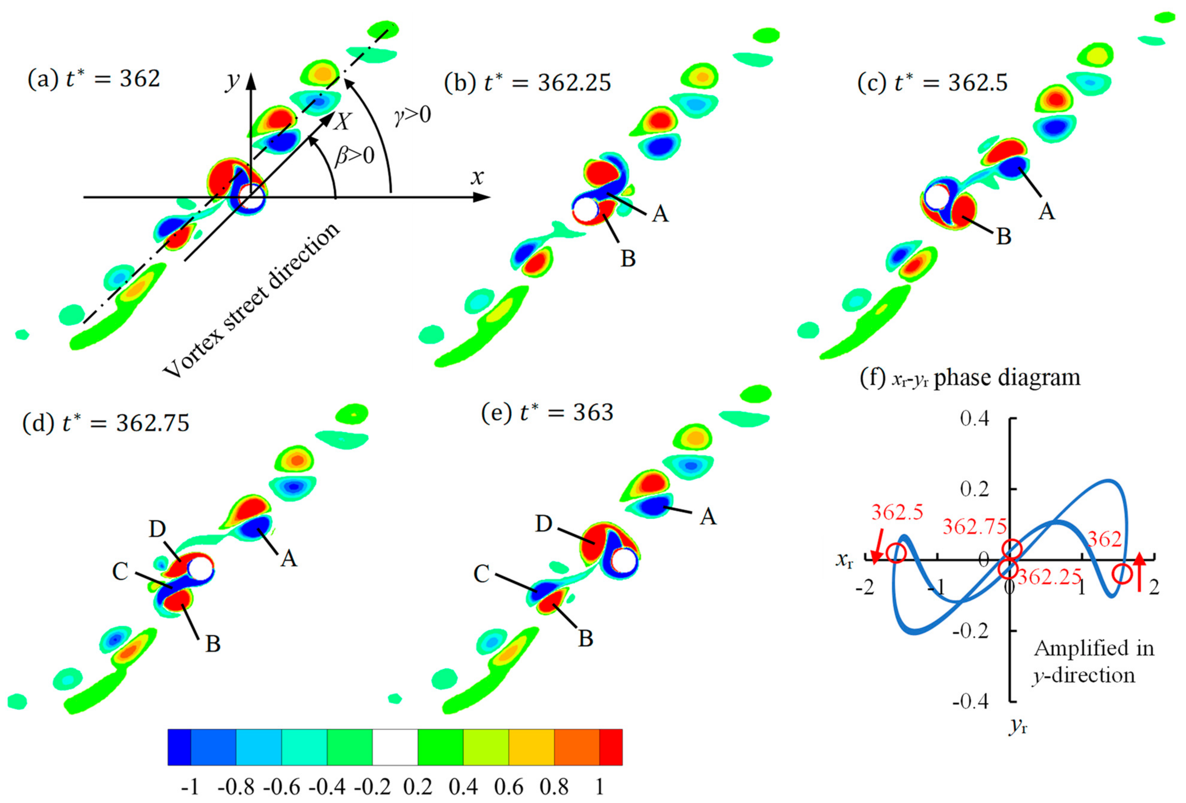
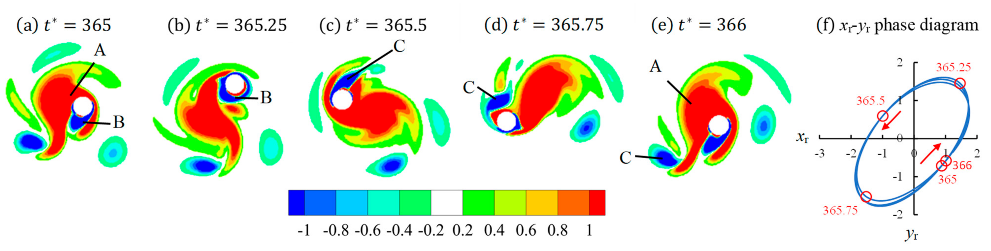
In Figure 3, KC = 10 and β = 45° have all the flow regimes except A/A*. This combination of KC and β are used as an example to explain all the flow regimes. Figure 4a–e uses contours of vorticity to show the flow patterns of Regime F1 for KC = 10, $f^{*}=0.2$ within one flow period. A vortex street alignment angle, γ, is defined as the angle between the vortex street direction and the positive x direction, as indicated in Figure 4a. The vortex street angle γ follows the anticlockwise direction. In regime F1, the vortex street direction angle is negative, i.e., opposite to the vibration direction angle. The flow regime F was found when the cylinder is stationary or vibrates in the streamwise direction (β = 0°). The regime F flow pattern at β = 0° is the same as the one shown in Figure 4, but the vortex street angle could be either positive or negative because of the symmetry of the configuration. In regime F1, two pairs of vortices (labeled as A to D in Figure 4) are shed from the cylinder in one period of flow and they are on two sides of the cylinders, respectively, forming a two-branch vortex street. After vortices B and D are shed from the cylinder before the flow reverses at t = 365.5 and 366, respectively, they are moved to another side of the cylinder by the reversed flow, while vortices A and C remain on the side of the cylinder where they are shed.

Figure 4f shows the relative displacement of the cylinder to the fluid. The nondimensional relative displacements in the x- and y-directions are defined as $x_r=X_c\cos \left(\beta \right)-x_f$ and $y_r=X_c\sin \left(\beta \right)-y_f$, where $x_f$ and $y_f$ are the nondimensional displacement of fluid particles calculated by $x_f=-\cos \left(\sigma t\right)/\sigma$ and $y_f=0$, respectively. The vortex flow pattern in Figure 4 is the same as Regime F in the stationary cylinder because the relative displacement $y_r$ is negligibly smaller than $x_r$, i.e., the cylinder vibrates nearly in the x-direction only relative to the fluid.

At KC = 10, Regime F1 occurs at very small frequency ratios for $\beta \ne 0°$ or $90°$, as shown in Figure 3. It does not occur at KC = 5. Increasing $f^{*}$ further for KC = 10 makes the flow change from F1 to F2 regime as shown in Figure 3b. The F2 regime is a variant of Regime F where the vortex street angle and the vibration direction angle are in the same direction as shown in Figure 5. Regimes F1 and F2 have the same flow patterns but different directions of vortex street alignment angle γ. In Regime F2, the first vortex A, which is shed in one oscillatory flow period, is a negative vortex from the top side of the cylinder, instead of a positive vortex from the top side, like in Regime F1. This difference in the vortex shedding sequence between Regimes F1 and F2 results in the difference in the direction of the vortex street angle. We conducted tests to find out if the flow is bistable or hysteresis, or dependent on the initial condition. In the test, we used the stabilized solution of Regime F1 at $f^{*}=0.2$ as the initial condition, changed the natural frequency of the cylinder to make $f^{*}=0.25$ and continued simulating the flow and found the flow developed to F2. We did the reverse test by using the stabilized flow pattern of F2 as the initial condition to simulate the case of F1, and the flow developed to F1. The above tests demonstrate Regime F1 and F2 are stable and they do not switch from one to another. We did the same test for other vibration direction angles and did not find F1–F2 bistable. Compared with Regime F1, the oscillation amplitude of $y_r$ is increased from 0.09 to 0.22 but is still much smaller than the amplitude of $x_r$. In addition, the phase between $x_r$ and $y_r$ of Regime F2 is different from Regime F1. For example, the directions of changing $y_r$ at maximum and minimum $x_r$ positions in Figure 4f are opposite to those in Figure 5f.

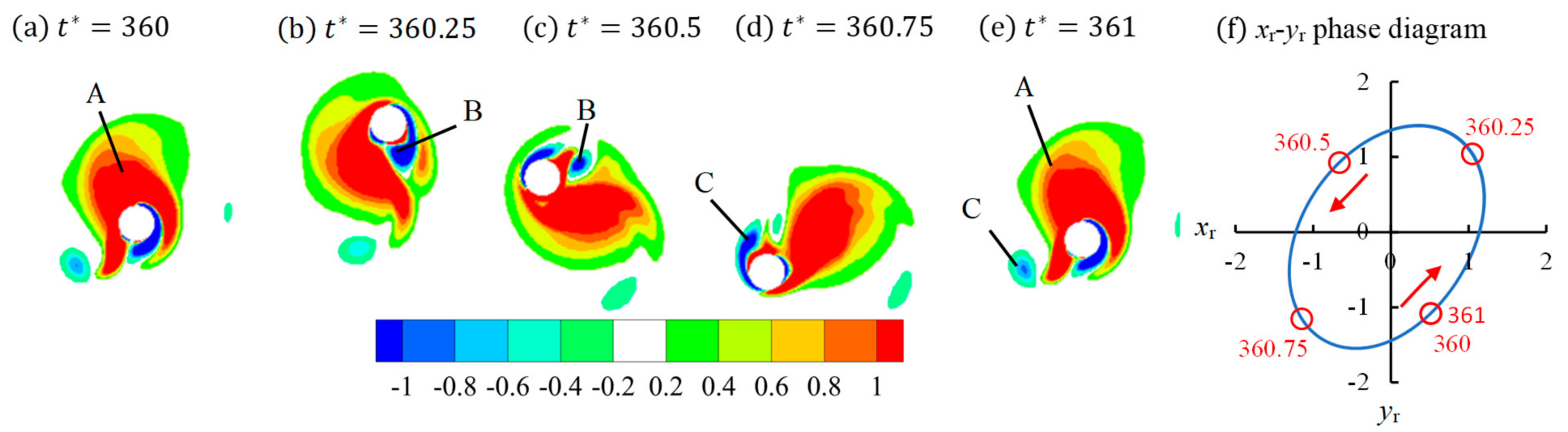
Figure 6 shows an example of Regime D, where a pair of vortices are shed from only one side of the cylinder in one period of flow and the flow pattern in this regime is also called a transverse vortex street [38]. Vortices A and B are shed from the cylinder within one flow period in Figure 6. All the vortices that are shed from the cylinder are located on the bottom side of the cylinder, forming a vortex street that is perpendicular to the flow direction. The vortices in Figure 6 are aligned in one vortex street and they dissipate much slower than the Regime D of a stationary cylinder [15].

By comparing Figure 4, Figure 5 and Figure 6, one can see that if Regime D, Regime F1 or F2 forms is determined by the behavior of the second shed vortex B within one period of flow. In regime F1 (see Figure 4c), the negative vortex B is fully cut off from the top side of the cylinder by the newly generated vortex C before the flow reverses. In the next half cycle, it moves towards the left on top of vortex C. The behavior of vortex B in regime F2 is the same only as vortex B in regime F1, but instead it is a negative vortex. In Regime D, the second vortex B in Figure 6 was generated but not shed from the cylinder. After vortex B in Figure 6c is generated from the top side of the cylinder, it moves along the cylinder surface from the top to the bottom side, instead of remaining on the top side, and it becomes the vortex that is shed from the second flow period.

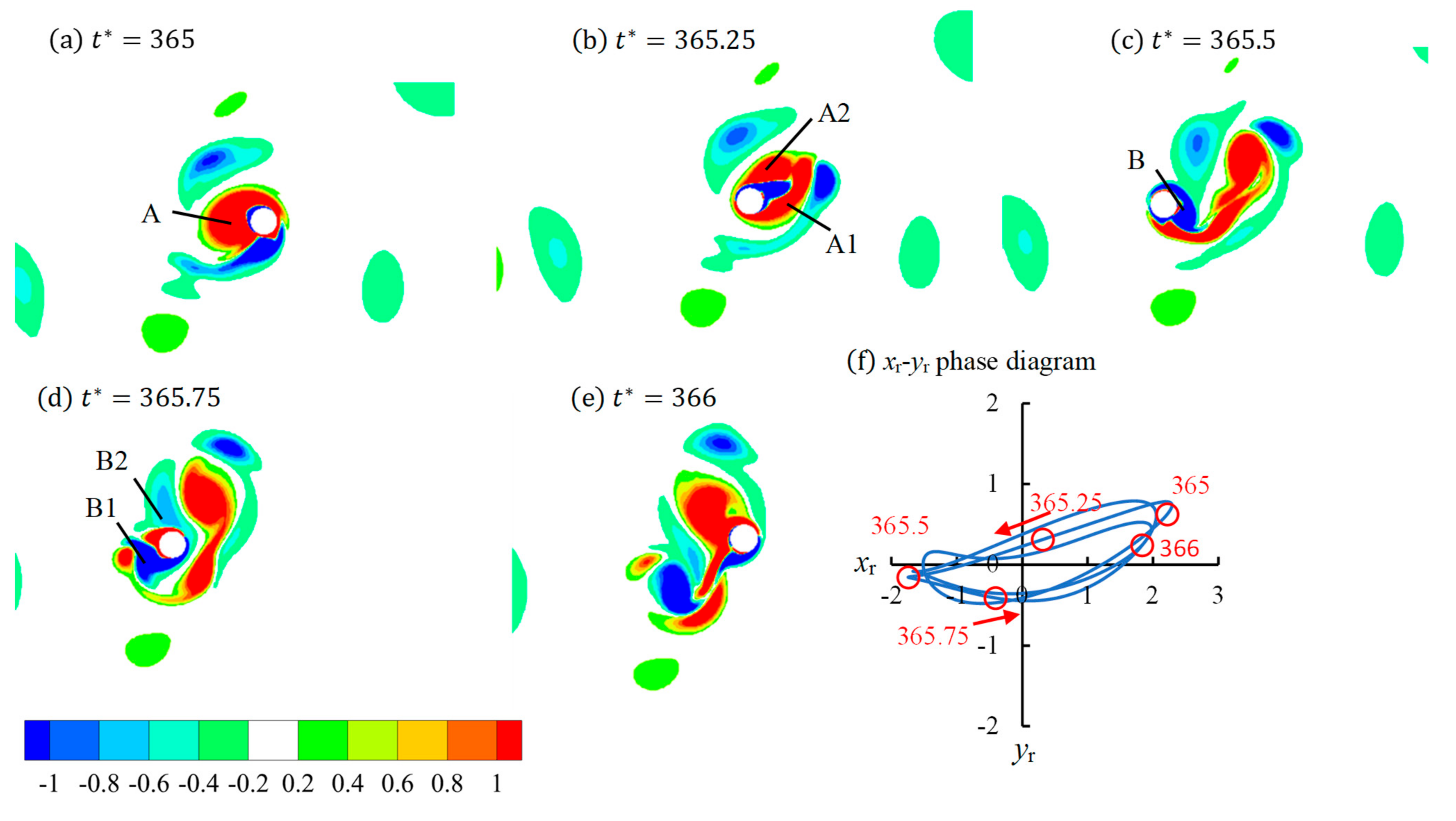
In Regimes F1, F2 and D, the second vortex in each half-period (i.e., vortex B) remains integral and moves along the cylinder surface, regardless of how it moves after the flow reverses. However, for some values of $f^{*}$, vortices clash with the cylinder every time after the flow reverses, resulting in an irregular vortex regime, which sometimes resembles Regime F and sometimes Regime D. This regime is defined as Regime D/F and some examples of this regime are shown in Figure 7 and Figure 8. In Figure 7, vortex A clashes with the cylinder after $t^{*}=365$ and is cut into two halves A1 and A2 by the cylinder at $t^{*}=365.25$ and vortex B is cut into a stronger B1 and a weaker B2 at $\left(\mathrm{a}\right) t^{*}=365.75$. If vortex A and B had not clashed with the cylinder moving into A1 and B1 positions, respectively, both A and B would have been shed from the bottom side of cylinder and formed a D regime. If vortex A and B had not clashed with the cylinder and moved to A2 and B2 positions, respectively, both A and B would have been shed from the top side of cylinder and formed an F regime. 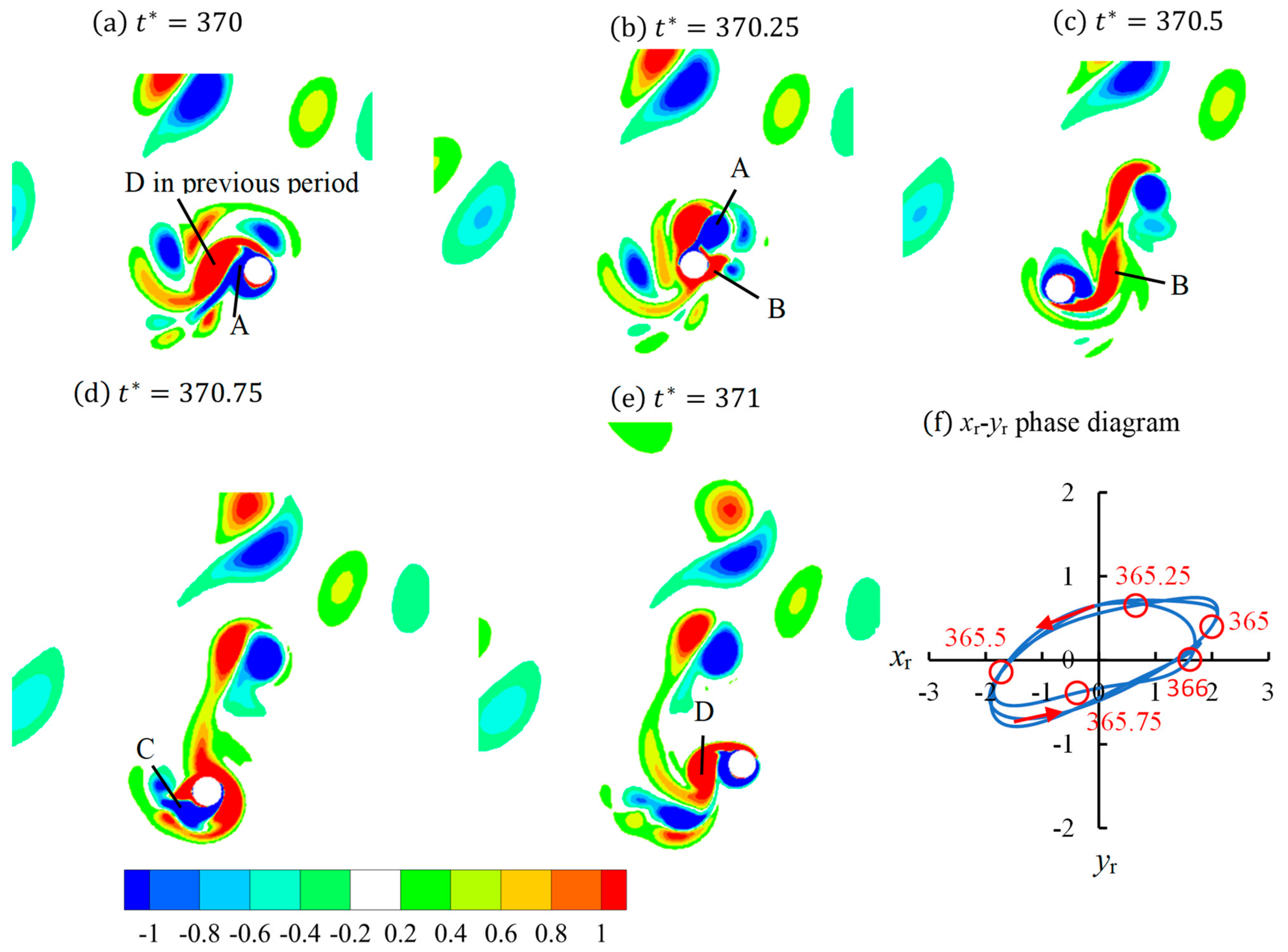Another example of Regime D/F is in Figure 8 where the vorticity contours for $f^{*}$=0.6 are shown. The vortex shedding pattern in Figure 8 resemble Regime F2, but in a very irregular shape. Vortices A and B are shed from the cylinder in the first half-period and vortices C and D are shed from the cylinder in the second half-period. The number of vortices that are shed from the cylinder in half-period is the same as the one in Figure 5 for Regime F2, but the vortices are not regularly arranged.

Regime D/F only occurs at KC = 10 and it occupies a greater area than Regimes D or F in the regime map in Figure 3. The flow is found to transition between Regimes D and F frequently in Regime D/F and the transition can be explained by the phase change of vortex shedding from period to period. Taking Figure 8 as an example, vortex D at t^* = 371 in Figure 8e is weaker than vortex D in the previous period (Figure 8a). In the transition Regime D/F, the last vortex that is shed from the cylinder at the end of period is found to either grow or shrink after each period. The growing and shrinking of a vortex at end of period could causes the flow transitioning from Regime D to F and F to D, respectively.

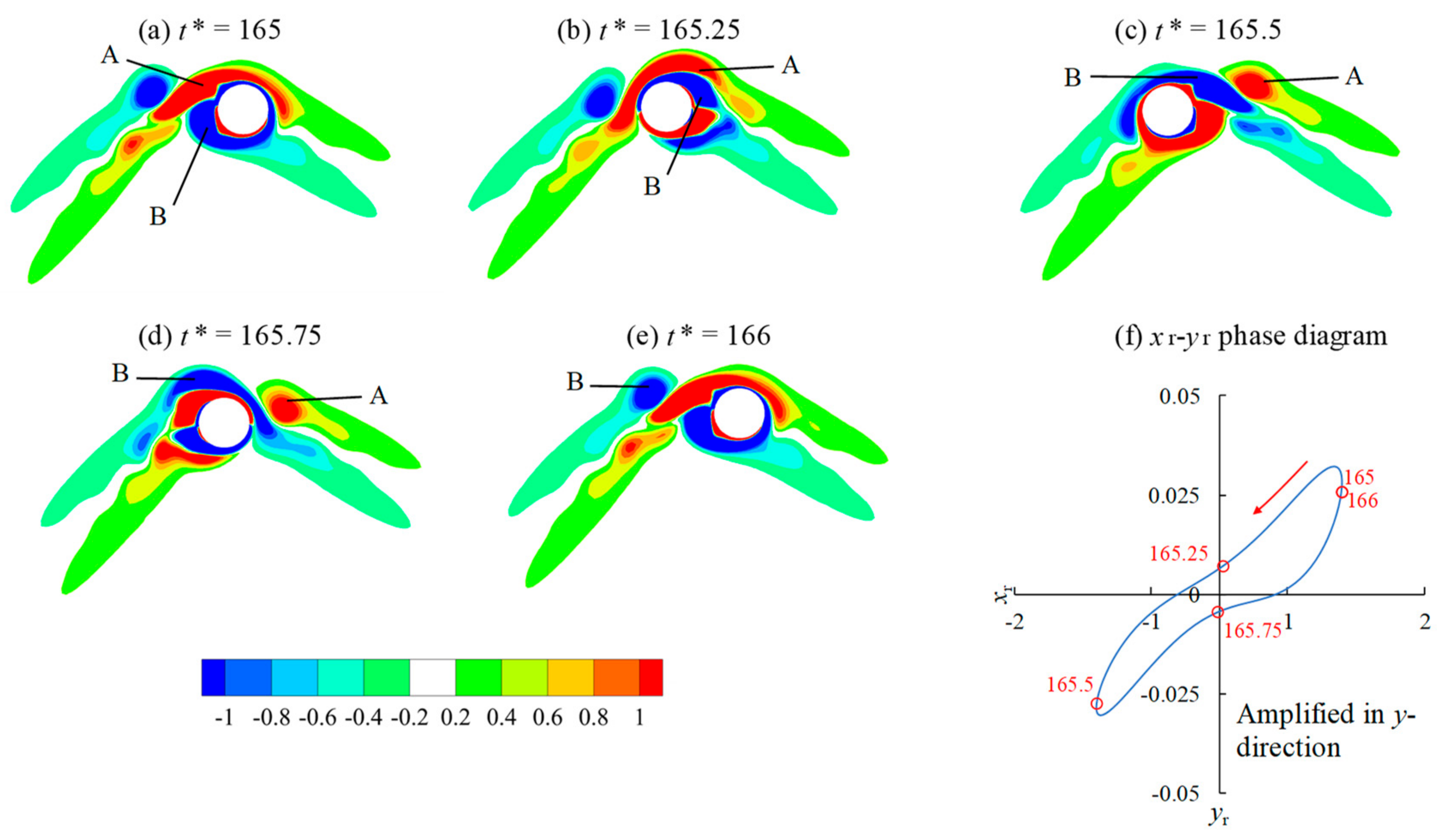
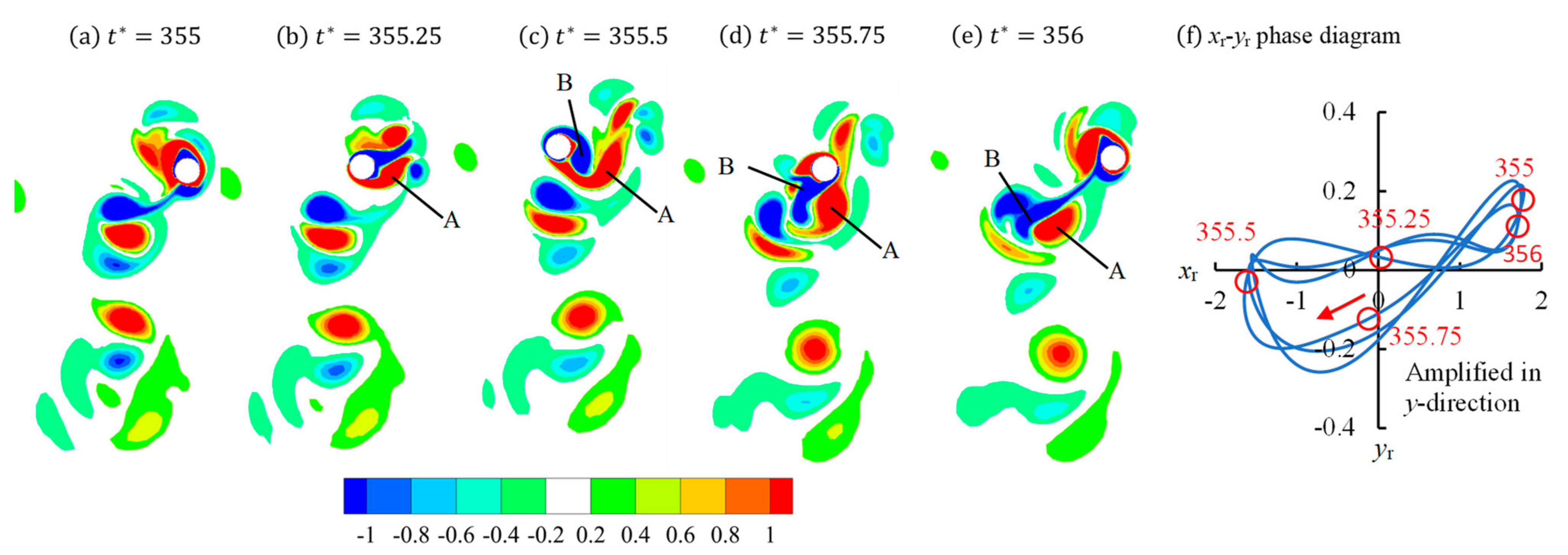
Regime R occupies the largest area in the regime map for both KC=5 and 10 in Figure 3. Figure 9 and Figure 10 show examples of Regime R at $f^{*}=0.9$ and 1, respectively, for β = 45°, KC = 10. The typical feature of Regime R is the dominance of one vortex (vortex A in Figure 9 and Figure 10) that circles around the cylinder and never dissipates. This dominant vortex gains vorticity to maintain its existence by rotating around the cylinder. In Figure 9 and Figure 10, negative vortices can form and be shed on the part of the cylinder surface that is not covered by positive shear layers. For example, in Figure 9a, the bottom side of the cylinder is not covered by positive shear layers. Vortex B is generated at this time and after the flow reverses. At $f^{*}$= 0.9, negative vortices B and C are generated and only vortex C is shed from the cylinder in one oscillatory flow period. As $f^{*}$ is increased to 10, both small vortices B and C are shed from the cylinder, but they are very weak and dissipate quickly. Regime R, which has not been reported in any previous studies, only occurs when the cylinder vibrates either diagonally or in the crossflow direction. It does not exist when the cylinder vibrates in the inline direction [22]. The $x_r$-$y_r$ phase diagrams in Figure 9f and Figure 10f show oval shape $x_r$-$y_r$ trajectories with good repeatability. The relative circling motion of the cylinder with oval shape $x_r$-$y_r$ trajectories continuously feed vorticity into the dominant vortex A such that it never dissipates, as seen in Figure 9 and Figure 10. The circling relative motion also allows vortex A to move along the surface of the cylinder and never clash with the cylinder and break down.

The flow regimes are correlated to the number of vortices that are shed from the cylinder in one period of flow. After vortices are shed from the cylinder, the interaction between them and the aperiodicity of the flow may make the flow pattern different than the classic Regime D for a stationary cylinder. For example, the regime D shown in Figure 6 is very different from the classic Regime D, while the Regime D at KC = 5 shown in Figure 11 is ideally periodic and very similar to the Regime D flow pattern of a stationary cylinder. The Regime D at KC = 5 in Figure 11 is very similar to Regime D for a stationary cylinder because the relative displacement y_r in the crossflow direction is negligibly smaller than x_r, making the cylinder experience a relative flow purely in one direction. In regime D/F, the well-defined, classic Regime D or Regime F pattern cannot be identified as in Figure 7 and Figure 8.

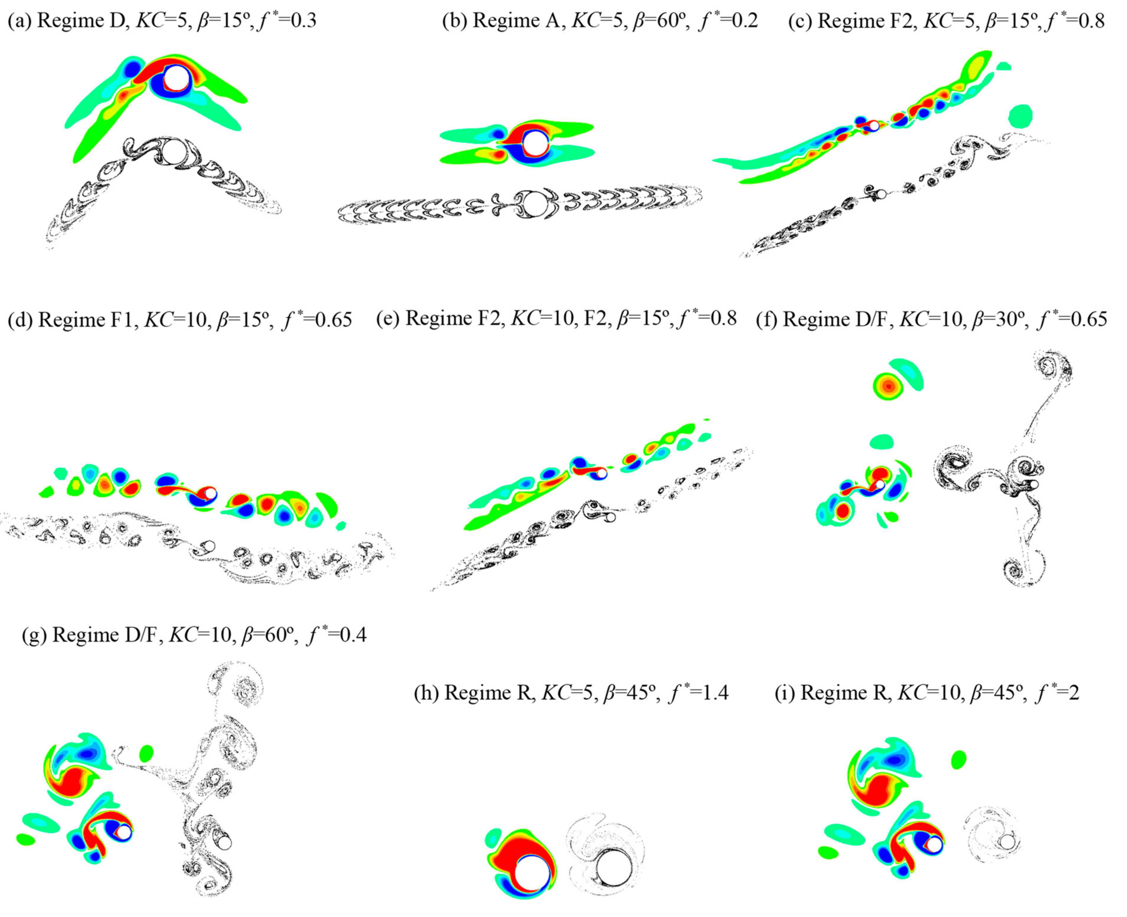
The vortex shedding regimes are further visualized by the streak lines together with the vorticity contours in Figure 12. Vorticity dissipates quickly in Regimes A and D, but the vortex streets can be identified using streak lines in Figure 12a,b. Regime D is a regime where vortices are only shed from one side of the cylinder, while Regime A is the regime where vortex shedding does not occur and the streak lines are in the form of two streams of particles going away from the cylinder from two opposite sides of the cylinder. Because the cylinder oscillates diagonally with a small amplitude, the vortex street in Figure 12b is slightly tilted. In Regime A, the vibration amplitude in the crossflow direction is very small, and as a result, the vortex pattern is similar to flow past a stationary cylinder at small KC number, as shown in Figure 12b. In Regimes F1 and F2, strong vortices are shed from the cylinder, and as a result, the two vortex streets identified by the vorticity contours are in the same pattern as the streak lines, as seen in Figure 12c–e. In Regime D/F, vortex shedding flow is aperiodic and the streak lines are in a pattern where fluid particles move away from the cylinder in three directions in Figure 12g and two directions in Figure 12 h. Because the vortex shedding pattern resembles Regime F sometimes and resembles Regime D sometimes, the pattern of the streak lines does not remain the same pattern. In regime R, the circulation of the vortices around the cylinder makes it difficult for the fluid particle to move away from the cylinder. The streak lines of Regime R are in a pattern where water particles also circle around the cylinder, as shown in Figure 12h,i.

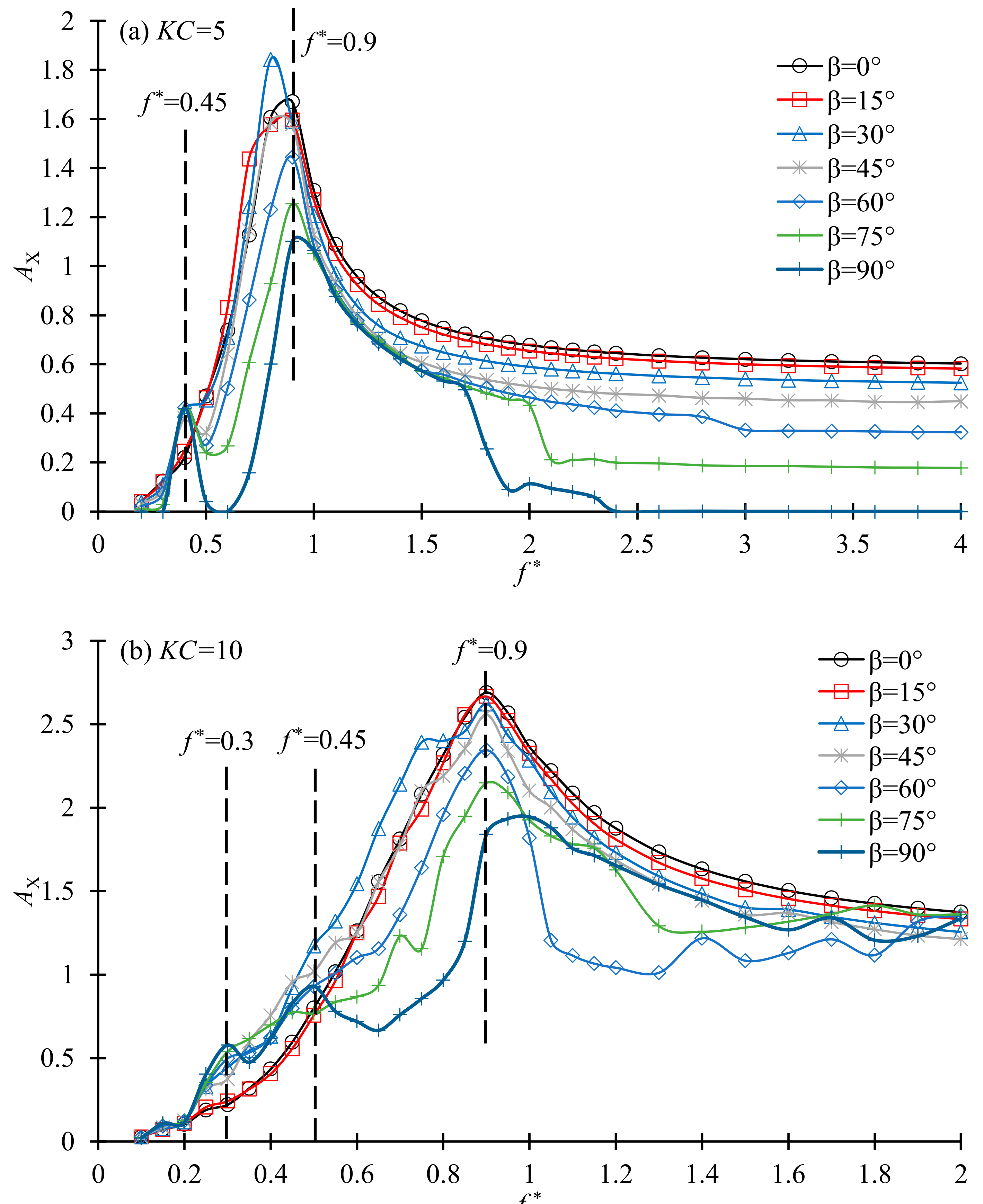
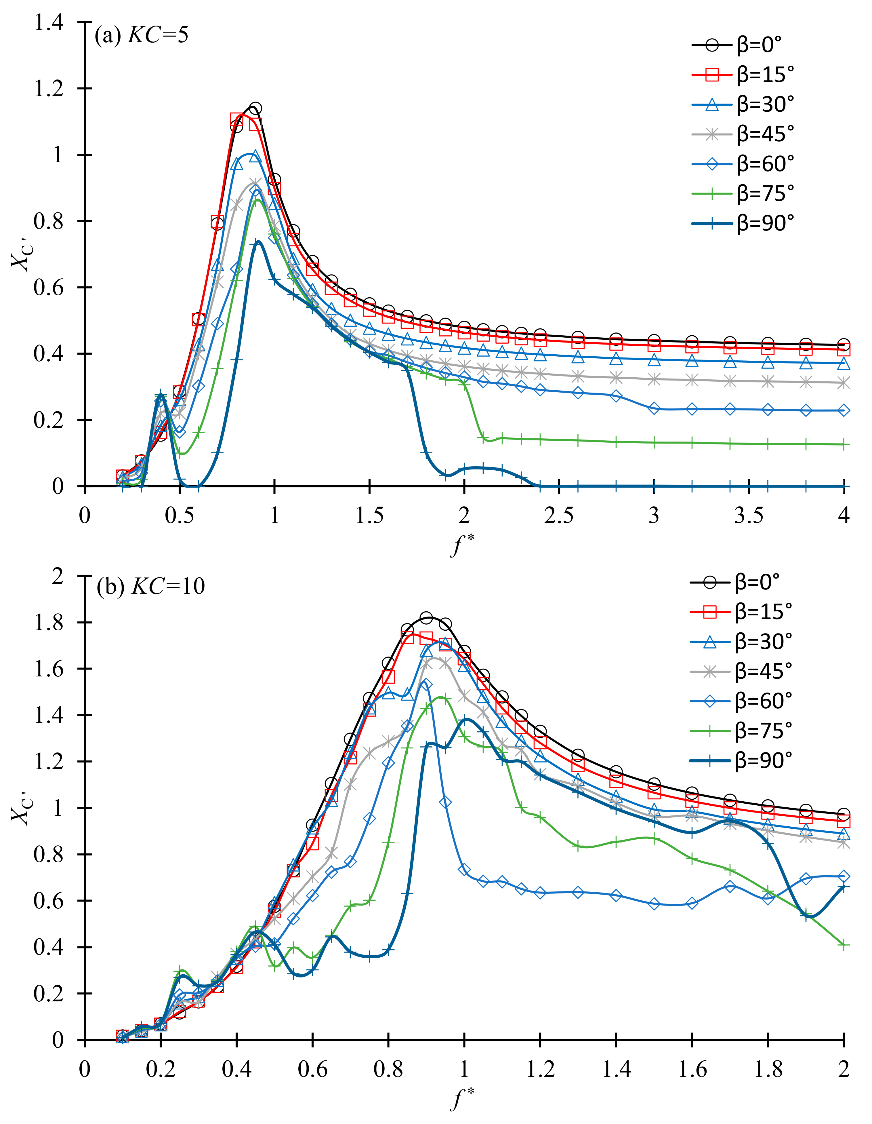
Figure 13 shows the variation of the vibration amplitude with the frequency ratio for KC = 5 and 10. The vibration amplitude is defined as $X_m=\max \left(\left|X\right|\right)$, where $\max \left(\left|X\right|\right)$ is the maximum displacement within one period. The maximum vibration amplitude within the last 100 periods is shown in Figure 13. The vibration amplitude is found to peak at about f ^* = 0.9 for all the values of β and both KC numbers. It peaks at a natural frequency ratio slightly smaller than 1 instead of 1 because of the effect of the added mass of the fluid. 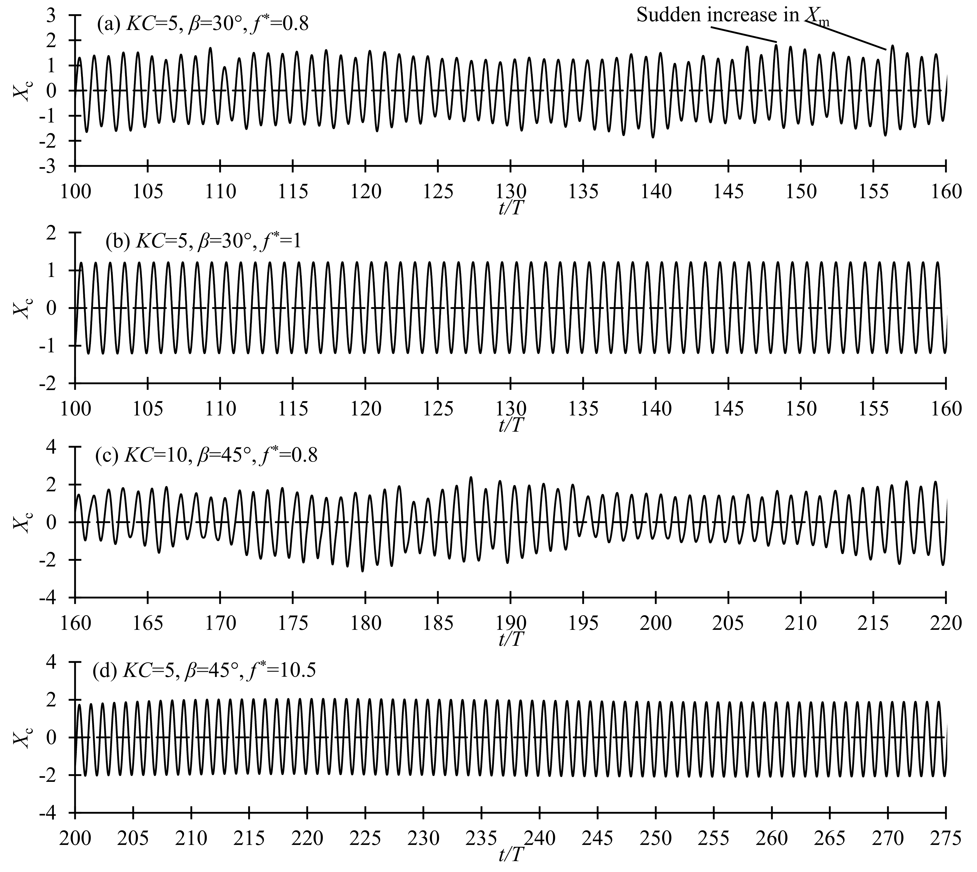The peak value of X_m reduces with the increase of β, except β = 30° and 15° for KC = 5 and 10, respectively. The time histories of the vibration shown in Figure 14 explain why the maximum vibration amplitude at β = 30° and 15° are higher than those of β = 0°. In Figure 14a, the vibration is irregular and occasionally vibration amplitude increases suddenly in one or two periods as indicated. Aperiodic force and vibration of cylinders in oscillatory flow at boundaries between flow regimes were also reported [15,39]. The occasional increase of the local X_m causes the abnormal increase in the X_m in Figure 13. In Figure 14c, the vibration is also irregular and X_m does not remain constant. The vibration time history becomes strongly aperiodic when the vibration is in Regime D/F and periodic when the vibration is in other regimes. The standard deviation of the vibration ($X_c^{’}$) shown in Figure 15 is obtained using 100 periods of data. $X_c^{’}$ is proportional to averaged amplitude of the vibration of all the 100 periods. It can be seen in Figure 15 that, generally, $X_c^{’}$ follows the same trend of X_m and the peak value of $X_c^{’}$ decreases with the decrease in β.

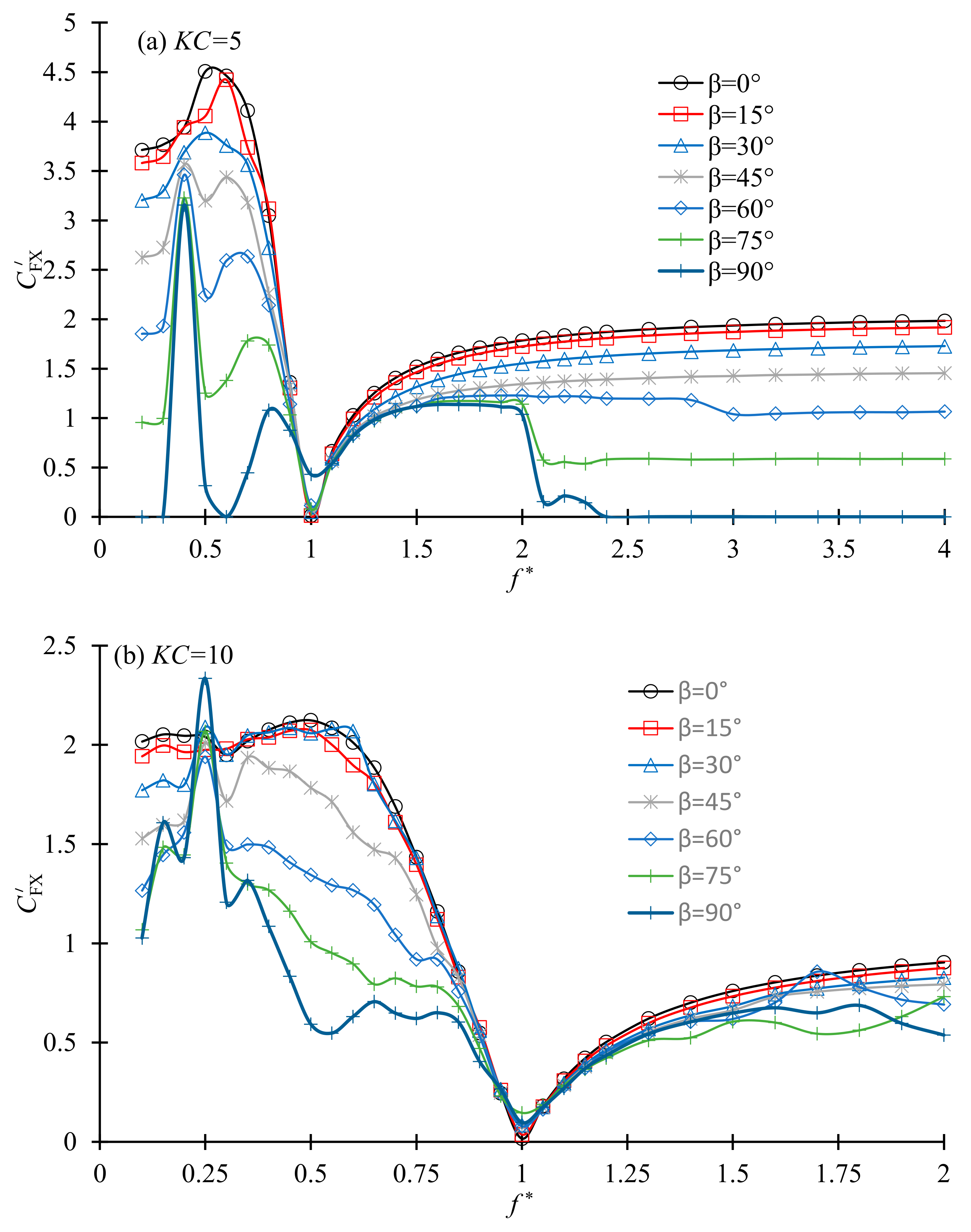
Figure 16 shows the variation of the standard deviation (SD) of the nondimensional force in the vibration direction of the cylinder with the natural frequency ratio. The nondimensional force is defined as $C_{\mathrm{FX}}=F_X/\left(D{U}_{\mathrm{m}}^2/2\right)$, where F_X is the dimensional force and the standard deviation (SD) of $C_{\mathrm{FX}}$ is represented as $C_{FX}^{’}$. The variation of X_m with $f^{*}$ in Figure 13 does not follow the trend of $C_{FX}^{’}$ because the frequency of the force plays a significant role in the vibration also, in addition to the magnitude of the force. The nondimensional force in the vibration direction reaches its minimum value at $f^{*}$ = 1 for both KC numbers. The sudden jump of the phase between the force and velocity in the x-direction can be seen in Figure 17. 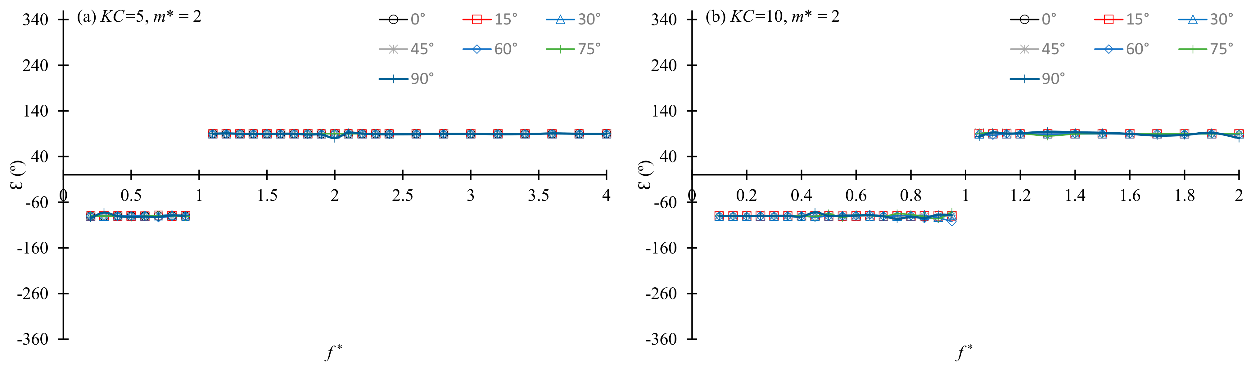When β is close to 90°, a maximum value of $C_{\mathrm{FX}}$ occurs at $f^{*}$ slightly smaller than 0.5 for KC = 5 and $f^{*}\approx$ 0.25 for KC = 10. Because the damping ratio is 0 in this study, there is not any net energy transferring between the fluid and the cylinder. This is the reason why the phase between the vibration velocity and the force is either −90° or 90°. The phase ε changes from −90° to 90° as $f^{*}$ exceeds 1 for all the vibration direction angles in Figure 17. Because the vibration amplitude in Figure 13 and the SD of force in Figure 17 are not correlated with each other, the degree of vibration cannot be purely estimated based on the magnitude of force.

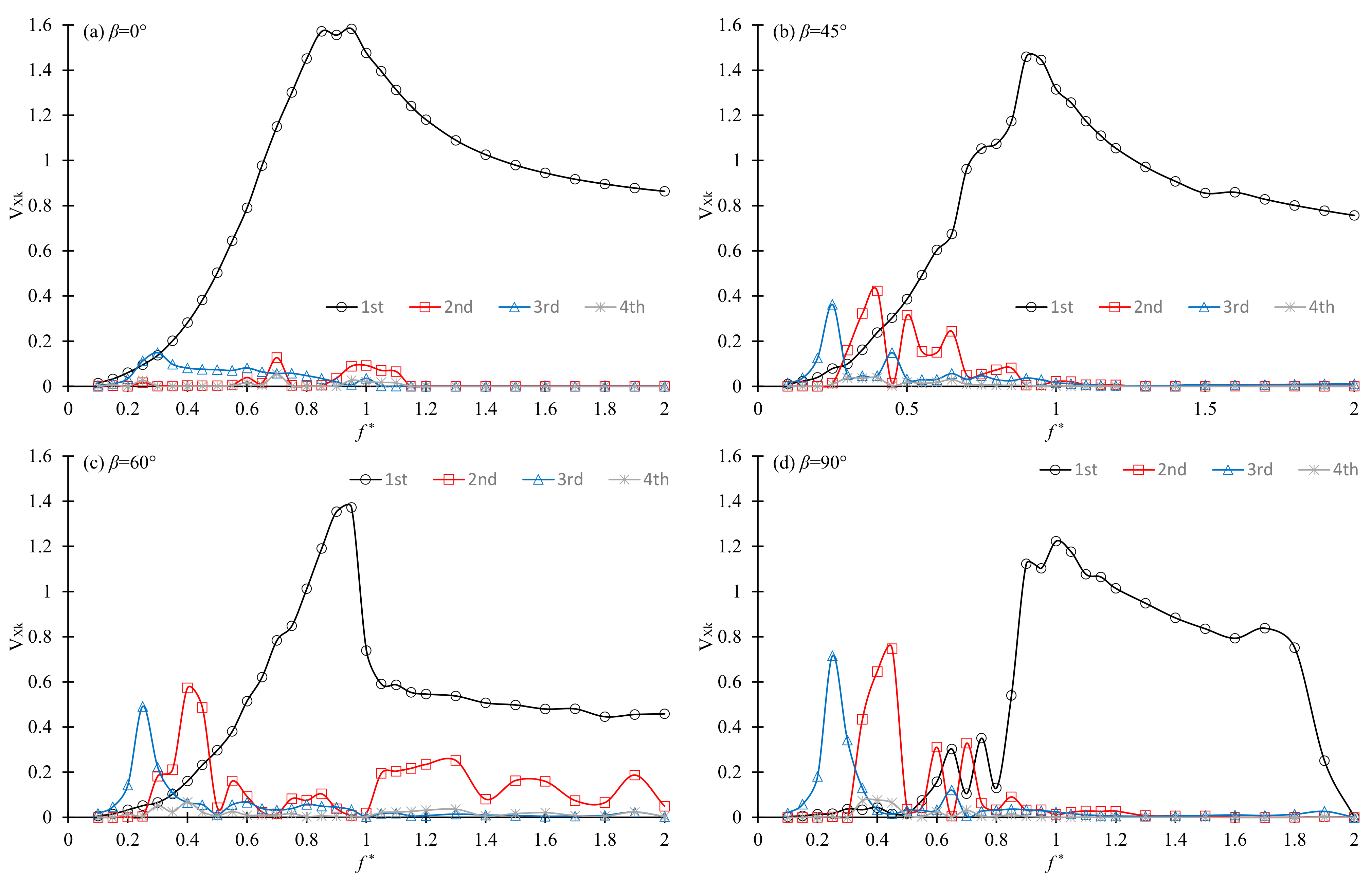
To understand the frequency component of the vibration, the nondimensional velocity of the cylinder in the x-direction is decomposed into harmonics as $V_X={\displaystyle \sum }_{k=1}^{\infty }{V}_{Xk}\sin \left(k\sigma t+{\phi }_k\right)$, where VX is the velocity of the cylinder in the x-direction, VXk is the amplitude of the k-th harmonic and φk is the phase of k-th harmonic. Figure 18 shows the variation of the first to fourth harmonics of the velocity of the cylinder with the frequency ratio for KC = 10. The contributions of the harmonics to the cylinder velocity are significantly affected by the vibration direction angle β. At β = 0°, VX is dominated by the first harmonic, as shown in Figure 18a, except $f^{*}\le 0.3$. Although third harmonic is comparable with at $f^{*}$ < 0.3, it does not excite strong vibration because its frequency is far different from the natural frequency. The contributions of the second and third harmonics increase and the contribution of the first harmonic decreases with the increase in β, especially at small values of $f^{*}$. At β = 60°, the dominance of second and third harmonics over the first harmonic can be clearly seen in the range of $f^{*}$ < 0.5 in Figure 18c. At β = 90° the contribution of the first harmonic is negligibly smaller than the second and third harmonics in the range of $f^{*}$< 0.5. The local maximum values near $f^{*}$ = 0.3 and 0.45 at β = 90° in Figure 13 are caused by the strong contributions of the second and third harmonics. At small values of β, the secondary local peaks in the vibration amplitude do not exist because the contributions of higher harmonics are too small to excite high amplitude vibration at high frequencies. Comparing Figure 16b with Figure 18 it can be seen that the force in the X-direction reaches its maximum at the $f^{*}$ values where the second harmonic of the VX peaks.

The dominance of higher-order harmonic forces at β = 45° to 90° and smaller frequency ratios can be explained by the flow patterns. At large values of β, the vibration is dominated by the fluid force in the crossflow direction. The fluid force in the crossflow direction is large when vortex shedding is strongly asymmetric, and its frequency is affected by the vortex shedding. From the regime map in Figure 10, the vortex shedding is dominated by Regime F or D/F as $f^{*}$ is less than 0.7. One and two pairs of vortices are shed from the cylinder within one period of flow in regime D and F, respectively. Considering the effect from the flow reversal, the frequency of the lift coefficient is twice or three-times the oscillatory flow frequency in Regimes D and F (one and two pairs vortex shedding in one period), respectively [21,40]. The higher-order lift coefficient in Regimes D and F are the reason for the higher-order vibration at small values of $f^{*}$ and β = 45° to 90°. The fluid force in the streamwise direction is dominated by the inertial force that is proportional to the acceleration with the frequency that is the same as the oscillatory flow frequency. That is the reason why the vibration in the streamwise direction is dominated by the first harmonic at β = 0°.

4. Conclusions

This paper examines the effect of the vibration direction of a vibrating cylinder in an oscillatory flow. Numerical simulations are conducted for Re = 150, m^* = 2, KC numbers KC = 5 and 10 and a wide range of vibration direction angles (0°, 15°, 30°, 45°, 60°, 75° and 90°).

In addition to the flow regimes that have been identified in the case where the cylinder is stationary, additional regimes are identified: Regime R, two variants of Regime F referred to as Regimes F1 and F2, respectively, and an unstable Regime D/F. In Regime R, a single, dominant large vortex circles continuously around the cylinder. It does not dissipate because it gains vorticity while it moves around the cylinder. While the vortex shedding patterns of Regimes F1 and F2 are the same as Regime F, their vortex street alignment angles are in the opposite and same directions of the vibration direction, respectively. In Regime D/F, the flow pattern resembles Regime F sometimes and Regime D sometimes. Regime D/F is unstable because the cylinder is attacked by the vortices frequently after the flow changes its direction.

All the identified flow regimes are mapped on the f ^*–β plan in Figure 3. The newly identified regime R is found to occupy large range of f ^* in the map. Regime D/F is only found at KC = 10. At β = 0° and 90°, Regimes F1 and F2 do not exist because the configuration is symmetric.

The maximum vibration amplitude occurs at $f^{*}\approx 0.9$, instead of 1, because of the effect of the added mass. This maximum vibration amplitude decreases with the increase in β. The second and third harmonics of the vibration displacement increase with the increase in vibration direction angle β in the low $f^{*}$ range. The dominance of the higher-order harmonics in Figure 18 leads to local maximum values at $f^{*}$= 0.4 and 0.25 in Figure 15a,b, respectively.