Lateral Buckling of Subsea Pipelines Triggered by Sleeper with a Nonlinear Pipe–Soil Interaction Model

Abstract

Buckle-initiation techniques, such as sleepers, are usually installed to trigger lateral buckling at pre-designated locations to release the axial compressive forces induced by thermal loading. Taking the nonlinear pipe–soil interaction model into account, a mathematical model is proposed to investigate the lateral buckling of subsea pipelines triggered by a sleeper. The numerical solution is validated by comparing the model with solutions in the literature, and the model shows good agreement. The discrepancy between them is analysed by presenting the effect of mobilisation distance during buckling. The influence of the breakout resistance, sleeper height, and sleeper friction coefficient on the buckled configuration, post-buckling behaviour, and minimum critical temperature difference is discussed parametrically. The results show that the deformation of the buckled pipeline shrinks, and both the minimum critical temperature difference and the maximum stress along the buckled pipeline enlarge when the nonlinear pipe–soil interaction model is incorporated. However, the influence of the nonlinear pipe–soil interaction reduces with increasing sleeper height.

1. Introduction

Subsea pipelines may buckle laterally due to the excessive axial compressive force due to high-temperature and high-pressure conditions. Lateral buckling occurs when the axial compressive force reaches critical levels. Lateral buckling, if not controlled, can lead to serious accidents involving local buckling, fracture, and fatigue [1]. To control this phenomenon, buckle initiation techniques, such as sleepers, are employed along pipelines to trigger buckles at predesigned locations. A sleeper is a pipe segment that is installed underneath and perpendicular to the pipeline, which typically has a low friction surface to reduce the lateral friction force. Thus, the pipeline is uplifted vertically. A combination of the vertical out-of-straightness and low lateral resistance results in reduced critical buckling force. When the sleeper is used as the buckle initiation facility, part of the pipeline is suspended. The pipeline segment at the end of the suspended section has a larger embedment into the seabed, since a vertical concentrated force exists. This embedment affects the lateral breakout resistance, which is a key design parameter governing the initiation of the lateral buckle. Thus, a nonlinear pipe–-soil interaction model is considered in the mathematical model to investigate the influence of breakout resistance on post-buckling behaviour.

The global buckling of subsea pipelines was investigated by numerous researchers. Hobbs’ solutions for a straight pipeline were derived by assuming specific buckling mode shapes and constant lateral soil resistance [2]. Based on this, an analytical model was proposed by Taylor and Gan [3] with a consideration of initial imperfection. A simplified analytical model was proposed by Croll [4] for upheaval buckling. The interaction between propagation buckling and global buckling in subsea pipelines was investigated by Karampour et al. [5]. This interaction leads to a significant reduction in buckle design capacity. The lateral buckling of imperfect pipelines was studied by Liu et al. [6], using FEM. The analytical solutions for the high-order lateral buckling of a pipeline with symmetric and anti-symmetric initial imperfection were derived by Hong et al. [7] and Liu et al. [8], respectively. Lateral buckling was investigated by Konuk [9,10] with coupled lateral and axial pipe–soil interactions. Zhang et al. [11,12] derived unified formulas for the critical buckling forces of the upheaval and lateral buckling of subsea pipelines with different types of initial imperfection. The influence of the pipe length on the lateral buckling behaviour of imperfect pipelines was investigated through FEM [13].

More recently, researchers investigated the influence of the nonlinear pipe–soil interaction model on lateral buckling. Zeng and Duan [14] used a quintic polynomial formula to simulate nonlinear pipe–soil interactions. Incorporating the tri-linear pipe–soil interaction model, Chee et al. [15] investigated the effect of imperfections on the buckling response through FEM. Considering both the initial imperfection and the nonlinear lateral soil resistance model, the critical force of the lateral buckling was analysed by assuming that the length of the buckled region equals the wavelength of initial imperfection [16].

To increase the reliability of buckle formation predictions, buckle initiation facilities were incorporated into the mathematical models. A single buoyancy or distributed buoyancy with a specific length installed along the pipeline was considered to derive some simple analytical solutions [17]. The critical load of lateral buckling triggered by a single buoyancy was investigated by Shi and Wang [18]. Moreover, dual distributed buoyancy sections with a gap between them were employed to initiate lateral buckling [19]. A new way to trigger lateral buckling is to introduce a pre-deformed section along the pipeline before installation [20]. Lateral buckling triggered by a sleeper was investigated experimentally by Silva-Junior et al. [21] and de Oliveira Cardoso and Solano [22]. Bai et al. [23] studied the lateral buckling triggered by dual sleepers through FEM. Analytical solutions for antisymmetric buckling modes triggered by a sleeper were obtained by Wang and Tang [24]. They found that the symmetric buckling mode was more likely to occur with lower sleeper friction or smaller sleeper height. Hong and Liu [25] investigated the vertical deflection of a pipeline on a sleeper by FEM.

By assuming constant lateral soil resistance, analytical solutions were derived for the lateral thermal buckling triggered by a sleeper in [26]. In practice, the pipeline always has an initial embedment into the soil and the lateral soil resistance is not constant. However, there are no studies about lateral thermal buckling triggered by sleepers that consider nonlinear lateral soil resistance.

The innovative aspect of this study is the nonlinear pipe–soil interaction model that is incorporated into the governing equations. In previous published studies about lateral buckling triggered by sleepers, the lateral soil resistance, $f\left(w_2\right)$, is assumed to be constant. However, in this study, this function is nonlinear and it includes the effect of breakout resistance. This is due to the fact that in practice, pipe–soil interactions are nonlinear.

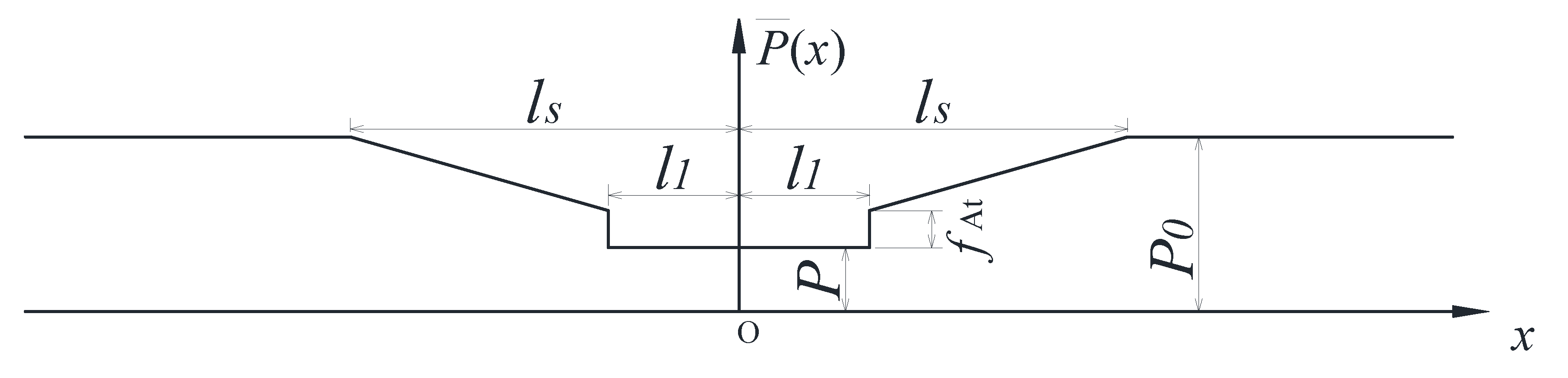
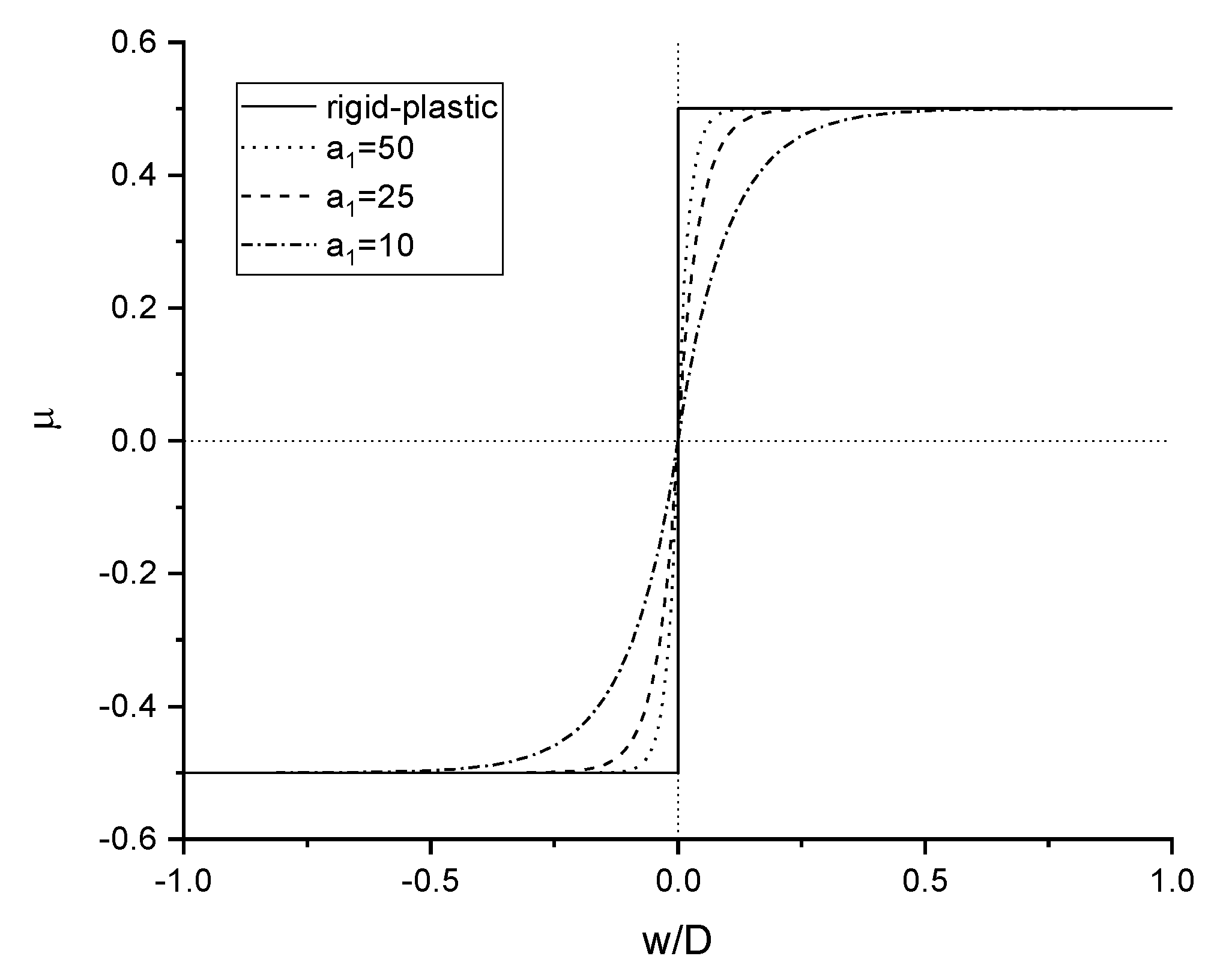
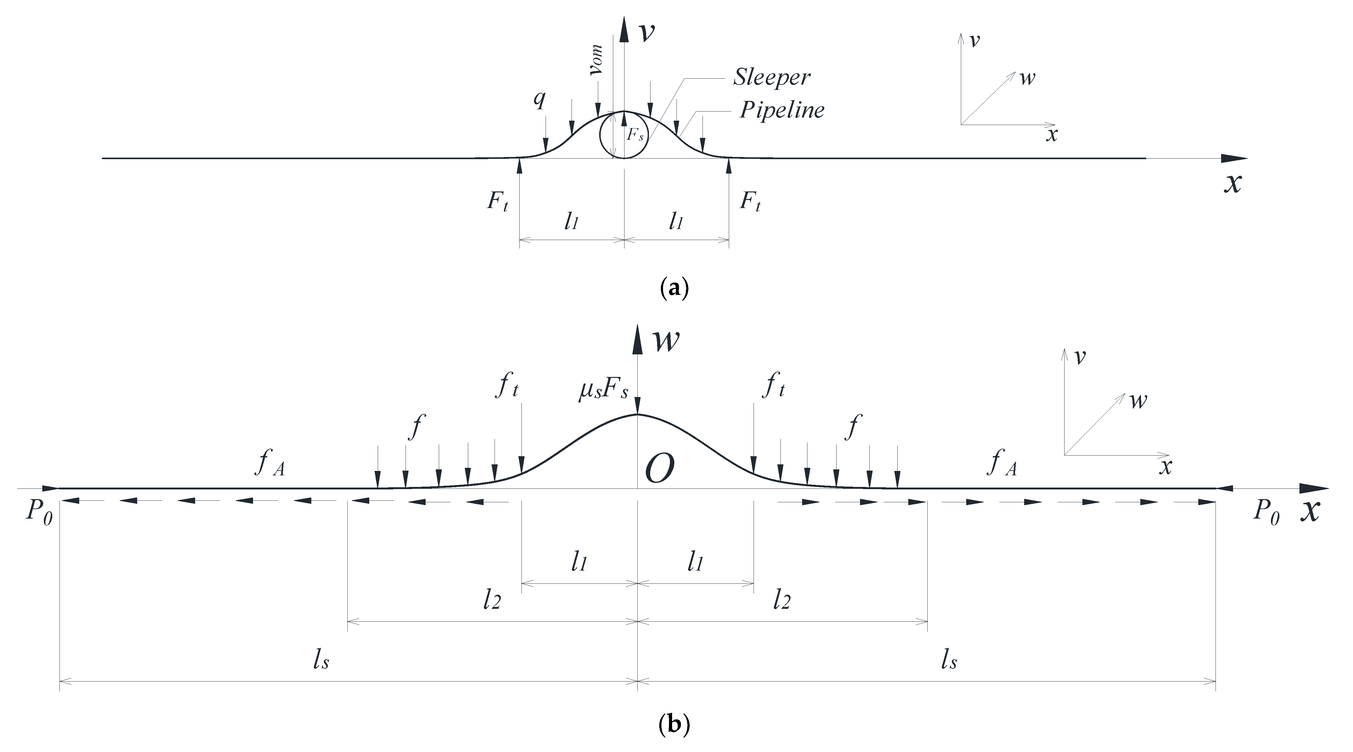
2. Mathematical Modelling

To avoid rogue buckles along subsea pipelines, buckle-initiation techniques, such as installing sleepers along the pipeline, are usually employed to trigger the pipeline to buckle in a controlled way at the predesignated location. For a pipeline laid on a sleeper and subjected to a temperature difference $T_0$, the axial compressive force is accumulated. The axial compressive force, $P_0$, is expressed as

$$P_0=EA\alpha T_0$$

(1)

where $E$ is the elastic modulus, $A$ is the cross-sectional area of the pipeline, and $\alpha$ is the coefficient of linear thermal expansion.

When $P_0$ is larger than the critical value, lateral buckling can be triggered at sleeper. The configuration and load distribution of lateral buckling are illustrated in Figure 1. From Figure 1a, it is clear that part of the pipe segment within $-l_1\le x\le l_1$ is uplifted by the sleeper. In $-l_1\le x\le l_1$, the soil resistances are zero. However, there are concentrated contact forces $F_s$ between pipeline and sleeper at the sleeper and $F_t$ between the pipe and seabed at the end of the suspended section, respectively. The vertical configuration of the pipeline laid on a sleeper was solved by Wang et al. [26]. From their derivation, $F_s$ and $F_t$ can be expressed as

$$F_s=\frac{4}{3}{W}_{pipe}{l}_1 \mathrm{and} F_t=\frac{1}{3}{W}_{pipe}{l}_1$$

(2)

where $W_{pipe}$ is the submerged weight per unit length and $l_1$ is the half-length of the free span, solved by

$$l_1=\sqrt[4]{\frac{72EI{v}_{om}}{W_{pipe}}}$$

(3)

where $I$ is the moment of inertia and $v_{om}$ is the sleeper height. Therefore, the value of $l_1$ can be obtained by Equation (3) when $v_{om}$ is specified. Furthermore, $F_s$ and $F_t$ can be solved.

After the pipeline buckles, additional pipe coming from the thermal expansion is fed into the buckled section. Therefore, the axial force reduces partially due to the release of axial strain (see Figure 2). The axial force within the suspended region $-l_1<x<l_1$, denoted by $P$, is constant. At $x=\pm l_1$, there is a jump in axial force with an amplitude of $f_{At}$ induced by $F_t$. Within the region where the pipeline makes contact with the seabed, the axial force increases because of the restraint of axial soil resistance. The axial force will reach $P_0$ at $x=\pm l_s$. From Figure 2, the axial force distribution $\overline{P}\left(x\right)$ is

$$\overline{P}\left(x\right)=\{\begin{array}{l}P \left(0\le x<l_1\right)\\ P+f_{At}+f_A\left(x-l_1\right) \left(l_1\le x\le l_s\right)\end{array}$$

(4)

where $f_A={\mu }_A{W}_{pipe}$ is the axial soil resistance per unit length and ${\mu }_A$ is the axial friction coefficient. The force $f_{At}={\mu }_A{F}_t$ is induced by $F_t$.

The axial force at $x=l_s$ is

$$\overline{P}\left(l_s\right)=P_0=P+f_{At}+f_A\left(l_s-l_1\right)$$

(5)

Linear beam theory is used to simulate pipeline buckling. Thus, the equilibrium equations governing lateral deformation are [27]:

$$\{\begin{array}{l}EI\frac{d^4{w}_1}{d{x}^4}+P\frac{d^2{w}_1}{d{x}^2}=0 \left(0\le x<l_1\right)\\ EI\frac{d^4{w}_2}{d{x}^4}+\overline{P}\left(x\right)\frac{d^2{w}_2}{d{x}^2}=-f\left(w_2\right) \left(l_1\le x\le l_2\right)\end{array}$$

(6)

where $w_1$ and $w_2$ are lateral deflections, $EI$ is bending stiffness, and $f\left(w_2\right)$ is the nonlinear lateral soil resistance determined by the nonlinear pipe–soil interaction model, as shown in Figure 3. Here, the variation in the axial force within the buckled region $l_1\le x\le l_2$ is ignored when solving lateral deformations. This assumption is acceptable [26,28].

Here, the nonlinear pipe–soil interaction model proposed by Chatterjee et al. [29] is employed. It can simulate breakout resistance and is given by

$$\mu =\frac{w}{\left|w\right|}\left({\mu }_{brk}\left(1-{\mathrm{e}}^{-a_1{\left(\frac{\left|w\right|}{D}\right)}^{a_2}}\right)+\left({\mu }_{res}-{\mu }_{brk}\right)\left(1-{\mathrm{e}}^{-a_3{\left(\frac{\left|w\right|}{D}\right)}^{a_4}}\right)\right)$$

(7)

where $\mu$, ${\mu }_{brk}$ and ${\mu }_{res}$ are the equivalent friction coefficients, and $D$ is the external diameter of the pipeline. The quantities $f\left(w\right)=\mu W_{pipe}$, $F_{brk}={\mu }_{brk}{W}_{pipe}$ and $F_{res}={\mu }_{res}{W}_{pipe}$ are, therefore, respectively, the nonlinear lateral soil resistance, the breakout resistance, and the residual resistance. The value of the coefficient $a_3$ in [29] is given as

$$a_3=a_5\left(\frac{W_{pipe}}{V_{max}}\right)+a_6$$

(8)

where $W_{pipe}$ is the weight of the pipe and $V_{max}$ is the vertical bearing capacity. The values of $a_5$ and $a_6$ are calculated by

$$a_5=8.2\frac{v_{init}}{D}-4.9, a_6=-5.8\frac{v_{init}}{D}+4.5$$

(9)

where $v_{init}$ is the initial embedment of the pipe into the soil. In [29], $a_1=25$ and $a_4=1.5$ are employed, but $a_2=1$ is used here in order to have a finite linear resistance, which is physically realistic. $V_{max}=5W_{pipe}$ and $v_{init}=0.3\mathrm{D}$ are adopted so that $a_3=2.272$, and set ${\mu }_{res}=$0.5.

Due to symmetry, half a pipeline is considered. The slope of the deflection at $x=0$ is zero, while the shear force $f_{ow}={\mu }_s{F}_s/2$ at $x=0$ is induced by the friction force ${\mu }_s{F}_s$. Here, ${\mu }_s$ is the friction coefficient between pipeline and sleeper. The displacement, slope, and moment at $x=l_2$ are also zero. The boundary conditions at $x=0$ and $x=l_2$ are

$$\{\begin{array}{l}\frac{d{w}_1}{dx}\left(0\right)=0\\ \frac{d^3{w}_1}{d{x}^3}\left(0\right)+\frac{f_{ow}}{EI}=0\\ w_2\left(l_2\right)=0\\ \frac{d{w}_2}{dx}\left(l_2\right)=0\\ \frac{d^2{w}_2}{d{x}^2}\left(l_2\right)=0\end{array}$$

(10)

The displacement, slope, and bending moment must be continuous at the touchdown point $x=l_1$, while there is a jump in shear force with an amplitude of $f_t={\mu }_{res}{F}_t$ at $x=l_1$ induced by the force $F_t$. Thus, additional conditions at $x=l_1$ are

$$\{\begin{array}{l}{w}_1\left(l_1\right)=w_2\left(l_1\right)\\ \frac{d{w}_1}{dx}\left(l_1\right)=\frac{d{w}_2}{dx}\left(l_1\right)\\ \frac{d^2{w}_1}{d{x}^2}\left(l_1\right)=\frac{d^2{w}_2}{d{x}^2}\left(l_1\right)\\ \frac{d^3{w}_1}{d{x}^3}\left(l_1\right)=\frac{d^3{w}_2}{d{x}^3}\left(l_1\right)+\frac{f_t}{EI}\end{array}$$

(11)

With Equations (10) and (11), the nonlinear governing equations are solved numerically by the shooting method [30]. Once the lateral deflections are known, the geometric shortening $u_2$ is obtained by

$$u_2=\frac{1}{2}{{\displaystyle \int }}_0^{l_1}{\left(\frac{d{w}_1}{dx}\right)}^{2}dx+\frac{1}{2}{{\displaystyle \int }}_{l_1}^{l_2}{\left(\frac{d{w}_2}{dx}\right)}^{2}dx$$

(12)

The following compatibility condition is employed to link the lateral deflection and the thermal loading induced deflection:

$$u_1=u_2$$

(13)

where $u_1$ is thermal expansion in $0<x<l_s$.

We have

$$u_1={{\displaystyle \int }}_0^{l_s}\frac{\Delta \overline{P}\left(x\right)}{EA}dx$$

(14)

where $\Delta \overline{P}\left(x\right)=P_0-\overline{P}\left(x\right)$.

Thus, this leads to

$$u_1=\frac{f_A{\left(l_s-l_1\right)}^2}{2EA}+\frac{\left(P_0-P\right)l_1}{EA}$$

(15)

The following formula is obtained by combining Equations (5), (13), and (15).

$$l_s=\sqrt{\frac{1}{3}{l}_1^2+\frac{2EA{u}_2}{f_A}}$$

(16)

With Equations (5) and (16), one finally obtains

$$P_0=P+f_A\left(\sqrt{\frac{1}{3}{l}_1^2+\frac{2EA{u}_2}{f_A}}-\frac{2}{3}{l}_1\right)$$

(17)

The bending moment is obtained by

$$M=EI\frac{d^{2}w}{d{x}^2}$$

(18)

where $w$ stands for $w_1$ or $w_2$, and the bending stress ${\sigma }_M$ is

$${\sigma }_M=\frac{MD}{2I}$$

(19)

The maximum stress is

$${\sigma }_m={\sigma }_P+{\sigma }_{Mm}$$

(20)

where the stresses ${\sigma }_P$ and ${\sigma }_{Mm}$, induced by axial force $P$ and maximum bending moment $M_m$, respectively, are

$$\{\begin{array}{l}{\sigma }_P=\frac{P}{A}\\ {\sigma }_{Mm}=\left|\frac{M_{m}D}{2I}\right|\end{array}$$

(21)

3. Results

The mathematical model is validated by comparing it with the analytical solution in [26], and the discrepancy between them is discussed. Next, the influence of ${\mu }_{brk}$, $v_{om}$ and ${\mu }_s$ is analysed. The results are obtained by employing the analytical formulation developed in Section 2 and taking the parameters in

Table 1. Parameters.

Parameter	Value	Unit
External diameter $D$	323.9	mm
Wall thickness $t$	12.7	mm
Elastic modulus $E$	206	GPa
Steel density $\rho$	7850	$\mathrm{kg}/{\mathrm{m}}^3$
Coefficient of thermal expansion $\alpha$	$1.1\times {10}^{-5}$	$°\mathrm{C}$
Axial friction coefficient ${\mu }_A$	0.5	---

.

One should note that only the analytical solutions in Figure 4 and Figure 5 come from [26], which is used to validate the numerical results obtained in this study. In [26], the lateral soil resistance is assumed to be constant, while in the present study, nonlinear lateral soil resistance is considered. Moreover, in [26], analytical solutions are obtained due to the assumption of constant lateral soil resistance. In the present study, because the lateral soil resistance is nonlinear, Equation (6) cannot be solved analytically. Thus, the shooting method is used to solve Equation (6) to obtain the numerical results.

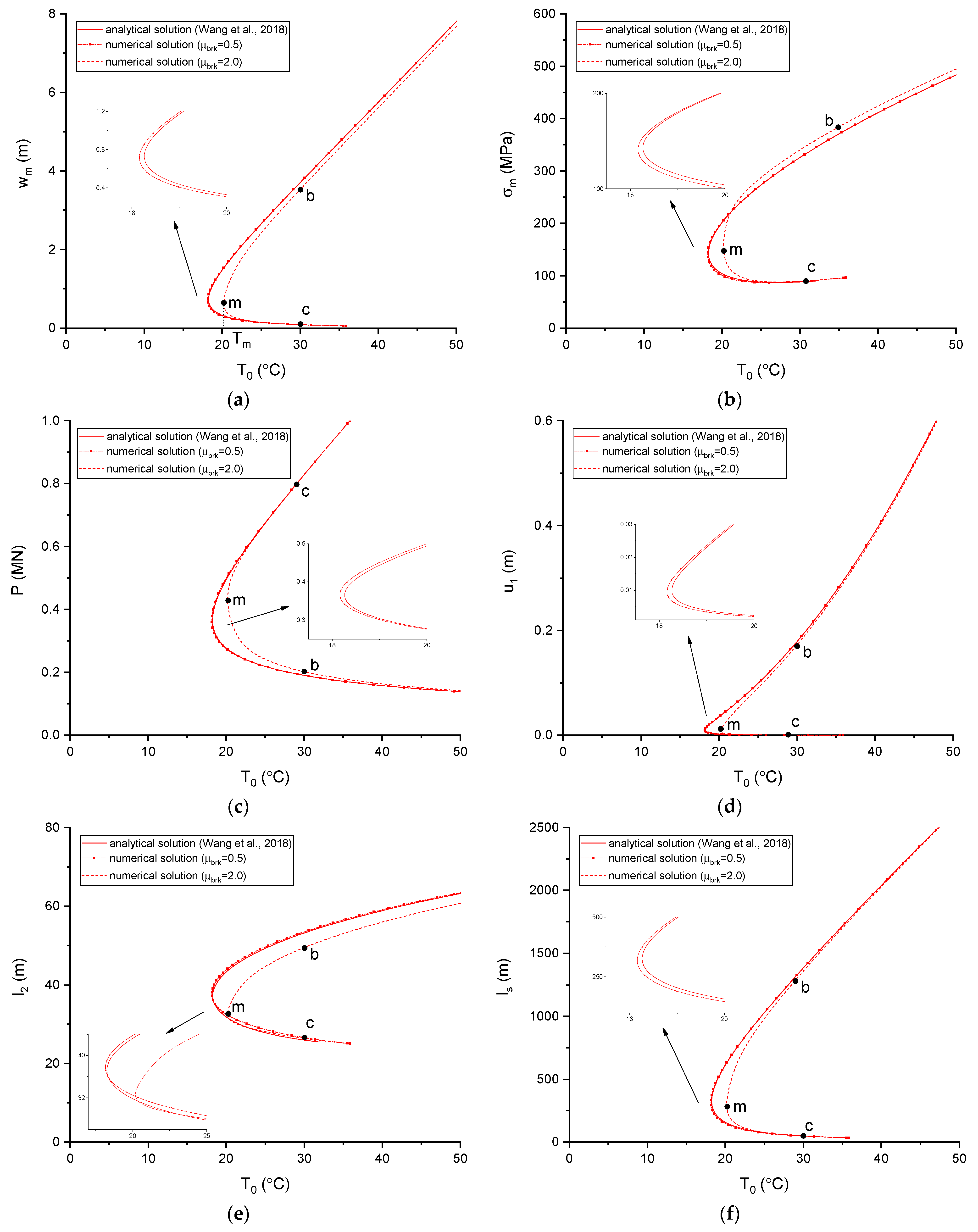
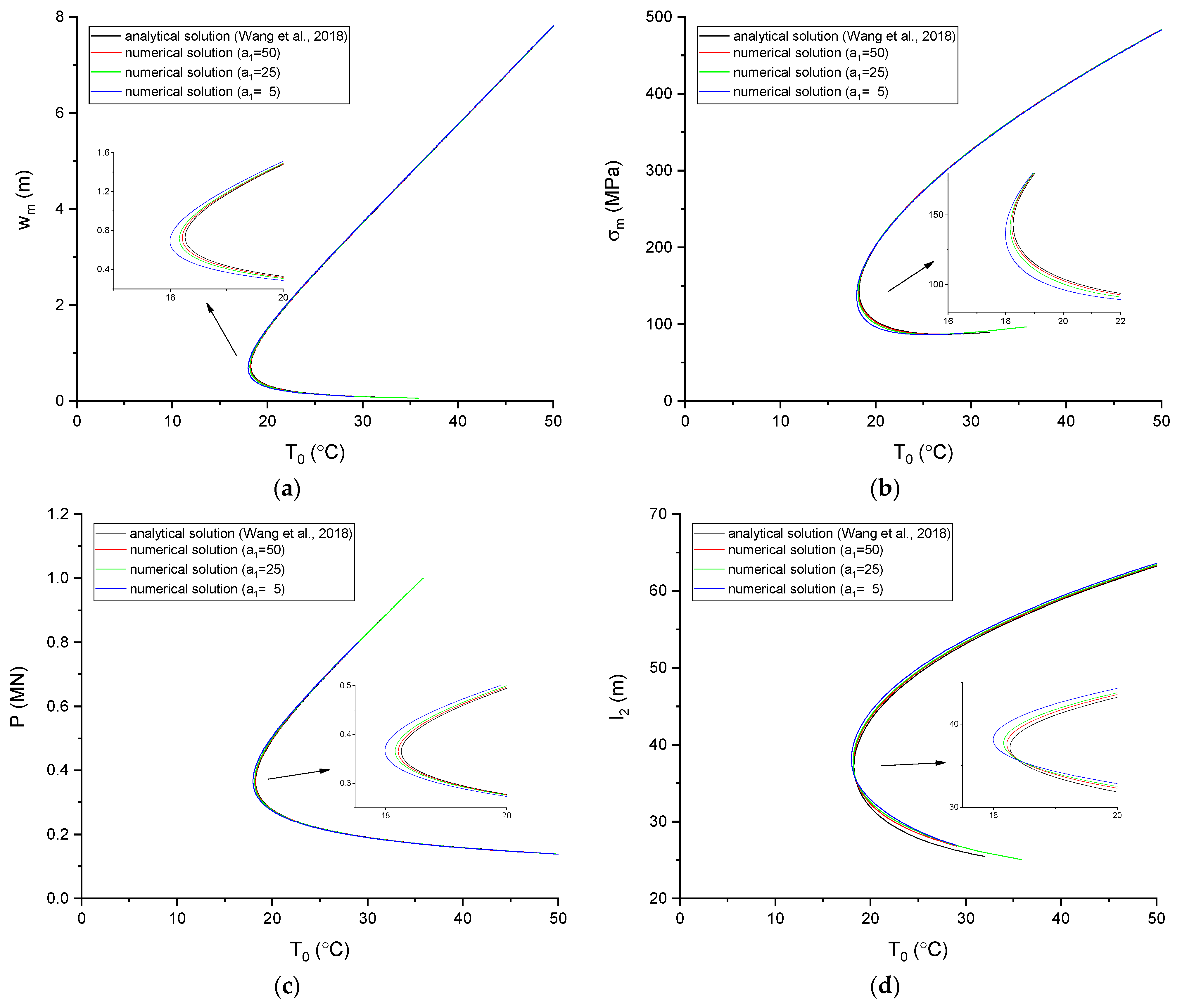
3.1. Validation

The solutions obtained in this study were validated by comparing them with the analytical solutions in [26], as shown in Figure 4. An error analysis is shown in Figure 5. In Figure 4, the analytical solutions are obtained by using the formulas derived in Wang et al. [26] with constant lateral soil resistance. To compare with the analytical solutions, the numerical solutions shown in Figure 4 are obtained by assuming ${\mu }_{brk}=0.5$. For ${\mu }_{brk}=0.5$, the nonlinear pipe–soil interaction model is reduced to elastic-plastic (see Figure 3). The numerical solutions for ${\mu }_{brk}=2.0$ are also illustrated in Figure 4 to show the influence of the nonlinear pipe–soil interaction.

In Figure 4, there are two branches for each solution, which are denoted as m-b and m-c. The temperature difference at m, i.e., $T_m$, is called the minimum critical temperature difference, since solutions only exist for $T_0>T_m$.

From Figure 4, the numerical solutions for ${\mu }_{brk}=0.5$ are in good agreement with the analytical solutions, except that there is a slight discrepancy between them around $T_m$. This discrepancy comes from the difference in mobilization distance. For the rigid-plastic model, the resistance is always constant (see Figure 3). For the elastic-plastic model, the lateral soil resistance increases from zero to residual resistance gradually (see Figure 3).

In Figure 4, the discrepancy between the analytical and numerical solutions reduces as the temperature difference increases. The reason for this is that the displacement amplitude increases along with the temperature difference, so that more pipe sections fall into the region of constant lateral soil resistance for numerical solutions.

A more detailed error analysis is illustrated in Figure 5. Figure 6 shows that the mobilization distance is controlled by the parameter $a_1$. The mobilization distance is the distance that the lateral resistance reaches ${\mu }_{brk}$. In Figure 6, ${\mu }_{brk}={\mu }_{res}=0.5$, so the mobilization distance in Figure 6 is the distance at which $\mu$ reaches 0.5. The elastic-plastic model approaches the rigid-plastic model for larger $a_1$, since the mobilization distance becomes smaller. In Figure 5, the discrepancy between the analytical and numerical solutions becomes smaller for larger $a_1$. In Figure 4 and Figure 5, the discrepancy in half-buckled length $l_2$ is larger than in the other parameters. This is because the deflection at the ends of the buckled section is small, and it is affected by the mobilization distance. For the remaining parameters, the discrepancy between the analytical and numerical solutions is small enough.

In Figure 4a, $T_m$ becomes larger when the nonlinear pipe–-soil interaction model is considered, which means that lateral buckling can only be triggered at higher temperature differences. At the same temperature difference, both $w_m$ and $l_2$ become smaller when considering the nonlinear pipe–soil interaction model (see Figure 4a,e). Thus, the use of an additional pipe to create lateral deflection, which comes from thermal expansion, also reduces (see Figure 4d), so that $l_s$ decreases, as shown in Figure 4f. However, $P$ within the buckled section becomes larger due to the restriction of the breakout resistance. Moreover, at the same temperature difference, the maximum stress ${\sigma }_m$ becomes larger when nonlinear pipe–soil interaction is considered. This means that the maximum stress is underestimated when assuming the lateral soil resistance to be constant.

3.2. Parametric Study

3.2.1. Influence of ${\mu }_{brk}$

The influence of ${\mu }_{brk}$ on the buckled configuration, post-buckling behaviour, and minimum critical temperature difference $T_m$ is shown in Figure 7, Figure 8 and Figure 9, respectively.

In Figure 7, the dashed curves are the pipe sections in contact with the seabed, and the solid curves are the pipe sections suspended due to the existence of the sleeper. In Figure 7a, both the touchdown and suspended pipe segments shrink with larger ${\mu }_{brk}$. In Figure 7b, there are two extrema of bending stress in the positive direction. Another three extrema of bending stress occur around the sleeper. One local minimum (absolute value) of bending stress appears at the sleeper, while there are two other local maxima (absolute value) of bending stress close to the sleeper. The occurrence of the local minimum (absolute value) of bending stress at the sleeper is induced by the friction force between the pipeline and the sleeper. For each specific ${\mu }_{brk}$, the maximum bending stress is located at the local maxima (absolute value) of bending stress close to the sleeper. For larger ${\mu }_{brk}$, all the extrema of bending stress in both positive and negative directions become larger.

In Figure 8a, $T_m$ is larger for larger ${\mu }_{brk}$. A more detailed analysis on the influence of ${\mu }_{brk}$ on $T_m$ is shown in Figure 9, which shows that $T_m$ increases with increasing ${\mu }_{brk}$ for specific values of $v_{om}$ and ${\mu }_s$, and the increasing rate of $T_m$ reduces with the increase in ${\mu }_{brk}$. In Figure 9a, under the same ${\mu }_{brk}$, $T_m$ is larger for smaller $v_{om}$. The increasing rate of $T_m$ with increasing ${\mu }_{brk}$ is also larger for smaller $v_{om}$. The reason is that since there are less length of suspended pipeline and larger length of touchdown pipeline with the smaller $v_{om}$, the breakout resistance has a larger influence on the initiation of lateral buckling. In Figure 9b, under the same ${\mu }_{brk}$, $T_m$ becomes larger for larger ${\mu }_s$. The increase in the rate of $T_m$ along with the increasing ${\mu }_{brk}$ remains almost the same for different values of ${\mu }_s$. The reason for this is that the friction force between the pipeline and the sleeper becomes larger for larger ${\mu }_s$; however, the value of ${\mu }_s$ has no influence on the lengths of the suspended or touchdown pipeline segments.

In Figure 8a,e, both the displacement amplitude $w_m$ and the half-buckled length $l_2$ increase with the increasing $T_0$, and need more thermal expansion $u_1$ to form the buckled deflection (see Figure 8d). Thus, larger $l_s$ is required for larger $T_0$, as shown in Figure 8f. The maximum stress also increases with increasing $T_0$ (see Figure 8b) since large deflection occurs; however, the axial force $P$ reduces with increasing $T_0$ (see Figure 8c).

In Figure 8a,e, at a specific temperature difference, both $w_m$ and $l_2$ become smaller for larger ${\mu }_{brk}$. The reason for this is that since the breakout resistance is larger for larger ${\mu }_{brk}$, the pipeline is subjected to greater lateral soil resistance. The deflection shrinks with larger ${\mu }_{brk}$, as shown in Figure 7a. Therefore, both $u_1$ and $l_s$ become smaller with larger ${\mu }_{brk}$ at the same temperature difference (see Figure 8d,f).

However, $P$ becomes larger with larger ${\mu }_{brk}$ (see Figure 8c). The reason for this is that the reduction in the axial force reduces, since the greater breakout resistance restricts the deflection of the buckled pipeline. Moreover, ${\sigma }_m$ along the buckled pipeline becomes larger for larger ${\mu }_{brk}$ (see Figure 8b). After considering the nonlinear pipe–soil interaction model, both $T_m$ and ${\sigma }_m$ in the pipeline became larger. When the nonlinear pipe–soil interaction model is not included, lateral buckling may fail to be triggered by the sleeper, and the maximum stress along the buckled pipeline may exceed the allowable stress in the design.

3.2.2. Influence of $v_{om}$

The influence of $v_{om}$ on the buckled configuration, post-buckling behaviour, and minimum critical temperature difference $T_m$ are shown in Figure 10, Figure 11 and Figure 12, respectively.

From Figure 10a, it is clear that the length of the suspended pipe segment becomes larger with larger sleeper heights, $v_{om}$. The deflection of the buckled pipeline enlarges with larger $v_{om}$. Because the soil resistance for the suspended pipeline is zero, the buckled pipeline has less restriction from the seabed foundation with larger $v_{om}$. The deflection of the buckled pipeline enlarges with larger $v_{om}$, but both the local minimum and the local maximum (absolute value) of the bending stress become smaller with larger $v_{om}$, as shown in Figure 10b. This is because the deflection of the buckled pipeline is more benign with larger $v_{om}$.

In Figure 11a, $T_m$ becomes smaller with larger $v_{om}$. Figure 12 illustrates the influence of $v_{om}$ on $T_m$ in detail. In Figure 12, $T_m$ decreases with increasing $v_{om}$ for specific values of ${\mu }_{brk}$ and ${\mu }_s$, and the decreasing rate of $T_m$ reduces with increasing $v_{om}$. In Figure 12a, under the same $v_{om}$, $T_m$ becomes larger for larger ${\mu }_{brk}$. The influence of ${\mu }_{brk}$ on $T_m$ becomes smaller for larger $v_{om}$, since the length of suspended pipeline with zero soil resistance is greater. In Figure 12b, under the same $v_{om}$, $T_m$ is larger with larger ${\mu }_s$. The decreasing rate of $T_m$ with increasing $v_{om}$ becomes smaller with larger ${\mu }_s$. The influence of ${\mu }_s$ on $T_m$ is larger with larger $v_{om}$. The reason for this is that the concentrated contact force between the pipeline and the sleeper becomes larger with larger $v_{om}$, so that the friction force between the pipeline and the sleeper becomes larger with larger $v_{om}$. Therefore, an effective way to reduce $T_m$ is to increase the sleeper height $v_{om}$; however, the corresponding weakness is that the suspended pipeline will be longer, which may lead to vortex-induced vibration.

In Figure 11a,e, at a specific temperature difference, both $w_m$ and $l_2$ become larger with larger $v_{om}$. This is because the length of the suspended pipeline with zero soil resistance increases with increasing $v_{om}$, as shown in Figure 10a. There is less restriction from the seabed foundation with larger $v_{om}$. Due to the larger deflection with larger $v_{om}$, the requirement of additional pipes to feed into the buckled section increases, which creates the need for more thermal expansion (see Figure 11d) and a longer feed-in region (see Figure 11f). The axial force $P$ becomes smaller with larger $v_{om}$, since a larger deflection occurs to release more axial force, as shown in Figure 11c. The maximum stress ${\sigma }_m$ along the buckled pipeline reduces with larger ${\mu }_{brk}$ (see Figure 11b).

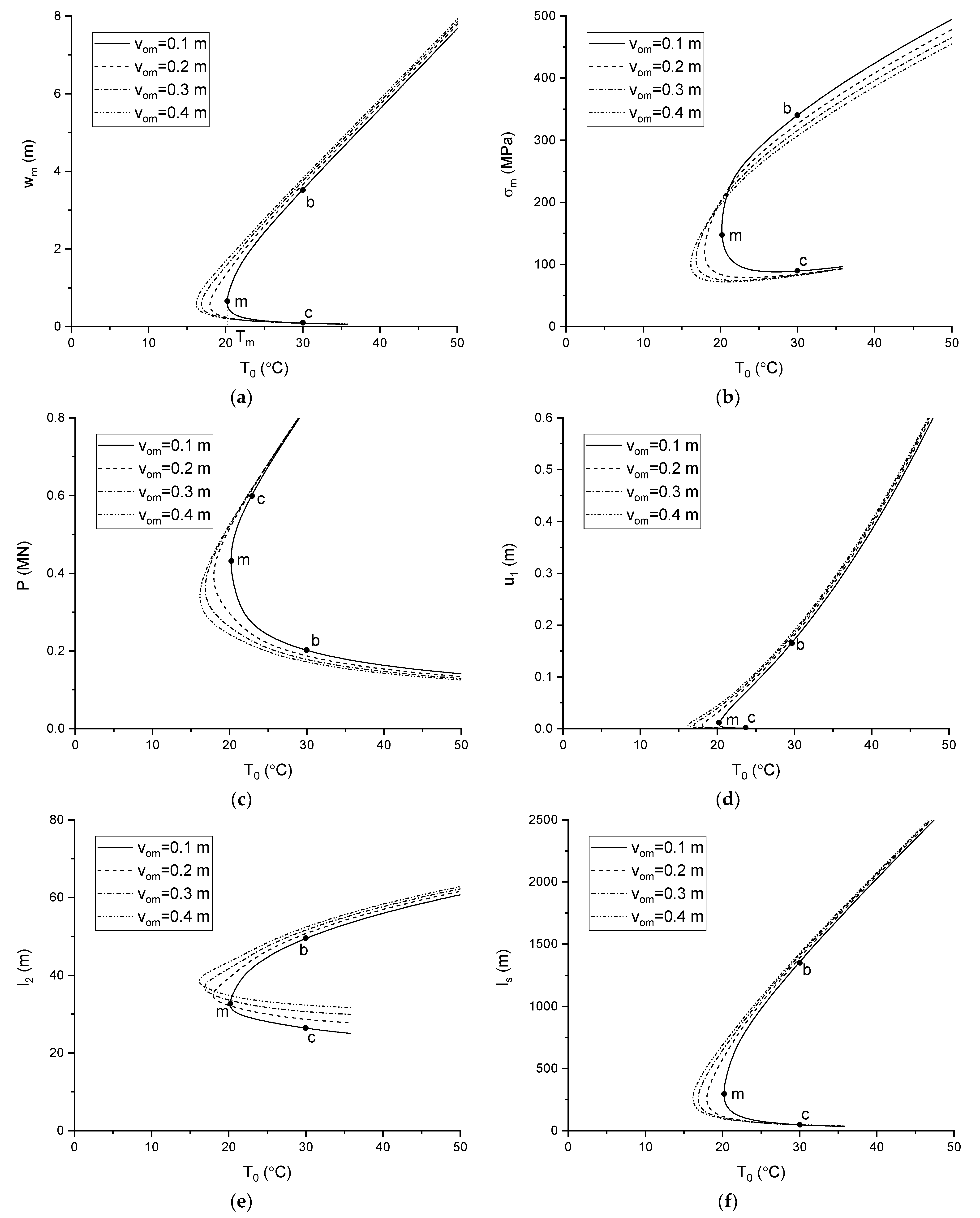
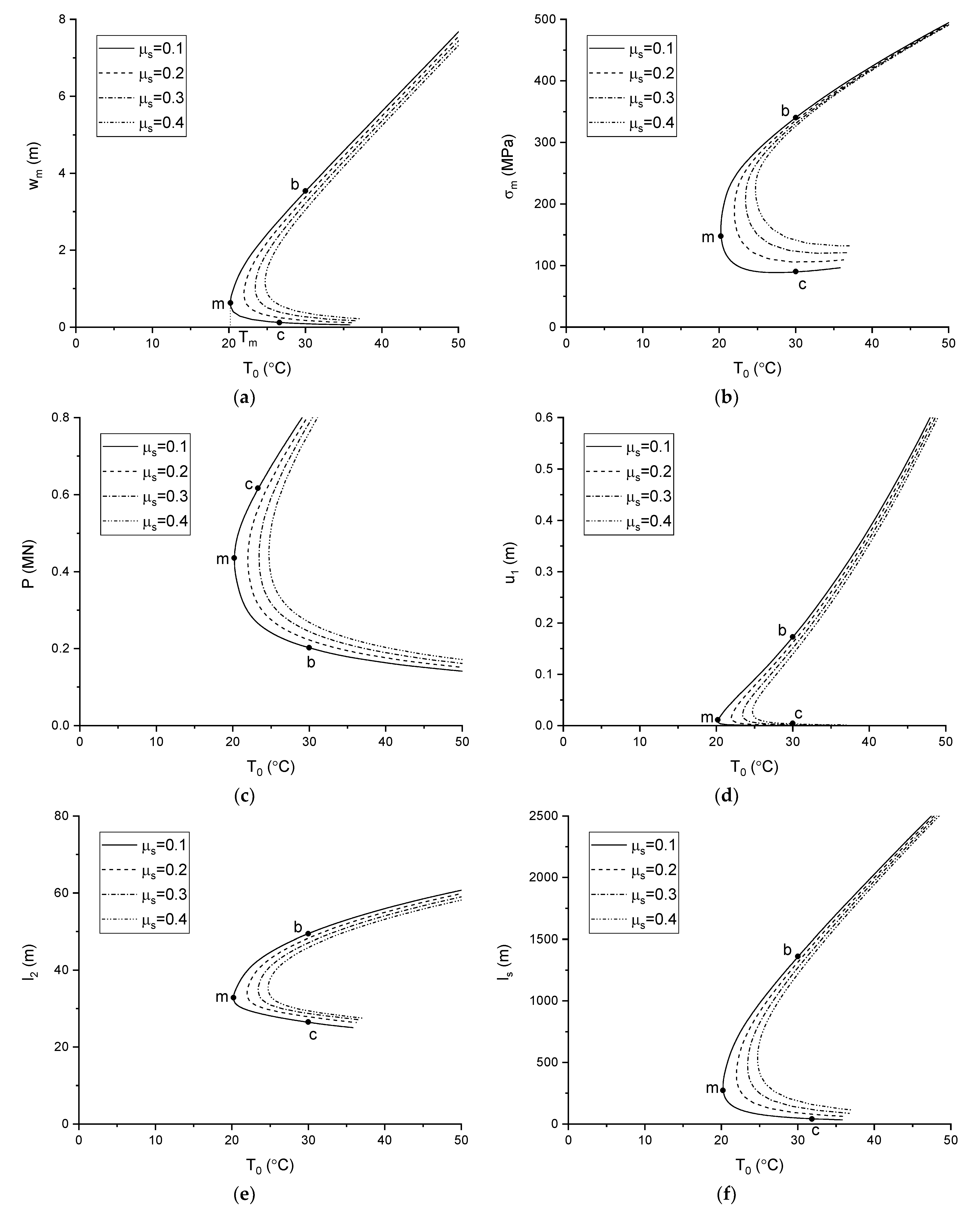
3.2.3. Influence of ${\mathsf{\mu }}_{\mathrm{s}}$

The influence of ${\mu }_s$ on the buckled configuration, post-buckling behaviour, and minimum critical temperature difference $T_m$ are shown in Figure 13, Figure 14 and Figure 15, respectively.

In Figure 13a, the deflection of the buckled pipeline shrinks with larger ${\mu }_s$. This is because the friction force between the pipeline and the sleeper becomes larger with larger ${\mu }_s$, which restricts the deflection of the buckled pipeline. In Figure 13b, the extrema of the bending stress in the positive direction becomes slightly larger with larger ${\mu }_s$. However, both the local minimum and the local maximum (absolute value) of the bending stress close to the sleeper in the negative direction become smaller with larger ${\mu }_s$, as shown in Figure 13b. With larger ${\mu }_s$, the difference between the local minimum and the local maximum of the bending stress close to the sleeper becomes larger. Taking ${\mu }_s=0.4$ as an example, it is clear that the local minimum (absolute value) of the bending stress is smaller than the local maximum (absolute value) of the bending stress.

In Figure 14a, $T_m$ is larger with larger ${\mu }_s$. The effect of ${\mu }_s$ on $T_m$ is illustrated in Figure 15, with different values of ${\mu }_{brk}$ and $v_{om}$. In Figure 15, $T_m$ increases with increasing ${\mu }_s$ for specific values of ${\mu }_{brk}$ and $v_{om}$, and the increasing rate of $T_m$ slightly reduces with increasing ${\mu }_s$. The friction force between the sleeper and the pipeline becomes larger with larger ${\mu }_s$, which makes it more difficult to trigger the lateral buckling. In Figure 15a, at the same ${\mu }_s$, $T_m$ becomes larger with larger ${\mu }_{brk}$. The increasing rate of $T_m$ with increasing ${\mu }_s$ is similar for different values of ${\mu }_{brk}$. In Figure 15b, under the same ${\mu }_s$, $T_m$ becomes smaller for larger $v_{om}$. The increasing rate of $T_m$ with increasing ${\mu }_s$ is larger for larger $v_{om}$. The influence of $v_{om}$ on $T_m$ gradually reduces with increasing ${\mu }_s$. Thus, the friction coefficient between the sleeper and the pipeline ${\mu }_s$ should be carefully controlled. When the value of ${\mu }_s$ is too large, such as ${\mu }_s=0.6$, $T_m$ is barely affected by the sleeper height $v_{om}$.

In Figure 14a,e, under a specific $T_0$, both $w_m$ and $l_2$ reduce with larger ${\mu }_s$. This is because, since the friction force between the sleeper and the pipeline becomes larger with larger ${\mu }_s$, the deflection of the buckled pipeline is restricted by the larger resistance between the sleeper and the pipeline. Thus, the requirements of both $u_1$ and $l_s$ decrease with larger ${\mu }_s$, as shown in Figure 14d,f. Due to the restriction of the larger friction force between the sleeper and the pipeline, the axial force $P$ increases with increasing ${\mu }_s$, as shown in Figure 14c. However, the maximum stress ${\sigma }_m$ along the buckled pipeline reduces with larger ${\mu }_s$ (see Figure 14b), which is induced by the decrease in the maximum bending stress (absolute value) along the buckled pipeline.

4. Conclusions

Through a consideration of the nonlinear pipe–soil interaction model, a mathematical model was proposed to simulate the lateral buckling of subsea pipelines triggered by a sleeper. The model was solved numerically and validated by comparing its predictions with the analytical solutions from [26]. The discrepancy between the numerical and analytical solutions was analysed through the discussion of the mobilization distance. A detailed parametric analysis was presented to show the effect of the breakout resistance, sleeper height, and sleeper friction coefficient on the buckling behaviour of a pipeline laid on a sleeper. The conclusions are:

(i)

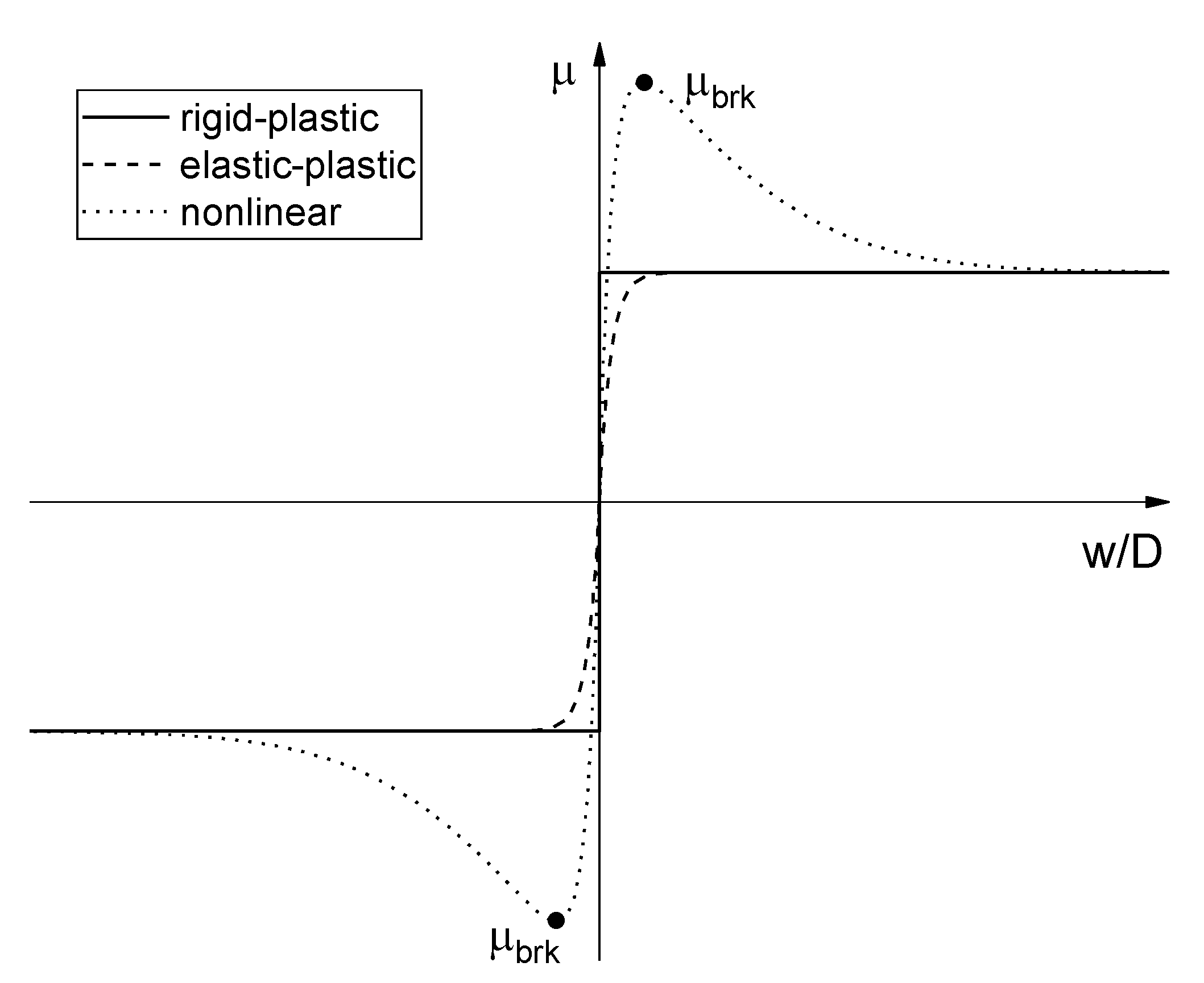
The discrepancy between the numerical and analytical solutions comes from the difference between the elastic-plastic and rigid-plastic pipe–soil interaction models, which reduces with decreasing mobilization difference in the elastic-plastic pipe–soil interaction model.

(ii)

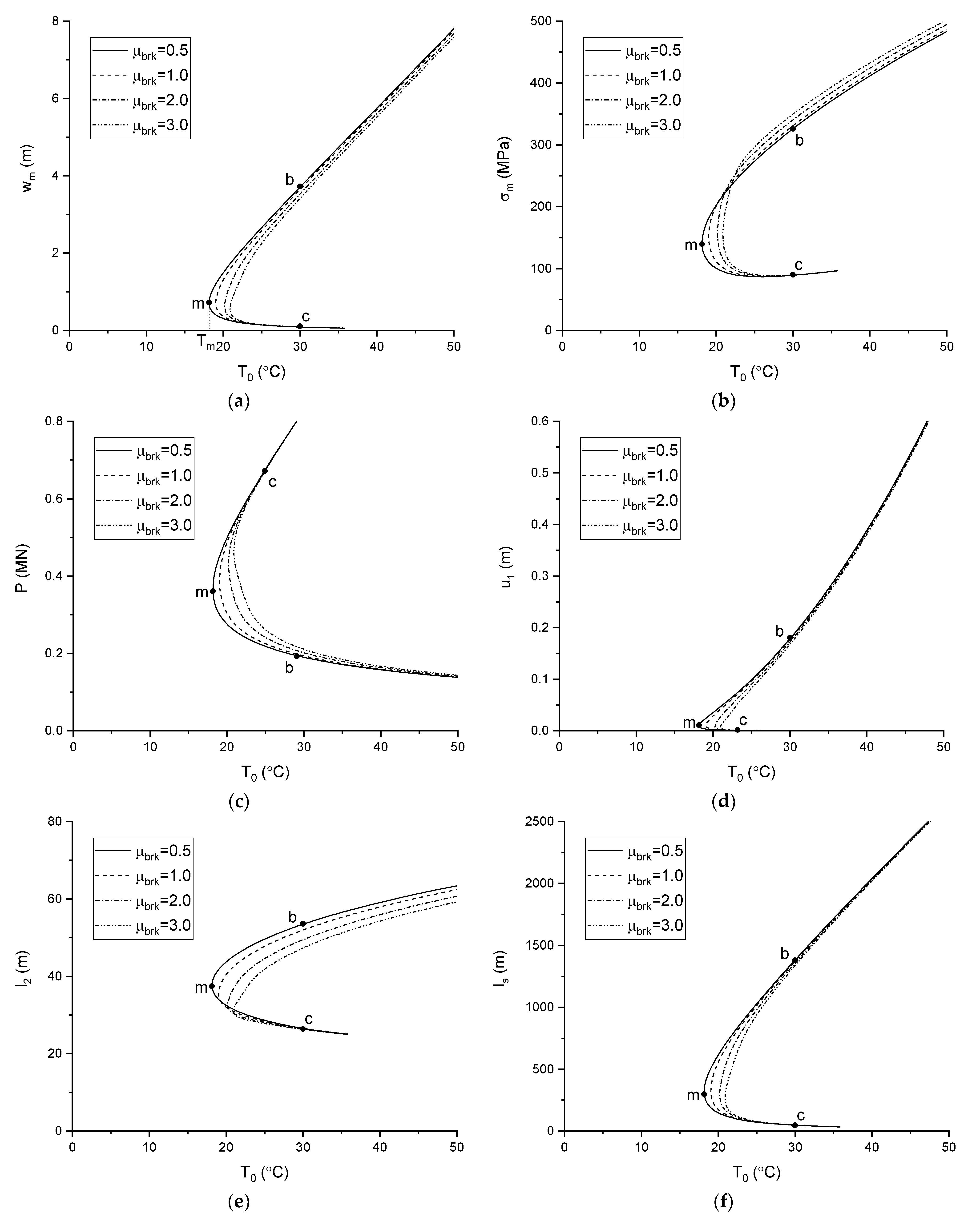
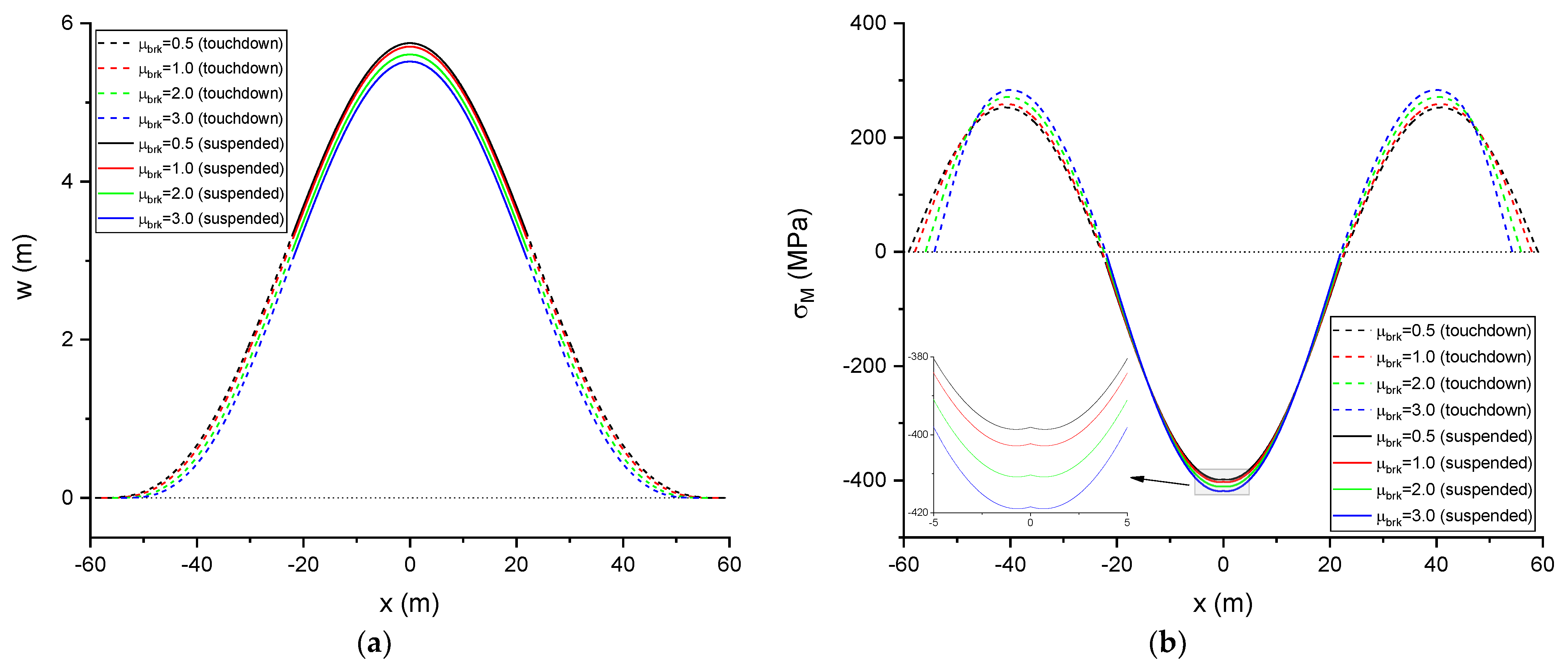
When the nonlinear pipe–soil interaction model is taken into account, both the displacement amplitude and the buckled length reduce due to the occurrence of breakout resistance, which decreases further with increasing breakout resistance. However, both the axial force and the maximum stress, along with the buckled pipeline, increase, and increase further with increasing breakout resistance.

(iii)

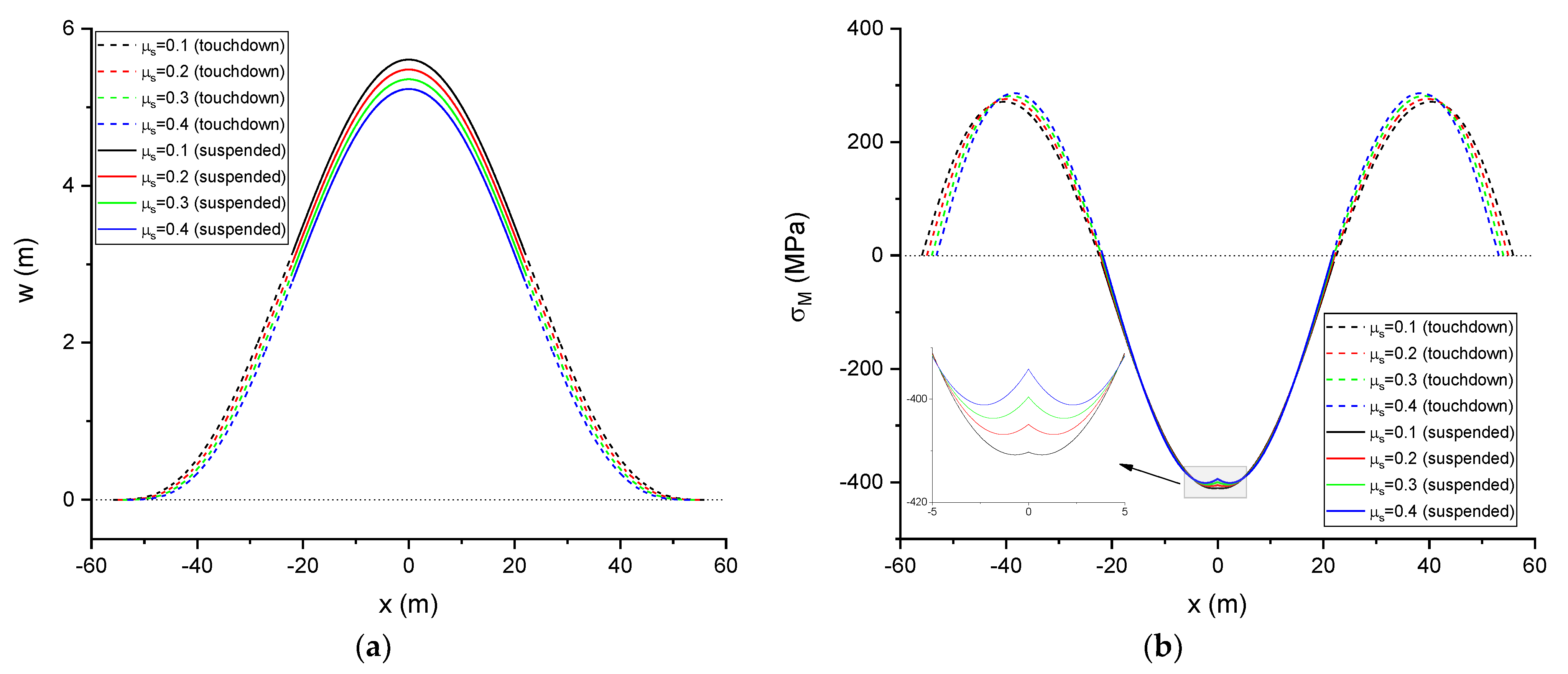
The deflection of the buckled pipeline enlarges as the sleeper height increases and shrinks as the sleeper friction coefficient increases. The axial force decreases with increasing sleeper height and increases with increasing sleeper friction coefficient. Moreover, the maximum stress along the buckled pipeline decreases with increasing sleeper height and with decreasing sleeper friction coefficient.

(iv)

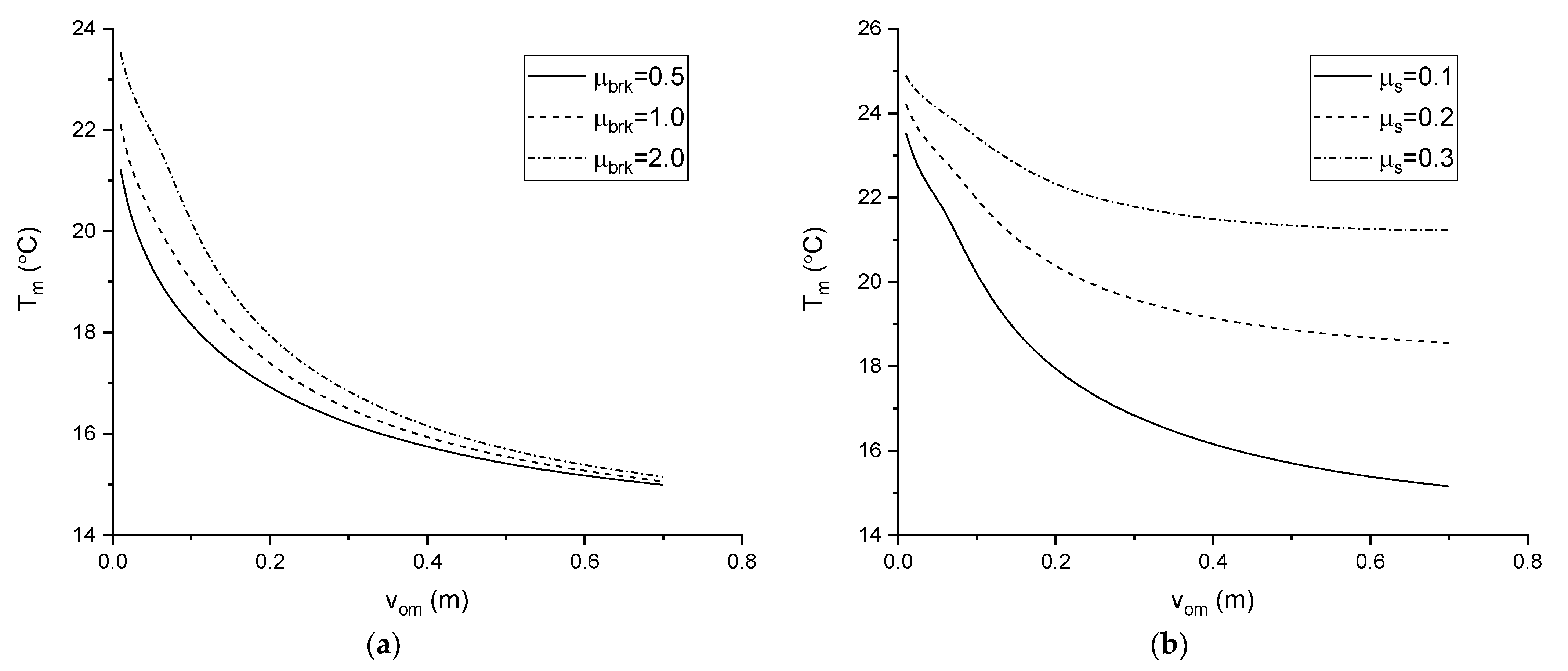
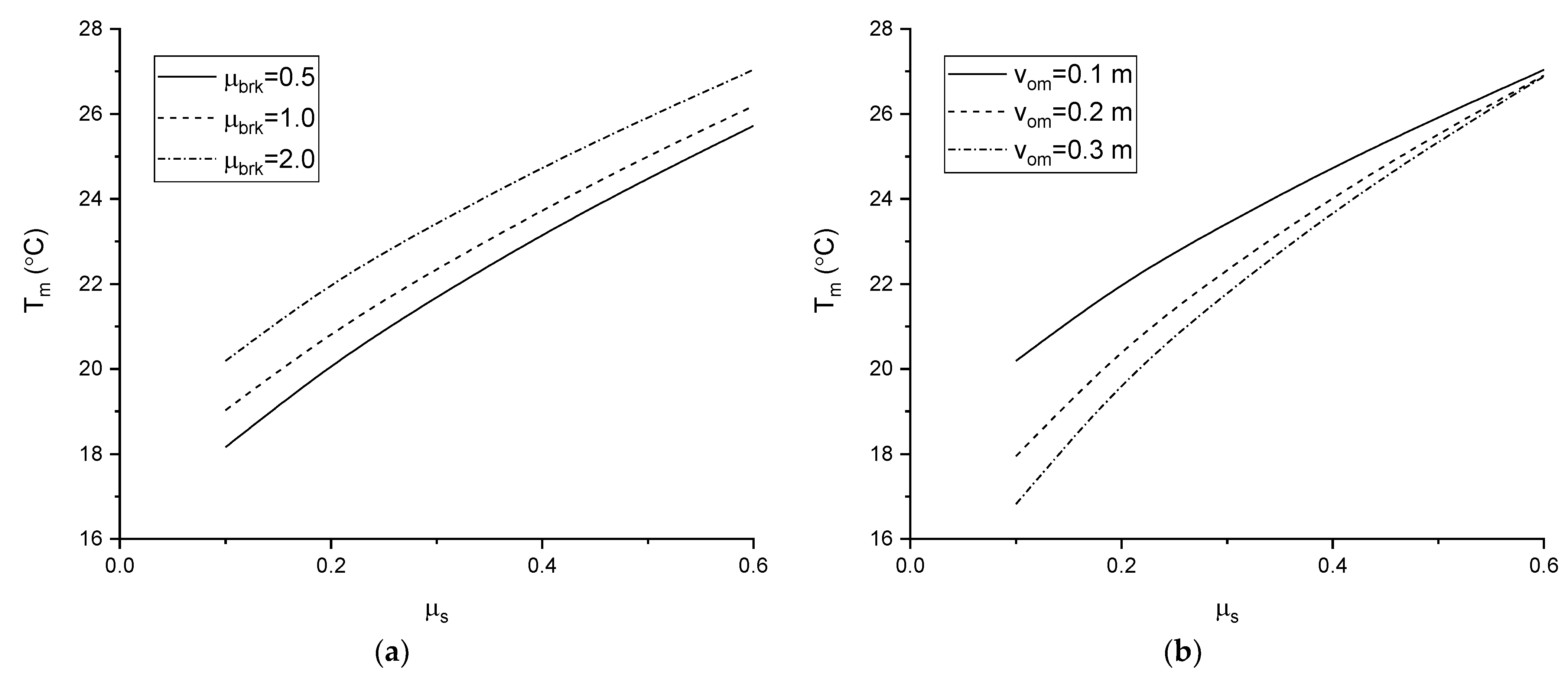
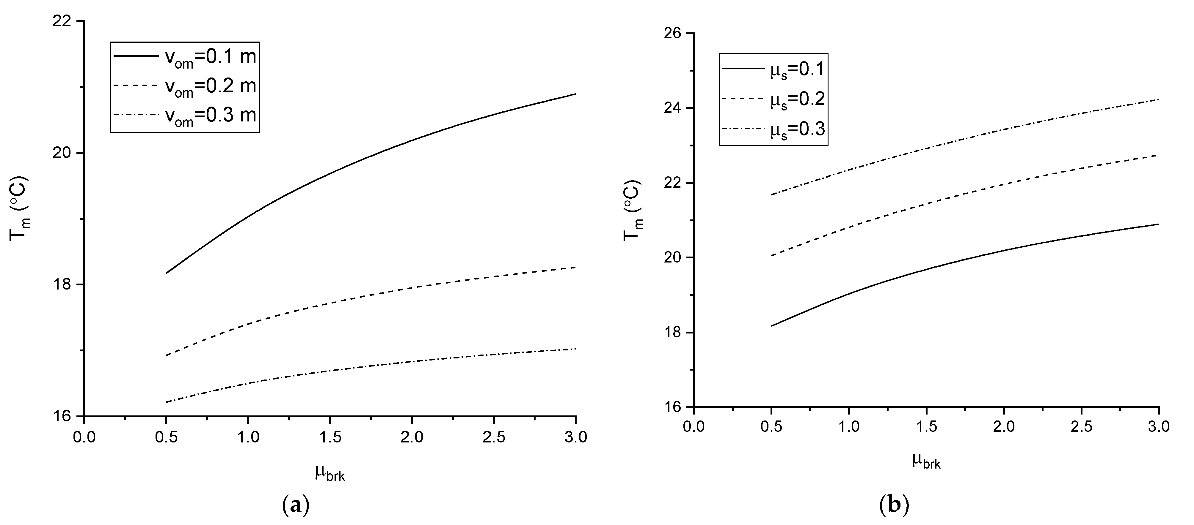
The minimum critical temperature difference increases with increasing breakout resistance and sleeper friction coefficient, and decreases with increasing sleeper height. The influence of the breakout resistance on the minimum critical temperature difference gradually reduces with increasing sleeper height. Moreover, the sleeper height has little effect on the minimum critical temperature difference when the sleeper friction coefficient is large enough.

In conclusion, it is better to incorporate the nonlinear pipe–soil interaction model into the mathematical model when simulating the lateral buckling of subsea pipelines triggered by a sleeper, since both the minimum critical temperature difference and the maximum stress increase. Moreover, both the sleeper height and the sleeper friction coefficient should be carefully selected and controlled.

References

- DNV-RP-F110; Global Buckling of Submarine Pipelines. Det Norske Veritas: Oslo, Norway, 2019.
- Hobbs, R.E. In-service buckling of heated pipelines. J. Transp. Eng. 1984, 110, 175–189. [Google Scholar] [CrossRef]
- Taylor, N.; Gan, A.B. Submarine pipeline buckling-imperfection studies. Thin-Walled Struct. 1986, 4, 295–323. [Google Scholar] [CrossRef]
- Croll, J.G.A. A simplified model of upheaval thermal buckling of subsea pipelines. Thin-Walled Struct. 1997, 29, 59–78. [Google Scholar] [CrossRef]
- Karampour, H.; Albermani, F.; Veidt, M. Buckle interaction in deep subsea pipelines. Thin-Walled Struct. 2013, 72, 113–120. [Google Scholar] [CrossRef] [Green Version]
- Liu, R.; Xiong, H.; Wu, X.; Yan, S. Numerical studies on global buckling of subsea pipelines. Ocean Eng. 2014, 78, 62–72. [Google Scholar] [CrossRef]
- Hong, Z.; Liu, R.; Liu, W.; Yan, S. Study on lateral buckling characteristics of a submarine pipeline with a single arch symmetric initial imperfection. Ocean Eng. 2015, 108, 21–32. [Google Scholar] [CrossRef]
- Liu, R.; Wang, X. Lateral global buckling high-order mode analysis of a submarine pipeline with imperfection. Appl. Ocean. Res. 2018, 73, 107–126. [Google Scholar] [CrossRef]
- Konuk, I. Coupled lateral and axial soil-pipe interaction and lateral buckling Part II: Solutions. Int. J. Solids Struct. 2018, 132–133, 127–152. [Google Scholar] [CrossRef]
- Konuk, I. Coupled lateral and axial soil-pipe interaction and lateral buckling Part I: Formulation. Int. J. Solids Struct. 2018, 132–133, 114–126. [Google Scholar] [CrossRef]
- Zhang, X.; Duan, M. Prediction of the upheaval buckling critical force for imperfect submarine pipelines. Ocean Eng. 2015, 109, 330–343. [Google Scholar] [CrossRef]
- Zhang, X.; Guedes Soares, C.; An, C.; Duan, M. An unified formula for the critical force of lateral buckling of imperfect submarine pipelines. Ocean Eng. 2018, 166, 324–335. [Google Scholar] [CrossRef]
- Liu, R.; Li, C. Determinate dimension of numerical simulation model in submarine pipeline global buckling analysis. Ocean Eng. 2018, 152, 26–35. [Google Scholar] [CrossRef]
- Zeng, X.; Duan, M. Mode localization in lateral buckling of partially embedded submarine pipelines. Int. J. Solids Struct. 2014, 51, 1991–1999. [Google Scholar] [CrossRef] [Green Version]
- Chee, J.; Walker, A.; White, D. Effects of variability in lateral pipe-soil interaction and pipe initial out-of-straightness on controlled lateral buckling of pre-deformed pipeline. Ocean Eng. 2019, 182, 283–304. [Google Scholar] [CrossRef]
- Zhang, X.; Guedes Soares, C. Lateral buckling analysis of subsea pipelines on nonlinear foundation. Ocean Eng. 2019, 186, 106085. [Google Scholar] [CrossRef]
- Peek, R.; Yun, H. Flotation to trigger lateral buckles in pipelines on a flat seabed. J. Eng. Mech. 2007, 4, 442–451. [Google Scholar] [CrossRef]
- Shi, R.; Wang, L. Single buoyancy load to trigger lateral buckles in pipelines on a soft seabed. J. Eng. Mech. 2015, 141, 1–7. [Google Scholar] [CrossRef]
- Wang, Z.; Tang, Y. Antisymmetric thermal buckling triggered by dual distributed buoyancy sections. Mar. Struct. 2020, 74, 102811. [Google Scholar] [CrossRef]
- Chee, J.; Walker, A.; White, D. Controlling lateral buckling of subsea pipeline with sinusoidal shape pre-deformation. Ocean Eng. 2018, 151, 170–190. [Google Scholar] [CrossRef] [Green Version]
- Silva-Junior, H.C.; Cardoso, C.O.; Carmignotto, M.A.P.; Zanutto, J.C. Reduced Model Device of Solutions to Control Thermal Buckling Effects in HP-HT Subsea Pipelines (OMAE2008-57637). In Proceedings of the International Conference on Ocean, Offshore and Arctic Engineering, Estoril, Portugal, 15 June 2008. [Google Scholar]
- de Oliveira Cardoso, C.; Solano, R.F. Performed of triggers to control thermal buckling of subsea pipelines using reduced scale model (ISOPE-I-15-445). In Proceedings of the International Offshore and Polar Engineering Conference, Honolulu, HI, USA, 21–26 June 2015. [Google Scholar]
- Bai, Q.; Qi, X.; Brunner, M. Global buckle control with dual sleepers in HP/HT pipelines (OTC-19888-MS). In Proceedings of the Offshore Technology Conference, Houston, TX, USA, 4–7 May 2009. [Google Scholar]
- Wang, Z.; Tang, Y. Analytical study on controlled lateral thermal buckling of antisymmetric mode for subsea pipelines triggered by sleepers. Mar. Struct. 2020, 71, 102728. [Google Scholar] [CrossRef]
- Hong, Z.; Liu, W. Modelling the vertical lifting deformation for a deep-water pipeline laid on a sleeper. Ocean Eng. 2020, 199, 107042. [Google Scholar] [CrossRef]
- Wang, Z.; Tang, Y.; van der Heijden, G.H.M. Analytical study of lateral thermal buckling for subsea pipelines with sleeper. Thin-Walled Struct. 2018, 122, 17–29. [Google Scholar] [CrossRef] [Green Version]
- Lagrange, R.; Averbuch, D. Solution methods for the growth of a repeating imperfection in the line of a strut on a nonlinear foundation. Int. J. Mech. Sci. 2012, 63, 48–58. [Google Scholar] [CrossRef]
- Wang, Z.; Tang, Y.; van der Heijden, G.H.M. Analytical study of distributed buoyancy sections to control lateral thermal buckling of subsea pipelines. Mar. Struct. 2018, 58, 199–222. [Google Scholar] [CrossRef] [Green Version]
- Chatterjee, S.; White, D.J.; Randolph, M.F. Numerical simulations of pipe-soil interaction during large lateral movements on clay. Géotechnique 2012, 62, 693–705. [Google Scholar] [CrossRef]
- Wolfram Mathematica, version 11.0; Wolfram Research, Inc.: Champaign, IL, USA, 2016.