Abstract
In this paper, the state-of-the-art concerning new methodologies for surveying in coastal areas in order to obtain an efficient quantification of submerged and emerged environments is described and evaluated. This work integrates an interdisciplinary approach involving both geomatics and robotics and focuses on definition, implementation, and development of a methodology to execute integrated aerial and underwater survey campaigns in shallow water areas. A preliminary test was performed at Gorzente Lakes near Genoa (Italy), to develop and integrate different survey techniques, enabling working in a smarter way, reducing costs and increasing safety for the operators. In this context, Remote Sensing techniques were integrated with a UAV (Unmanned Aerial Vehicle) carrying an aerial optical sensor for photogrammetry and with an ASV (Autonomous Surface Vehicle) expressly addressed to work in extremely shallow water with underwater acoustic sensors (single echo sounder). The obtained continuous seamless DSM (Digital Surface Model) for the entire environment was reconstructed by the combination of different sensing systems by limiting reliance on the GNSS (Global Navigation Satellite System) support. The obtained DSM was displayed in a 3D model leading to the evaluation of the water flow volume and rendering of 3D visualization.
1. Introduction
Topographic and bathymetric surveys have been widely applied to investigate and monitor the evolution of the occurred geomorphological processes [1,2]. A wide range of techniques to measure topography and bathymetry exist to obtain the measurement requirements, in terms of precision, accuracy, cost effectiveness and in reasonable time. Despite the multiple available methods and techniques, the collected data from emerged and submerged environments rely on distinct equipment and techniques at different times and are obtained with assorted accuracy and spatial resolution [3,4,5,6]. Subsequently, several methods have been proposed to combine two datasets in order to achieve a holistic knowledge of these environments [7,8,9,10,11]. The goal is to achieve a continuous model as an output between the two environments [6]. Existing approaches, ranging from traditional techniques (e.g., bathymetric vessels, total stations and GNSS to the latest innovations, thanks to the rapid technological evolution of remote sensing (e.g., photogrammetry, laser scanner, LiDAR (light detection and ranging) and acoustics senors), support the opportunity to obtain a huge amount of data [8,9,10]. The availability of several sensors and techniques leads to various methods of combing datasets, which are determined in correspondence with the used sensors [6]. Generally, acquiring data from different environments (i.e., bathymetric and topographic data) leads to better quality by using a dedicated sensor for each environment. This is due to the different specifications for each sensor that influence the spatial resolution of measurements. In light of this, investment of the available resources and the collected data from distinct sensors and working on building a methodology to combine the diverse nature of datasets [12] create the prospect of generating a precise seamless DSM (Digital Surface Model) between emerged and submerged environments [11,13]. To apply a separate methodology for survey execution in a shallow water area, nowadays bathymetric measurements are performed with acoustic methods, mostly by relying on a single beam echosounder and a multi beam echosounder that have recently been considered the basis of most hydrographic surveys [6,14]. This is due to the capability of providing the most accurate results. On the other hand, the photogrammetric survey is becoming one of the most cost-effective techniques for topographic surveys in terms of time and effort [15] as well as in terms of accuracy and coverage. The common nature of the product from these different sensors is presented as a point cloud that eases the merging process of the two datasets. Additionally, MLS (Mobile Laser Scanner) can be mounted on USV (Unmanned Surface Vessel), which is considered an efficient solution to providing data overlapping both environments (emerged and submerged zones) [14,15]. This technique can support combing topographic and bathymetric datasets in shallow water areas, since it ensures the continuity of data in the littoral zone. From a different perspective, a different conceptual methodology to acquire a combined model between the emerged and submerged zones is using a common technique. LiDAR is considered as a solution technique used to provide a combined continuous model between emerged and submerged areas [6,14,15]. The fact that topographic and bathymetric LiDAR sensors have a different specification, which leads to a different accuracy, vertical datum, resolution and data elaboration [6,13]. Among photogrammetric techniques, there is a substantial new photogrammetric technique called Structure from Motion (SfM), which permits the generation of a 3D model in coastal areas as emerged and submerged zones through algorithms including camera motion [6,16]. Hence, unlike conventional photogrammetry, SfM needs highly calibrated cameras and stable imaging geometry through advanced computation. Similar to the photogrammetric approach, SfM relies on the overlapping between consecutive images to have the ability to reconstruct a 3D model starting from 2D images [16]. The output product of this technique as a point cloud has a spatial resolution that is generally comparable to LiDAR, highlighting that the achieved accuracy of the bathymetric measurements are related to several environmental issues such as seafloor texture, water clarity and effective depth [6]. The difficulties in creating a single coherent DSM for emerged and submerged zones are related to the vertical datum variation between bathymetric and topographic measurements, e.g., bathymetric measurements are related to the variation occurring in the water level. Moreover, the occurrence of horizontal gaps due to merging two datasets impacts the reliability and continuity of the obtained DSM [13]. The use of SWAMP ASV, capable of working and collecting SBES data in less than 15 cm of water, allows us to obtain data at the boundary layer between land and water, thus providing the possibility of integrating the data in a better way. This increases the reliability of the proposed method. The survey campaign was carried out, limiting the use of the GNSS support, since this technique could be susceptible to some limitations due to the lacking satellite visibility or the eventual presence of electromagnetic interference, e.g., in harbor environments. Hence, efficient survey planning and realization, together with well processing capability, allow us to attain high quality results [7]. Furthermore, the contribution of obtaining a continuous and seamless DSM consists of generating a 3D model that is useful for modeling water flow and rendering of 3D visualizations and analysis for the study area. The paper is organized as follows: Materials and Methods are addressed and illustrated in broad context together with the description of the targeted study area in Section 2; the obtained results and their discussion are presented in Section 3 and Section 4, respectively. The paper closes by providing the conclusions, in accordance with the highlighted results and discussion.
2. Materials and Methods
This section is dedicated to the detailed description of the techniques (Section 2.1) employed to survey the study area (Section 2.2), exploiting the proposed integrated method (Section 2.3).
2.1. Materials
From the authors’ field experience [15], the primary obstacle to working on different environments using distinct instruments consists of the occurrence of gaps between the resulting datasets [13]. Mostly, the scarcity of acquiring hydrographic data from shallow water (below 1 m) is inextricably linked to the lack of hydrographic vessels capable of carrying out measurements in similar environments [17]. However, in the present work, the interdisciplinary approach was the key to overcoming this difficulty. In this context, robotics as SWAMP (Shallow Water Autonomous Multipurpose Platform) [17] provide the contribution to acquiring data through land/water interface zones. SWAMP is an ASV (Autonomous Surface Vehicle) the characteristics of which can be modified and correlated to the mission specifications. It is a catamaran 1.23 m long and 1.1 m wide. The hull height is 0.4 m; including the structure and communication antennas; it is 1.1 m high. SWAMP is considered a small and lightweight (38 kg) vehicle adequate to be transportable by hand; this is particularly useful in areas where access is limited. SWAMP’s flexible design is adequate for hosting different tools, e.g., thrusters, control systems, samplers and sensors. SWAMP is based on the use of four pump-jet thrusters [18] the configuration of which allows for the efficient control that is especially required in shallow water zones for high quality survey and performance [19]. The bathymetric survey measurements were performed by using an ultra-compact precision SBES (Single Beam Echo Sounder) Echologger ECS400 with 200 kHz frequency mounted inside the SWAMP hull. The vertical measurements were performed by the SBES with an altimetric resolution better than 1 mm, with real time backscatter data collection along the water column up to a depth rate equivalent to 1000 m. SBES measurements were synchronized with an IMU (Inertial Measurement Unit) sensor provided by a Microstrain 3DM-GX3-35, a high-performance, miniature AHRS (Attitude Heading Reference System) with GPS (Global Positioning System) that was present on board and provided absolute orientation (yaw, pitch and roll), and with a Drotek DP0106 absolute position sensor that provided GNSS positions during data collection. The SBES sensor performs bathymetric measurements directly beneath the sensor itself, providing only depth information along the track line of the vehicle. The SBES depth measurements were based on measuring the acoustic pulse travel time from the transducer to the waterway bottom and back to the receiver. Hence, auxiliary information about sound speed in water is essential. Generally, sound velocity ranges between 1400 and 1600 m/s; depending on water characteristics, when a sound velocity profile is not available through the water column, the echosounder system uses average sound velocity as 1500 m/s [12,20]. SBES is the most common survey technique used in lake and river environments, because of its efficiency, low cost and accessibility [3,12,19]. Considering the SBES resolution, the acquired data are considered precise and cost effective. Instead, for big data coverage, it is more efficient to use MBES to have more precise DSM generation with the highlight that this system is more expensive. According the IHO standards [21], the survey could be considered 1b, since the survey was performed in a lake environment, so not related to safety of navigation. When using SBES, inspection converge rate is limited. Higher standards could be achieved by using MBES, which provides more coverage. Like bathymetric data collection, topographic data collection relies on robotic vehicles. UAV photogrammetry was performed through a 20 MPx camera mounted on a DJI Mavic 2 Pro. The proper overlapping between images was obtained by extracting them from a video with a frame rate of one image per second, leading to a percentage of 70% overlapping for both forward and side directions. Further images were taken with terrestrial close-range photogrammetry by the embedded camera of a smartphone with a 24.8 MPx sensor size. The resulting 649 images, coming from both UAV and terrestrial photogrammetry, were processed by means of the photogrammetric software Agisoft Metashape© (V 1.8.2) [22], producing a 3D point cloud by merging four different image datasets based on the single shooting geometries, i.e., nadiral or facing the object. Each image dataset covers a portion of the study area, such that they are mutually complementary. To compute the distributed Ground Control Points (GCPs) coordinates, Total Station Leica TC703 was used with a display resolution equivalent to 1 mm. The employed instruments are shown in (Figure 1).
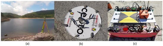
Figure 1.
Instrumentation used through the survey campaign execution; (a) the Total station, (b) the UAV to perform topographic photogrammetric survey, (c) the SWAMP that carried out the bathymetric survey.
2.2. Study Area
The study was carried out on a small portion (20,550 m2) of Laghi del Gorzente, located in the provinces of Genoa (Liguria) and Alessandria (Piedmont). Laghi del Gorzente are three artificial basins produced by the dams and they serve as a retention structure and water storage for ecosystem conservation by reviving the environment which is itself rather barren. The study area has a funnel-shape that lies embedded in a steep valley. The land cover surrounding the lake with a steep bare slope is characterized by mixed sedimentation, composed of a combination of rocky coast, gravels, sand and silt with tall trees on the outer boundaries which sets a natural limit to the lake. The study area is shown in (Figure 2).
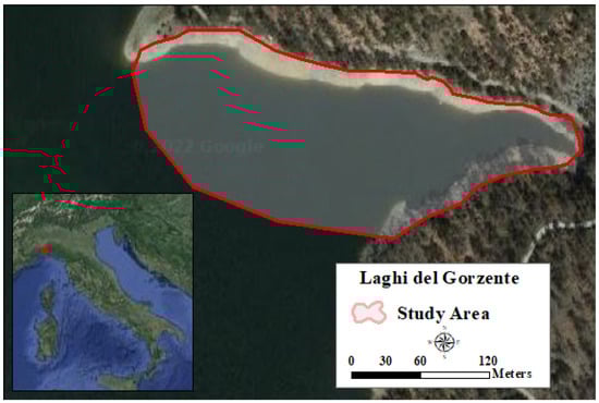
Figure 2.
Study area targeted (emerged and submerged zones) over Laghi del Gorzente.
The water level depends on the water flows to the lake; periods of null-discharge flows are frequent, mostly during summer, as well as floods in winter or spring. Since no database in terms of bathymetric measurements and accurate merging with topographic surface is available, integrated survey measurements have been carried out in this area to analyze the bathymetry of this watercourse. Moreover, obtaining three-dimensional information corresponding to this area is a significant contribution to extending the existing national databases. Furthermore, as the coastal areas survey is affected by the water surface and wave action, then the survey performance in a steady environment such as a lake represents the ideal conditions in which to examine and evaluate new survey methodologies. These factors, aside from the legal/social constraints, in terms of the possibility to execute a survey campaign in the targeted area, made it a convenient location to examine the efficiency of the proposed measurement methodology.
2.3. Methods
In this section, the survey techniques and methods carried out in the study area are presented. The interdisciplinary and integrated approach through integrating several survey techniques, i.e., photogrammetry from the UAV and smartphone, the SBES mounted on SWAMP, and the Total station, is described in the following (Figure 3).
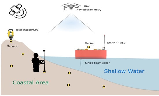
Figure 3.
Interdisciplinary approach by using several techniques to perform integrated survey campaign over different environments (emerged and submerged zones).
The rapid technological evolution of robotics and sensing techniques imposes an alternative surveying approach rather than conventional techniques. The authors believe that selecting suitable survey techniques and methods is pertinent. At present, the main task is to achieve precise data merging acquired from submerged and emerged environments, considering cost effectiveness and timing. Consequently, SBES was nominated as an efficient and cost-effective technology to perform a bathymetric survey in steady environments such as lakes [3,12,19]. However, if the goal is to achieve a reliable combination of data from both environments, SWAMP was presented as a surface vehicle capable of acquiring bathymetric information in an area of less than 1 m depth [17]. Despite the cost-efficiency benefits, SWAMP will provide a solution to improve the capability to acquire data from less accessible areas and to extend new standards in terms of accuracy. Obviously, auxiliary information is necessary [8,12] to obtain and georeference the collected measurements. These are provided by the on-board IMU sensor providing absolute orientation (yaw, pitch and roll) and the GNSS sensor providing an absolute position. One essential aspect is correlated to attain a precise synchronization between all sensors performing measurements mounted on the SWAMP, as well as to obtain a common reference frame joining all measurements executed through the survey. Moreover, the sound velocity profile through water column must be considered for bathymetric measurements. In this case, due to the absence of the sound velocity profile, a standard sound speed such as 1500 m/s in water is considered. The acquisition is automatic, and the outputs are metrically reliable and provided in a short time [8]. On the other hand, expert operators are required to setup and calibrate the system and to acquire and process the data. Moving forward to the photogrammetric technique, the effectiveness of the mentioned technology is represented mainly in the huge coverage of data provided and the semi-automatic processing of data that acquire a less experienced operator [15]. Additionally, a great advantage is related to the low cost of the instrumentation. Mostly, the photogrammetric survey is carried out by an optical sensor mounted on a UAV and images are taken from the nadir view of the area of interest. Obviously, by applying photogrammetry and obtaining sufficient overlapping between consecutive images, then it is possible to reconstruct a digital 3D model of the surveyed environment by processing the data [7,8,23]. However, optimized survey planning and locating a sufficient number of well distributed Ground Control Points (GCPs), coupled with processing capabilities, were needed to build an accurate metric 3D model in terms of adequate accuracy and precision. The performed flight was constrained by interference issues that obliged the pilot to stay at 30 m AGL. In order to obtain a full coverage for the surveyed area, a video along two strips was collected at the allowed distance of 30 m. This resulted in high-resolution images with 7 mm of GSD. The study area was divided into four portions, surveying them separately with different shooting geometries and techniques. In fact, two portions were surveyed by relying on the mentioned recording videos from the UAV, while for the rest, images were collected from the smartphone in lateral view, with attention to be paid to the overlapping between images. However, obtaining images with several techniques and orientations implies more processing efforts to achieve a final photogrammetric 3D model comparable with the expected accuracy [8,20,24]. Aside from what is stated, the correlation between the well GCPs’ distribution over the study area and the obtained accuracy is comprehensible to the authors. Hence, considering the study area’s morphology and dimension, 19 markers were distributed with 20 m separation between two consecutive markers according to a net-like shape, depending on the need to pick a sufficient number of markers in common among the collected images. GCPs were measured by means of the total station, mainly because the methodology relies on limiting the use of GNSS to have the possibility to apply to harbor environments where the use of GNSS may be problematic due to the high electromagnetic interference, and due to the fact of the presence of electromagnetic radiations that cut off the GNSS signal. On this occasion, the total station was an alternative opportunity to determine the positions and heights of points, instead of GNSS, with consequently more effort needed to place and survey the GCP, especially in inaccessible areas such as locations where steep slope areas exist [3]. Moreover, the choice of the location of the total station in the field was properly managed taking into account the visibility between the total station and the prism put on all the GCPs markers in the field. Image alignment was performed on a medium accuracy relying on the GCPs measurements for the four subsets of images using Agisoft Metashape© software. The choice of the accuracy rate in the image alignment process must tie in with the expected accuracy and the duration of data processing, e.g., the highest accuracy setting is recommended only for very sharp image data and corresponding processing being quite time consuming. It has been noticed that stereo matching is challenging with images with low contrast levels such as sandy areas due to the high light exposure. On the basis of aligned images, a dense point cloud for the targeted area is generated. Generally, a dense point cloud is created by the software based on the exterior and interior image orientation parameters by calculating the depth maps for overlapping images estimated by bundle adjustment. Hence, the software generates a depth map for each camera position and combines them to create a merged dense point cloud. A dense cloud was built at a medium quality for each image dataset, knowing that the quality specifies the depth map generation of the obtained point cloud. Subsequently, several dense point clouds were merged into a single one representing the basis of GCPs coordinates. The digital images were orthorectified and combined into a mosaic with 2 cm/pixel resolution, for ground display. However, following the main objective, i.e., developing a method to integrate bathymetric and topographic data for creating a seamless and continuous DSM between the two environments, photogrammetry is not the best solution to identify the interface boundary between emerged and submerged zones, since, in that area, the achieved point clouds may not be reliable in terms of accuracy, due to the lack of GCPs in such areas coupled with the existence of refraction and reflection phenomena in the zones along the border. Therefore, the following question is raised: how do we integrate bathymetric data with topographic data obtained by different instrumentation and techniques [8,13]? Several aspects were considered before the survey execution. To identify the key issues that obstruct data integration, the authors addressed and highlighted these aspects: (1) differences between the vertical datum of topographic and underwater data [13]; (2) the occurrence of expected gaps between the two datasets will complicate the merging of data; (3) differences between the planimetric datum and the complexity due to the no-collocation of the sensors on the SWAMP. Indeed, in bathymetric measurements, heights or depths are initially related to sensor position [13]. This is done by measuring the distance between the sensor and the underwater ground. After that, the measurements will be transformed to the water level as a reference surface. On the contrary, the approach to establish vertical datum for topographic measurements is quite different because topographic measurements could be related to the geoid model or to the ellipsoidal reference, as with the ones derived from GNSS. However, conceptually, these two approaches should be producing comparable results. Hence, datum differences must be taken into account and treated during the survey data integration processes. The altimetric one uses the water level as a reference surface. For the planimetric datum shift, SWAMP was removed from the water after performing bathymetric measurements and was located on the ground in two different positions called Point 1 and Point 2, shown as red dots in (Figure 4).
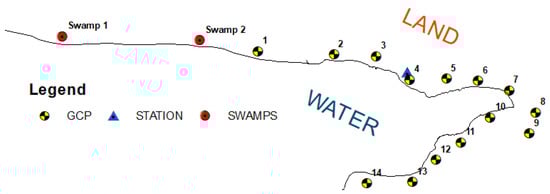
Figure 4.
Total station location (blue triangle), GCPs (black and yellow dots) distribution and the two locations of SWAMP on Point 1 and Point 2 (red dots).
A marker was attached to the SWAMP hull and measurements were performed by using the total station and prism to compute the local coordinates of the two different locations of SWAMP on the ground, i.e., Point 1 and Point 2. In parallel, the GPS mounted on SWAMP was recording measurements for the same two locations (Point 1 and Point 2). In this context, Point 1 and Point 2 are measured in two different reference systems, one related to the topographic reference system (local system) by total station, while the other related to the bathymetric reference system (WGS 84) by the GPS receiver mounted on SWAMP. A second step was represented by the transformation of the local coordinates points (measured by total station) to the WGS84, depending on the common control points—Point 1 and Point 2—in both systems. To perform this, the Autocad Civil 3D [25] software was employed. A common reference frame must be computed, because the GPS and the marker mounted on the SWAMP have different positions, so measurements from the total station and from GPS have been adequately attributed by referring them to the same point represented by the location of the marker. Furthermore, to obtain a common vertical reference frame between both environments, all measurements were referred to the real water surface level. Through the survey campaign, several points were measured by the total station to detect the position of the shoreline. The position of the shoreline, representing the strip where the water meets the land, was considered the reference vertical surface and as the zero level surface. In this context, all the measurements carried out have to be shifted with respect to the water surface level (zero level). It is necessary to note that, in order to integrate the two datasets, a better distribution of the locations of SWAMP on several topographic points (red points in Figure 4) permits a better evaluation of the planimetric roto-translation transformation. Unfortunately, different technical problems occurred during the survey and it was not possible to survey other markers with SWAMP (for example the markers number 7 and number 14) to connect the topographic and bathymetric datum, with a redundancy and well distributed set of common points. Hence, the approach was to deal with gaps to maintain the quality and continuity of the generated DSM [8,13]. The lower is the extension of gaps, the higher is the probability of obtaining a realistic, smooth and seamless integrated solution. In this context, aside from merging data in correspondence to the measured control points and zero level points measured on the shoreline, the contribution of digitizing the shoreline extracted from the georeferenced orthophoto carried out through the GIS (Geographic Information System) environment [26] was useful for obtaining a more reliable integration of the two datasets. Subsequently, Natural Neighbor Interpolation was carried out after merging both data to obtain a continuous DSM for the entire study area.
3. Results
This section is dedicated to presenting the final outputs by providing the calculated coordinates (Section 3.1), displaying the resulting topographic (Section 3.2) and bathymetric models (Section 3.3) and, moreover, validating the obtained merged model from the emerged and submerged environments (Section 3.4) as well as finally displaying the resulting data as a 3D model (Section 3.5).
3.1. Local Coordinate System
The computation of the local coordinate system is based on the azimuthal and zenithal angles coming from the total station to compute X, Y and Z for every point. Local coordinates are provided in Table 1, where point 1 and point 2 relate to SWAMP location, points 1A–14A represent GCPs and point sh is measured on the shoreline as a zero level surface. e represents the points elevation with respect to the real surface water level measured through the survey campaign. The local coordinates were determined by the software Sierrasoft Topko [27], respectively for X, Y and Z components, by assigning a coordinate for the total station position (X, Y, Z) as (1000, 1000, 1000) m. The computed values are shown in Table 1.

Table 1.
The coordinate of the GCPs, the common points Point 1 and 2 and the shoreline are reported in the local reference system.
3.2. Topographic Merged Model
As already stated, the acquisition of images was integrated between aerial and terrestrial photogrammetry. In this context, the study area was divided into four portions; two of them were surveyed by aerial photogrammetry while the rest by terrestrial photogrammetry. After collecting the photogrammetric images, the elaboration of data was performed mainly by working on four different datasets, as reported in (Figure 5), where datasets number 1 and 3 are obtained by terrestrial photogrammetry while datasets 2 and 4 are acquired from UAV each representing a portion of the study area.
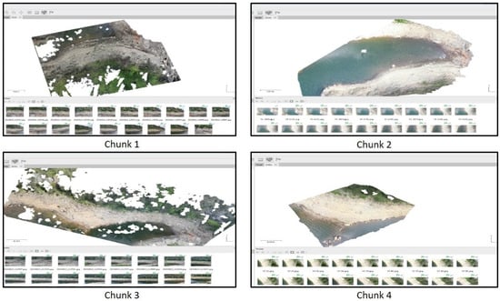
Figure 5.
Area covered by each of the four datasets through the processing of data using Agisoft Metashape© software.
Thus, to achieve a single model by merging the four datasets as shown in (Figure 6), a validation assessment in terms of the achieved error was performed in terms of each dataset separately (see Table 2). Moreover, it is necessary to guarantee an accurate merging to obtain a reliable single model. In this context, the final accuracy of the merged point clouding into a single one will be highlighted. All dataset processing methods were run by using the alignment tool following the standard workflow from Agisoft Metashape© software, consisting of the aero-triangulation and in the reconstruction of the dense point cloud. Starting from the first dataset, three GCPs were presented (numbered as 8, 9 and 11), additionally to one Check Point (CP), numbered as 10. The obtained accuracy can be evaluated depending on the obtained error related the check point. The error related to the first dataset is equivalent to 1 cm. Three GCPs (numbered 6, 7 and 11) and one CP (numbered as 10) were accessible in the second dataset. At present the error on CP (numbered 10) is around 5 mm. Furthermore, four GCPs (numbered 5, 7, 8 and 9) and one CP (numbered 6) were present in the third dataset; this leads to obtaining more reliable results. The achieved outcome of dataset 3 is similar to the first chunk and is equivalent to 1 cm. In case of the fourth dataset, and like the first and second chunks, three GCPs (2, 3 and 5) and one CP (point 4) were obtained. The error on CP was in a millimeter order of magnitude, similar to the second dataset, which was around 2 mm as reported in Table 2.
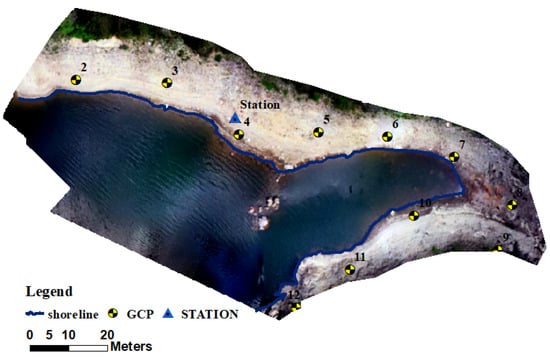
Figure 6.
An orthophoto representing the merged point clouds in a single one.
Table 2.
GCPs and CP error over each dataset. Tables are ordered consecutively (datasets 1–4) from top to bottom. The coordinates are provided in WGS84/UTM32N. The errors are computed by Agisoft Metashape based on bundle block adjustment.
After the results were obtained for each dataset separately, they were merged based on the GCPs positions. Using this method, the software calculated the estimated error on the selected CP, providing an accuracy estimation, conditionally on the GCPs coordinates. The merged four datasets turned into a single dataset, thus in a single point cloud. Ten markers (GCPs 2–11) were allocated as eight GCPs (2–5, 7, 8, 10 and 11) and two CPs (6 and 9) in order to validate the result in terms of the final merged point cloud. Highlighting that in dataset 4, only one common GCP (point 5) is in common with the other datasets, natural common points were considered in this case in the merging process. Overall, the obtained result of the merged point cloud had a representative error in terms of CPs equivalent to 4 cm, as shown in Table 3.
Table 3.
GCPs in the merged point cloud and final error in correspondence with the CPs. The coordinates are expressed in WGS84/UTM32N.
Afterwards, the merged point cloud elaboration allowed us to obtain an orthophoto with 2 cm/pixel resolution, which can be useful for the evaluation and visual analysis of topographic area. The orthophoto generation was the last step of the workflow using the Agisoft Metashape© software. All points are imported to GIS with the obtained orthophoto. The measured GCPs and the markers shown by the georeferenced orthophoto fit each other perfectly. The points that represent the zero-surface level, i.e., the points along the shoreline that define the real water level with respect to land, were also imported to the GIS. These points are extracted from the digitized shoreline of the lake. The zero-level points that are distributed along the shoreline in the study area are the base of the continuous interpolation surface between the emerged and submerged areas. Forty-one points are displayed in Figure 7 below, which represent the zero-level point.
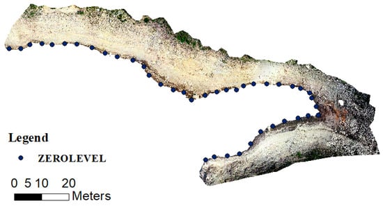
Figure 7.
Orthophoto obtained from digital photogrammetric images elaboration. The black dots represent the points along the shoreline, i.e., zero-level.
After importing the orthophoto and the dense cloud obtained previously to GIS, a topographic DSM was built. The results are shown in Figure 8a. As shown, the topographic area is divided into several colors representing a range of elevation values, from blue (as lower elevation) to red (as the highest elevation). Obviously, these ranges contain many outliers and noise that must be filtered out. Knowing that this DSM is related to the topographic area that is above both the real water level and the reference zero levels, all the points measurements having an elevation value less than zero must be eliminated. Moreover, as shown in the legend of the DSM, there are also height ranges between 8 and 30 m, and this is because of the presence of high trees in the outer boundary of the study area that influence the obtained DSM. Hence, after eliminating these points, for the emerged zone, the overall result is a DSM ranging from the water surface level (0 m) to 8.7 m as shown in Figure 8b.
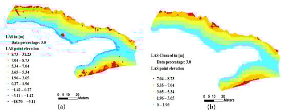
Figure 8.
DSM of the emerged zone. In (a), outliers are represented in red color close to the outer boundary of the study area, while (b) represents the emerged zone after filtering and cleaning noises to obtain a more reliable elevation range starting from the shoreline, thus obtaining a DSM ranging from zero to 8.75 m.
3.3. Bathymetric Data
The synchronization in time between the acoustic sensor and the GNSS receiver provides distance measurements related to real world position. The measured points coordinates were expressed in terms of latitude and longitude in WGS84, while the heights were represented in terms of measured distances between the SBES and ground at nadir. Knowing that the position of GNSS and SBES mounted on SWAMP have different locations, bathymetric data computation was performed, taking into account a common reference frame for sensors on the SWAMP vehicle (Figure 9).
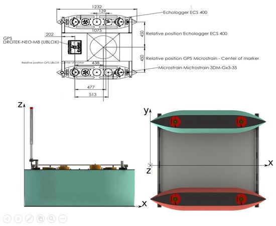
Figure 9.
SWAMP reference frame with the dimensions of the sensor located on the platform.
Ninety two thousand, three hundred and sixty nine bathymetric point measurements were shifted from the initial position to the new reference frame related to the SBES position. The first step was to project measurements from WGS 84 to WGS 84/UTM zone 32N. Subsequently, the obtained coordinates were shifted depending on the angular and distance difference between sensors mounted on the SWAMP. This step was followed by computing the shifted X and shifted Y from the GPS sensor position to the SBES position taking into consideration the orientation of SWAMP from the North. In this context, four quadrants were allocated, and depending on the presence of SWAMP in one of them, the shifted X and Y were calculated as shown in Table 4, where and represent the shifts along X and Y axes, respectively.
Table 4.
Equations to compute the shifts on X and Y axes taking into consideration the orientation of SWAMP with respect to the real North. d and j represent the difference in distance between the GPS antenna position and acoustic sensor and the orientation of SWAMP from North, respectively.
It is necessary to underline that the distance measurements compensated for the roll and pitch effects that were provided by the MU (Motion Sensor) mounted on the SWAMP.
Having a correct and accurate position for measurements is not enough. An essential step related to distance measurements correction must be considered. As previously clarified, elevations were taken on the basis of water level, and to achieve the continuity between emerged and submerged zones, it was necessary for the bathymetric and topographic measurements to have the same reference system, i.e., the water level. Knowing that the acoustic sensor is above the SWAMP bottom basements by 8 mm, and the SWAMP is immersed in water by 140 mm, then all measurements must be added to a value equal to 0.132 m. Thus, is the corrected distance between the water level and the bottom of the lake. The computed coordinates , , , , are provided in Table 5.
Table 5.
Computed , , . The coordinates are expressed in WGS84/UTM32N and account for both the distance between the GPS and SBES sensors mounted on the SWAMP along X and Y axes and the distance between GNSS and acoustic sensor positions along the Z axis.
The acquired bathymetric data are represented by colors ranging from light blue to dark blue, according to the increasing energy of the refracted acoustics signal. A lighter blue represents deep water, whereas a darker blue is used to display shallower areas, where the intensity of the refracted acoustic signal is higher. So, from Figure 10, an initial idea for the variation of depths over the study area could be noticed, depending on the color range of the points measurements.
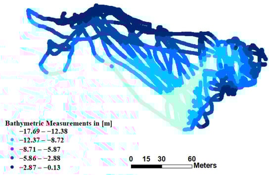
Figure 10.
Bathymetric points measurements with color intensity variation representing the distance with respect to the sensor: lighter color stands for higher depth (lower intensity of refracted acoustic signal) and darker color represent swallow water, where the intensity of acoustic signal refraction is higher.
3.4. Topographic/Bathymetric Data Integration Model
After showing the results for topographic and bathymetric data separately, the data are merged together on the basis of the calculated control points and the digitized shoreline between the two data sets. Data merging is performed by using a dedicated tool in GIS that provides a single continuous model. As previously described, the merging operation is carried out with respect to the same horizontal and vertical reference frame and taking into account the water level as the zero level for the elevation determination; furthermore, the dense point cloud has been used to represent the topographic area highlighted in brown (Figure 11). The used dense cloud has been filtered by deleting those outer limits defined as noise. Close to the shoreline, the color of the points is light brown, standing for low elevation values. The shoreline overlaps perfectly between the emerged and submerged area. The results are displayed in Figure 11 and show the merged datasets and the topographic and bathymetric measurements. This is the first step to obtaining a common continuous model of both environments.
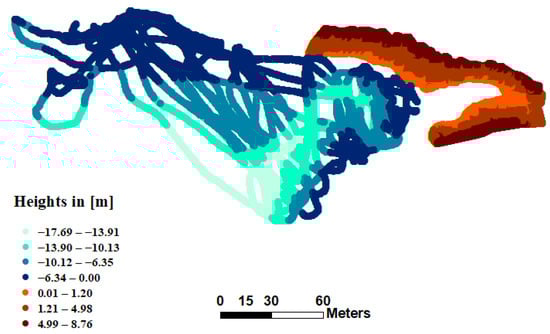
Figure 11.
Merged measurements including topographic and bathymetric data.
After merging the data, the last step to obtain the DSM is to interpolate the data depending on the elevation measurements. As already stated, among several interpolation methods, the Natural Neighbor interpolation has been considered one of the most suitable methods for these scattered data. Since SBES is used, it is essential to guarantee, through the interpolation, being within the range of the samples used. Hence, Natural Neighbor interpolation was used knowing that it does not infer trends nor produce peaks or valleys that are not already represented by the input samples. Natural Neighbor interpolation seeks to find the closest sample point to a query point and assign weights to each based on polygon proportionate areas around each point. The results of the obtained DSM from the Natural Neighbor interpolation with a resolution of (5 × 5 cm), shown in Figure 12, range between −17.68 m for maximum depth and 8.76 m as the maximum height from the water level.
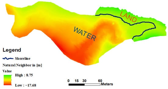
Figure 12.
Resulting DSM based on Natural Neighbor interpolation for the entire environment.
Through this range the model is reliable due to the fact that the Natural Neighbor criterion, unlike other tools, does not infer trends nor produce virtual peaks, ridges or valleys that are not already represented by the input samples. The surface passes through the sampled points and smooths the areas in between.
3.5. 3D Model and Volume Evaluation
By using the GIS 3D analyst application GIS environment [26] for overlaying several layers of data in the 3D model, a clearer visualization was obtained. Physical features are located in 3D by providing height information from feature attributes, feature geometry, a defined 3D surface, and every layer in the 3D view can be modified differently. Data are displayed based on relative coordinates positions or, in the case where different references occurred, all data are projected to a common projection. The 3D model built in ArcScene, depending on the obtained DSM, is represented by slightly different colors, which are related to the different elevation values. As shown in Figure 13a, the model represents the real shape of the study area, joining emerged and submerged portions. Under the water level, the ground is depicted from white to green to yellow, while above water level, it ranges from yellow to red to brown. An animation was created to show the real water level depending on this model (Figure 13b). Moreover, the volume of water is calculated, referring to the real water level measured through the survey campaign and this will be useful for future work. By achieving several survey campaigns for the same area, comparison and analysis could be performed in order to monitor the differences in morphology, water flow and variation in water volume.
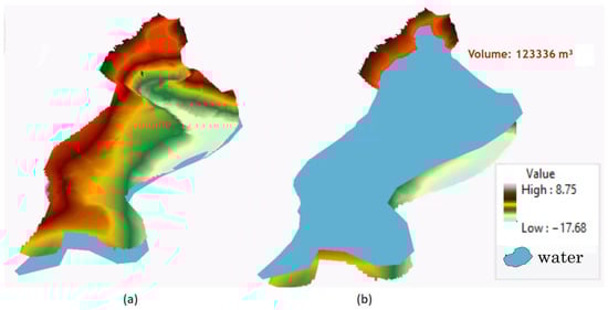
Figure 13.
Three dimensional (3D) model for rendering visualization analysis; (a) shows the geomorphology of the entire merged area, while (b) shows the results of water flow modeling and water volume determination.
4. Discussion
In this study, the development of surveying methodology for joint emerged and submerged environments was presented, treating a survey application combining an optical photogrammetric sensor, an SBES and a total station. Digital photogrammetry is low-cost and provides a huge amount of collected data in a reasonable amount of time. Furthermore, this source has been employed in order to obtain a final point cloud and an orthophoto for the terrestrial zone comparable with the expected centimetric accuracy. This was clearly highlighted in the provided results after data elaboration using Agisoft Metashape© software. The error outcomes related to all image datasets did not exceed a few centimeters and in some cases, it was even provided in millimeters.. Pertinently, the results are correlated with good GCPs distribution and the processing capabilities of the operators. Indeed, traditional techniques, such as the total station, require a high investment of human efforts; conversely, it is a worthy alternative with better accuracy than GNSS and without limitations on its use in the case of signal interference. Due to the unstable functioning of GNSS at the analyzed site, the total station made a fundamental contribution by achieving an accurate and reliable merging of datasets between emerged and submerged environments. After successfully merging data, a seamless and continuous DSM was obtained, starting from bathymetric and topographic data. It has to be considered that SBES is a low cost technique compared to others addressed to achieve bathymetric measurements, but it represents a good starting point in a steady environment such as a lake. Moreover, future steps can be performed to enhance the quality of the survey outcomes. Focusing on modifying the sensor locations mounted on SWAMP to set them in the same position, it will ease the calculation and avoid some systematic errors contributing to achieving higher standards with less efforts. Additionally, involving MBES instead of SBES could give extended opportunities for a wider underwater inspection range working with a higher accuracy, achieving higher standards in terms of IHO considerations and providing the ability for back scatter analysis and seabed classification. This will enhance the performance and the final products of the survey campaigns and provide the ability to have an analytical process for the sea bed. Moreover, the methodology will be developed by moving to the automatic markers detection for the photogrammetric survey and on the other side by considering SWAMP as a kinematic GCP with respect to the UAV to link both datasets from different environments in a smarter manner.
5. Conclusions
The present work aims to deepen different aspects of topographic and bathymetric techniques, to plan operations with an interdisciplinary approach, to develop methods for an integrated survey, to process different types of data, to analyze the obtained results and to generate an accurate graphic representation of a certain physical surface of the terrain. Particular attention has been paid to the differences between onshore topographic survey techniques and offshore bathymetric ones. In this context, a dedicated survey campaign was successfully carried out relying on SBES mounted on SWAMP ASV for bathymetric data collection and UAV and terrestrial photogrammetry for topographic survey. Bathymetric data was processed and georeferenced relying on GPS depending on identifying a common reference frame for all sensors mounted on SWAMP. The final output coming from bathymetric measurements was a georeferenced point cloud representing the depth measurements. On the other hand, photogrammetric data were georeferenced depending on GCPs measured by the total station. The integrated aerial and underwater survey campaigns provide a final point cloud and an orthophoto with a resolution of 2 cm per pixel. The results also showed the successful and accurate merging for the entire environment (emerged and submerged zones) depending on control points and the detected shoreline. The obtained continuous and seamless DSM was achieved by performing Natural Neighbor Interpolation between the two datasets. The obtained DSM was useful for extracting parameters for geomorphology, modeling water flow, rendering of 3D visualization and water volume determination. Finally, the interdisciplinary approach contributes to improving information quality, especially where there is no easy access. In other words, the interdisciplinary approach involving robotics and geomatics technologies enables us to work in a smarter manner, reducing the costs and extending the survey coverage and standards.
Author Contributions
Conceptualization, A.A.K., A.O., M.C. and D.S.; methodology, M.C. and D.S.; data collection: A.A.K., A.O. and M.B.; analysis and interpretation of results: A.A.K.; draft manuscript preparation: A.A.K., S.G., I.F., M.B., M.C., A.O. and D.S. All authors reviewed the results and approved the final version of the manuscript.
Funding
This research received no external funding.
Institutional Review Board Statement
Not applicable.
Informed Consent Statement
Not applicable.
Data Availability Statement
The data can be made available upon reasonable request.
Conflicts of Interest
The authors declare no conflict of interest.
References
- Salameh, E.; Frappart, F.; Almar, R.; Baptista, P.; Heygster, G.; Lubac, B.; Raucoules, D.; Almeida, L.P.; Bergsma, E.W.; Capo, S.; et al. Monitoring beach topography and nearshore bathymetry using spaceborne remote sensing: A review. Remote Sens. 2019, 11, 2212. [Google Scholar] [CrossRef]
- Xie, H.; Wang, H.; Yang, Y.; Chen, Y.; Yang, J.; Wang, S.; Liu, Z. Analysis of Underwater Topographic Survey of Stilling Basin Based on Unmanned Survey System. Adv. Mater. Sci. Eng. 2021, 2021, 5514165. [Google Scholar] [CrossRef]
- Alvarez, L.V.; Moreno, H.A.; Segales, A.R.; Pham, T.G.; Pillar-Little, E.A.; Chilson, P.B. Merging unmanned aerial systems (UAS) imagery and echo soundings with an adaptive sampling technique for bathymetric surveys. Remote Sens. 2018, 10, 1362. [Google Scholar] [CrossRef]
- Specht, C.; Lewicka, O.; Specht, M.; Dąbrowski, P.; Burdziakowski, P. Methodology for carrying out measurements of the tombolo geomorphic landform using unmanned aerial and surface vehicles near Sopot Pier, Poland. J. Mar. Sci. Eng. 2020, 8, 384. [Google Scholar] [CrossRef]
- Burdziakowski, P.; Specht, C.; Dabrowski, P.S.; Specht, M.; Lewicka, O.; Makar, A. Using UAV photogrammetry to analyse changes in the coastal zone based on the sopot tombolo (Salient) measurement project. Sensors 2020, 20, 4000. [Google Scholar] [CrossRef] [PubMed]
- Lubczonek, J.; Kazimierski, W.; Zaniewicz, G.; Lacka, M. Methodology for combining data acquired by unmanned surface and aerial vehicles to create digital bathymetric models in shallow and ultra-shallow waters. Remote Sens. 2021, 14, 105. [Google Scholar] [CrossRef]
- Gonçalves, J.A.; Bastos, L.; Pinho, J.; Granja, H. Digital aerial photography to monitor changes in coastal areas based on direct georeferencing. In Proceedings of the 5th EARSeL Workshop on Remote Sensing of the Coastal Zone, Prague, Czech Republic, 1–3 June 2011; pp. 1–3. [Google Scholar]
- Matias, M.P.; Falcão, A.P.; Gonçalves, A.B.; Alvares, T.; Pestana, R.; Van Zeller, E.; Rodrigues, V.; Heleno, S. A methodology to generate a digital elevation model by combining topographic and bathymetric data in fluvial environments. In Proceedings of the ESA Living Planet Symposium, Edinburgh, UK, 9–13 September 2013; Volume 13. [Google Scholar]
- Lewicka, O.; Specht, M.; Stateczny, A.; Specht, C.; Brčić, D.; Jugović, A.; Widźgowski, S.; Wiśniewska, M. Analysis of GNSS, Hydroacoustic and Optoelectronic Data Integration Methods Used in Hydrography. Sensors 2021, 21, 7831. [Google Scholar] [CrossRef] [PubMed]
- Dąbrowski, P.S.; Specht, C.; Specht, M.; Burdziakowski, P.; Makar, A.; Lewicka, O. Integration of multi-source geospatial data from GNSS receivers, terrestrial laser scanners, and unmanned aerial vehicles. Can. J. Remote Sens. 2021, 47, 621–634. [Google Scholar] [CrossRef]
- Gesch, D.; Wilson, R. Development of a seamless multisource topographic/bathymetric elevation model of Tampa Bay. Mar. Technol. Soc. J. 2002, 35, 58–64. [Google Scholar] [CrossRef][Green Version]
- Arseni, M.; Voiculescu, M.; Georgescu, L.P.; Iticescu, C.; Rosu, A. Testing different interpolation methods based on single beam echosounder river surveying. Case study: Siret River. ISPRS Int. J. Geo-Inf. 2019, 8, 507. [Google Scholar] [CrossRef]
- Quadros, N.; Collier, P.; Fraser, C. Integration of bathymetric and topographic LiDAR: A preliminary investigation. Int. Arch. Photogramm. Remote Sens. Spat. Inf. Sci. 2008, 36, 1299–1304. [Google Scholar]
- Włodarczyk-Sielicka, M.; Bodus-Olkowska, I.; Łącka, M. The process of modelling the elevation surface of a coastal area using the fusion of spatial data from different sensors. Oceanologia 2022, 64, 22–34. [Google Scholar] [CrossRef]
- Lucarelli, A.; Brandolini, P.; Corradi, N.; De Laurentiis, L.; Federici, B.; Ferrando, I.; Lanzone, A.; Sguerso, D. Potentialities of integrated 3D surveys applied to maritime infrastructures and to the study of morphological/sedimentary dynamics of the seabed. In Proceedings of the IMEKO TC-19 International Workshop on Metrology for the Sea, Genoa, Italy, 3–5 October 2019; pp. 3–5. [Google Scholar]
- Slocum, R.; Wright, W.; Parrish, C.; Costa, B.; Sharr, M.; Battista, T. Guidelines for Bathymetric Mapping and Orthoimage Generation using sUAS and SfM, An Approach for Conducting Nearshore Coastal Mapping; NOAA Technical Memorandum NOS NCCOS 265; National Oceanic and Atmospheric Administration: Silver Spring, MD, USA, 2019.
- Odetti, A.; Bruzzone, G.; Altosole, M.; Viviani, M.; Caccia, M. SWAMP, an Autonomous Surface Vehicle expressly designed for extremely shallow waters. Ocean. Eng. 2020, 216, 108205. [Google Scholar] [CrossRef]
- Odetti, A.; Altosole, M.; Bruzzone, G.; Caccia, M.; Viviani, M. Design and Construction of a Modular Pump-Jet Thruster for Autonomous Surface Vehicle Operations in Extremely Shallow Water. J. Mar. Sci. Eng. 2019, 7, 222. [Google Scholar] [CrossRef]
- Dinehart, R. Bedform movement recorded by sequential single-beam surveys in tidal rivers. J. Hydrol. 2002, 258, 25–39. [Google Scholar] [CrossRef]
- Chen, B.; Yang, Y.; Wen, H.; Ruan, H.; Zhou, Z.; Luo, K.; Zhong, F. High-resolution monitoring of beach topography and its change using unmanned aerial vehicle imagery. Ocean. Coast. Manag. 2018, 160, 103–116. [Google Scholar] [CrossRef]
- IHO Standards. 2021. Available online: https://iho.int/uploads/user/pubs/standards/s-44/S-44_Edition_6.0.0_EN.pdf (accessed on 4 April 2022).
- Agisoft Metashape©. 2021. Available online: https://www.agisoft.com (accessed on 20 December 2021).
- Federici, B.; Corradi, N.; Ferrando, I.; Sguerso, D.; Lucarelli, A.; Guida, S.; Brandolini, P. Remote sensing techniques applied to geomorphological mapping of rocky coast: The case study of Gallinara Island (Western Liguria, Italy). Eur. J. Remote Sens. 2019, 52, 123–136. [Google Scholar] [CrossRef]
- Turner, I.L.; Harley, M.D.; Drummond, C.D. UAVs for coastal surveying. Coast. Eng. 2016, 114, 19–24. [Google Scholar] [CrossRef]
- Autodesk©AutoCAD. 2021. Available online: https://images.autodesk.com (accessed on 4 April 2022).
- Geographic Information System (GIS)©. Available online: https://www.esri.com (accessed on 4 April 2022).
- Sierrasoft Topko. 2011. Available online: https://www.sierrasoft.com (accessed on 1 April 2022).
Publisher’s Note: MDPI stays neutral with regard to jurisdictional claims in published maps and institutional affiliations. |
© 2022 by the authors. Licensee MDPI, Basel, Switzerland. This article is an open access article distributed under the terms and conditions of the Creative Commons Attribution (CC BY) license (https://creativecommons.org/licenses/by/4.0/).