Characterizing Rogue Waves at the Entrance of Tampa Bay (Florida, USA)

Abstract

Rogue waves are a recognized but not fully comprehended hazard of major concern to the maritime industry. There is not one agreed-upon unified model that explains the formation of such waves and little is known about their frequency of occurrence. This study used in situ data from a wave buoy located at the entrance of Tampa Bay, Florida, to assess conditions that could lead to the development of these potentially destructive waves. Tampa Bay is a major commercial and transportation hub on the east coast of the United States. Wave buoy data from 2015 to 2019 were analyzed in this study. While more than 7000 individual waves that significantly exceeded median values were recorded, only 32 exceeded 4 m, thereby imposing risks to local navigation. The largest rogue wave that was recorded was 8.46 m high. Parameters in the time and frequency domains were calculated, local wind and surface current data were correlated, satellite synthetic-aperture radar (SAR) and vessel traffic data were analyzed, and the local bathymetry was considered. Based on our results, the narrow directional wave spreading that was found on the selected rogue waves was recognized as an important indicator of extreme waves. The parameters: surface elevation kurtosis, Benjamin–Feir Index (BFI), wave steepness, broadness, and narrowness factors, wind speed and direction, can be considered together, as a part of a local extreme-wave warning package. The selected individual rogue waves could not be identified using SAR imagery. Regional disturbances from ship wakes were analyzed but yielded no connections to the local formation of rogue waves.

1. Introduction

The term “rogue wave” is a relative concept. Rogue waves, also known as freak waves, are generally considered to be very large in relation to the associated wave environment. They are unpredicted waves that can occur either in the open ocean or in coastal waters. A rogue wave is commonly characterized as a wave whose maximum height (H_max) exceeds the value of twice the significant wave height (H_s). H_max indicates the zero-crossing maximum wave height and H_s is defined as the mean wave height (trough to crest) of the highest third of the waves in the wave spectrum, which is usually calculated from a 20- to 30-min measurement of surface elevation [1,2,3,4]. This is a practical statistical definition that assumes that the ocean wave height distribution is Gaussian, i.e., a value of less than two times the significant wave height corresponds to 95% of sea surface variability. This traditional concept does not convey the uniqueness and danger of rogue waves as it does not include a height threshold or other related physical parameters.

Rogue waves pose a significant danger to vessels and marine facilities. Many ship accidents, from damage to disappearances, have been reported that were likely related to rogue waves [5]; although most of these were not described as such, but rather it was inferred from accounts. The recognition of the hazards that are associated with extreme waves has increased in recent years, mainly due to incidents of waves striking passenger ships and platforms (e.g., the Draupner in 1995, the Queen Elisabeth II in 1995, the Caledonia Star and Bremen in 2000, the Explorer, Voyager and Norwegian Dawn in 2005, the Louis Majesty in 2010 and the MS Marco Polo in 2014), some of which resulted in fatalities [6,7,8]. The Draupner wave in 1995 was the first rogue wave to be recorded by sensors at a gas platform in the North Sea. As rogue waves are so costly, both in lives and economic impact, the maritime industry must consider the effects of rogue waves when designing large vessels [9,10,11,12,13].

Didenkulova (2020) compiled catalogue of 210 rogue waves that occurred worldwide from 2011–2018, which caused damages or even deaths. Most events were based on witness reports in the media and since there is very little wave sensor measurement in the ocean, these reports should be considered and provide an estimate of at least 20 to 30 rogue waves per year. The number of observations was much greater in coastal areas and in English speaking locations, which shows the bias of information that comes from more populated areas and from countries where information is easier to access. We can infer from this that the real number of rogue waves worldwide is much larger [14].

While research is continuing to better understand why, when and how rogue waves occur in the ocean, relatively few studies have utilized in situ wave data. The emphasis has been on understanding the physics behind rogue waves and determining environmental conditions in which waves could occur using mathematical models and water tank analyses [15]. The understanding of wave dynamics has mostly come from numerical models that were designed as simplifications of the equations that describe essential aspects of the event [16]. These approximations can be limiting when studying rogue waves because these events behave as outliers from statistical approaches.

Previous studies have linked the formation of rogue waves to both linear mechanisms (such as the overlapping of waves/focusing, dispersion enhancement, countercurrents and bathymetry) and nonlinear mechanisms (such as modulation instability and nonlinear focusing) [6,13,17]. Nonlinearity modifies focusing interactions due to the phase relations between spectral components, but it does not destroy them [18,19,20]. One hypothesis for rogue wave formation that was suggested by nonlinear theory is modulational instability, as measured using the Benjamin–Feir index [21,22]. However, the mechanisms that generate rogue waves remain uncertain. The relevant environmental parameters and characteristics of rogue waves include seasonality, directional spreading, surface elevation kurtosis, Benjamin–Feir index (BFI), wave steepness, wind data and ship wake information. Rogue wave characteristics are challenging to generalize because their behavior appears to depend on the bathymetry, currents, winds and wave directional spread at the location, as well as several other location-specific factors [23].

A few studies have used observed wave buoy data to identify parameters that can help to predict sea states that are more prone to rogue events. Baschek and Imai (2011) analyzed data from 16 buoys located along the west coast of the US to estimate the likelihood of rogue wave occurrence [1]. Cattrell et al. (2018) searched data from 80 buoys for specific parameters that could predict rogue waves [23]. Orzech and Wang (2020) examined data from 34 buoys and attempted to connect certain environmental factors with the development of rogue waves [22]. In the most recent study, Hafner et al. (2021) investigated the data of all 158 CDIP buoys and found that crest–trough correlation may help to generally forecast rogue wave formation [24]. Nevertheless, the detailed investigation of local sea and atmospheric conditions that could boost the development of rogue waves in one specific location has not been the focus of most analyses of rogue waves. Comparing the wave buoy results to Sentinel-1 SAR satellite observations [25,26], as well as an ERA5 reanalysis of wind data [27] and surface current information [28,29,30], has provided insight into the attributes of rogue waves that occur locally.

The study site was the entrance to the port of Tampa, FL, USA, in the eastern Gulf of Mexico (Figure 1). This port is the largest in the area and is the most diversified in Florida. Ranking 22nd in the nation in terms of tonnage [31], the port annually generates an economic impact of more than USD 15.1 billion and supports more than 80,000 jobs [32]. The Tampa Bay region includes the main cities of Tampa, St. Petersburg and Clearwater, making it the 18th largest metropolitan area in the United States with an estimated population of over 3,000,000 people. Every year, there are approximately 8000 large vessel transits in Tampa Bay in addition to thousands of smaller commercial, government agency and recreational vessels. The entrance to Tampa Bay can be affected by heavy storms and hurricanes, as well as by vessel wakes. Understanding how and when rogue waves are formed in one location would allow vessels to be warned about when such events are prone to occur [33,34]. Enhanced prediction can support better planning by the maritime industry and the safer execution of local operations and can be used to improve vessel design criteria [35].

This study focused on analyzing the relevant environmental parameters and characteristics of rogue waves, such as seasonality, directional spreading, surface elevation kurtosis, Benjamin–Feir Index (BFI), wave steepness, wind data and ship wake information, using a previously unexamined set of wave data to enhance the knowledge of what contributes to their development. The methods for detecting and characterizing the development of rogue waves were reviewed and applied to Tampa Bay. We examined the main theories based on the mechanisms mentioned above (crossing seas, opposing currents and modulational instability), in addition to atmospheric forcing (high winds and meso-scale wind gusts), to explain rogue wave formation in the offshore region of Tampa Bay.

The primary objectives of this study were: (a) to quantify the occurrence probability of rogue waves at the entrance of Tampa Bay; (b) to discuss the importance of modulational instability and crossing seas conditions [20,36,37] in the development of local rogue waves; (c) to investigate the effects of environmental factors, including weather, seasonality, bathymetry and local currents, on rogue wave evolution; and (d) to identify possible key effective spectral parameters (directional wave spreading, wave peakedness and the Benjamin–Feir index (BFI)) for rogue wave prediction.

2. Materials and Methods

This study examined waves with abnormally large amplitudes (H) using a time series (2015–2019) of in situ data from a Datawell Waverider MK-III wave buoy that is located 16.7 km west of the Egmont Key lighthouse, near to the main shipping channel at the entrance of Tampa Bay and with roughly 13 m of water depth (Figure 1). The use of the conventional definition for a rogue wave, i.e., a wave that exceeds the value of twice the significant wave height (H > 2H_s), yielded thousands of instances during the study period. Most of these events did not pose a perceptible threat to navigation due to insufficient wave height. However, model studies have indicated that some vessels can capsize when an individual wave height reaches 30% of the hull length [38]. Waves higher than 4 m pose a threat to vessels that are < 15 m (49.2 ft) in length [39].

The wave buoy provides raw heave data as well as processed wave data, which is information that is indispensable for a rogue wave study. The buoy records waves with periods of between 1.6 s and 30 s and heights up to 40 m. The buoy data is sampled at 1.28 Hz (every 0.78125 s) for a total of 1600 s each half hour (~27 min), producing 2048 data points that are internally processed and transmitted during the remaining minutes of the half-hour cycle. The buoy displacement resolution is 0.01 m and its error is <3%. This buoy is maintained by both the University of South Florida and the Coastal Data Information Program (CDIP) from the Scripps Institution of Oceanography as part of a wave buoy array of approximately 80 buoys that are maintained by CDIP around the world and is a component of the NOAA Tampa Bay Physical Oceanographic Real-Time System (PORTS^®).

2.1. Data

CDIP buoys are among the few in the world that make available raw surface elevation data, which are essential for the calculation of maximum wave heights and, consequently, rogue waves. The surface elevation dataset is divided into half-hour sections, which is the transmission time between wave measurements. Individual waves were identified for this study via the zero-upcrossing method [40], which was used to calculate the maximum wave height (maximum vertical displacement within the half-hour period) and the significant wave height (H_s; the average of the highest third of the waves).

The H_s data were compared to the significant wave height data that were provided by the CDIP’s buoy data spectral processing software. The spectrally computed significant wave height was denoted H_m0 and was calculated as being equal to four times the square root of the first spectral moment (M₀) [41]. H_s was approximately 5% lower than H_m0 [3], as was also found using our calculations below.

Rogue waves are traditionally defined as occurring when the maximum wave height (H_max) exceeds the significant wave height (H_s) by at least a factor of two [3,6,42,43]. As this definition usually yields a large number of results, some studies have used other definitions, such as H_max/H_s ≥ 2.2 [44], H_max/H_s ≥ 2.3 [45] or the ratio of maximum crest height (C_max) to significant wave height of C_max/H_s > 1.25 [3,46]. The crest height is the highest point on a wave trace between the time it crosses above and below the mean water level. We also considered rogue holes and calculated the minimum trough height in relation to H_s; however, we decided not to include these data in the study because they did not yield significant (i.e., hazardous) results. The numbers of rogue waves that were found using the different definitions above can be found in

Table 1. The different definitions of rogue wave events and the number of waves that met those criteria that were found in the dataset recorded by the CDIP Waverider buoy near Egmont Key in 2015–2019. H_max is the measured maximum wave height (from maximum surface elevation), H_s is the significant wave height and C_max is the maximum crest height.

Type of Rogue Event	Number of Waves
Hmax/Hs > 2	7593
Hmax/Hs > 2.2	1821
Hmax/Hs > 3	99
Cmax/Hs > 1.25	2547
Hmax > 4.0	372
Hmax > 4.0 and Hmax/Hs > 2	32
Hmax > 4.0 and Hmax/Hs > 2.2	9
Hmax > 4.0 and Cmax/Hs > 1.25	29
Hmax > 4.0 and Cmax/Hs > 1.25 and Hmax/Hs > 2	17

. To focus our study on the rogue waves that could potentially cause damage to the maritime industry, we narrowed our threshold and only identified rogue waves that had H_max > 4 m and followed the traditional definition of H_max/H_s ≥ 2.0. In 2015–2019, the buoy, which had some sampling pauses due to necessary maintenance, collected a total of 72,646 individual wave events. Out of all of these waves, 7593 (more than 10%) were considered to be of abnormal height (height > 2H_s). However, from these abnormal waves, only 0.77% had heights exceeding 3.66 m (Figure 2). Other studies have mentioned the issue of the non-rareness of the occurrence of rogue waves when using the traditional definition criterion and, as in this study, have used additional constraints to capture their gravity, power and scarcity [1,22,23,24,47,48].

A post-process data quality control procedure (CDIP) marked the vertical displacement data with the following flags: good, questionable, bad or missing. Only the 30-min wave data that had “good” and “questionable” flags were considered. Although rogue waves could be considered as errors by the filtering process, discussions with CDIP personnel verified that extreme wave values are not flagged as “bad” data, even though they deviate quite strongly from the average surface elevation data.

2.2. Parameters

Wave data analyses that were performed both in the time domain and the frequency domain allowed for the identification of abnormally high waves and the calculation of parameters, such as time periods and the kurtosis values of the individual waves. The parameters in the frequency domain were calculated following the method of Orzech and Wang [23] and are summarized in

Table 2. A summary of the different wave parameters in the time and frequency domains that were analyzed in this paper, along with their descriptions and equations. Where σ is the standard deviation, M_o, M₁, M₂ and M₄ are the zeroth, first, second and forth spectral moments of the wave energy spectrum, respectively. K_p is the peak wave number, $\mathrm{a}$ is the amplitude (H_s/2) and the product ${\mathrm{K}}_{\mathrm{p}}\times \mathrm{a}$ is the wave steepness [22].

Frequency Domain Parameters
Hmo	$4\sqrt{{\mathrm{M}}_0}$	(1)
Wave Steepness	$2\times \mathsf{\pi }\times \frac{2\times \mathsf{\pi }\times {\mathrm{H}}_{{\mathrm{m}}_0}}{\mathrm{g}\times {\mathrm{T}}_{{\mathrm{m}}_{02}}^2}$	(2)
Broadness Factor (ε)	$\sqrt{(1-\frac{{\mathrm{M}}_2^2}{\left({\mathrm{M}}_0\times {\mathrm{M}}_4\right)}}$	(3)
Narrowness Factor (ν)	$\sqrt{\frac{{\mathrm{M}}_0\times {\mathrm{M}}_2}{{\mathrm{M}}_1^2}-1}$	(4)
Peakedness Factor (Qp)	$\frac{2}{\begin{array}{c}{\mathrm{M}}_0^2\\ \end{array}} {{\displaystyle \int }}_{\mathrm{L}\mathrm{F}}^{\mathrm{H}\mathrm{F}}\mathrm{f}{\left[\mathrm{s}\left(\mathrm{f}\right)\right]}^2 \mathrm{d}\mathrm{f}$	(5)
Irregularity Factor (α)	$\frac{{\mathrm{M}}_2}{\sqrt{\left({\mathrm{M}}_0\times {\mathrm{M}}_4\right)}}$	(6)
Benjamin–Feir Index (BFI)	$\sqrt{2} \left({\mathrm{K}}_{\mathrm{p}}\times \mathrm{a}\right)\times \left(\sqrt{\mathsf{\pi }} {\mathrm{Q}}_{\mathrm{p}}\right)$	(7)
Time Domain Parameters
Hs	The highest third of the waves
Hmax	Highest wave in the measuring period (30 min)
Wave Peak Direction	Direction in degrees from which the highest energy waves travel
Kurtosis	σ4 of surface elevation (heave) data

.

The first estimation of the spectral bandwidth is the broadness factor (ε), as defined by Cartwright and Longuet-Higgins in Equation (3) [49]. A wave spectrum is deemed to be narrow-banded when this broadness factor approaches zero. The second estimation is the narrowness factor (ν), as defined by Equation (4), which was first introduced by Longuet-Higgins in 1975 [50]. This parameter is used to define the width of a narrow spectrum. It is related to (ε), where ε = 1/2 ν in a narrow spectrum. The parameter alpha (α), defined by Equation (5), is the irregularity parameter of the width of the spectrum and is related to ε by $\mathsf{\alpha }=\sqrt{1-{\mathsf{\epsilon }}^2}$ [51]. Equation (6) presents the definition of the Goda’s peakedness parameter of the wave spectrum [52]. This parameter can also describe the statistics of run lengths, but it is sensitive to the resolution of the spectral analysis. Lastly, the Benjamin–Feir index (BFI), defined by Equation (7), describes the statistical properties of the surface elevation due to nonlinear instabilities. The BFI represents the ratio of the wave steepness to the spectral bandwidth, which is more pronounced when there is a larger deviation from a Gaussian distribution [53].

In addition to the statistical parameters and frequency domain factors that were calculated directly from the buoy data, we also used external data from different sources to compare to our results. Observed surface current data were acquired from the NOAA bottom-mounted Acoustic Doppler Current Profiler (ADCP), station ID t01010, which is located below the Sunshine Skyway Bridge (Figure 1). Modeled surface current data were calculated by the USF College of Marine Science Ocean Circulation Group, who developed and operate the WFCOM: a high-resolution numerical hydrodynamic model for the West Florida Shelf. Satellite SAR data were obtained from Germany’s Aerospace Center DLR (Deutsches Zentrum für Luft- und Raumfahrt). The DLR’s proprietary algorithm for characterizing sea state conditions by analyzing Sentinel-1 satellite SAR data (with spatial resolutions of down to 5 m and a swath of up to 400 km) was also used to check for rogue waves in the same time periods as those found by the buoy. Wind data, which were utilized to check for wind effects during the identified rogue events, were derived from the ECMWF (European Centre for Medium-Range Weather Forecasts) ERA5 reanalysis. This weather reanalysis is one of the most accurate in the world since it assimilates data from a large variety and quantity of sources. The wind data have a high spatial resolution (31 km) and cover the period from 1979 to the present. Finally, we also used local vessel traffic records from the Automatic Identification System (AIS) to check for the passage of large ships around the time of the identified rogue wave events in order to determine whether their wake could be related to local rogue wave formation.

3. Results and Discussion

3.1. Overall Buoy Data Analysis

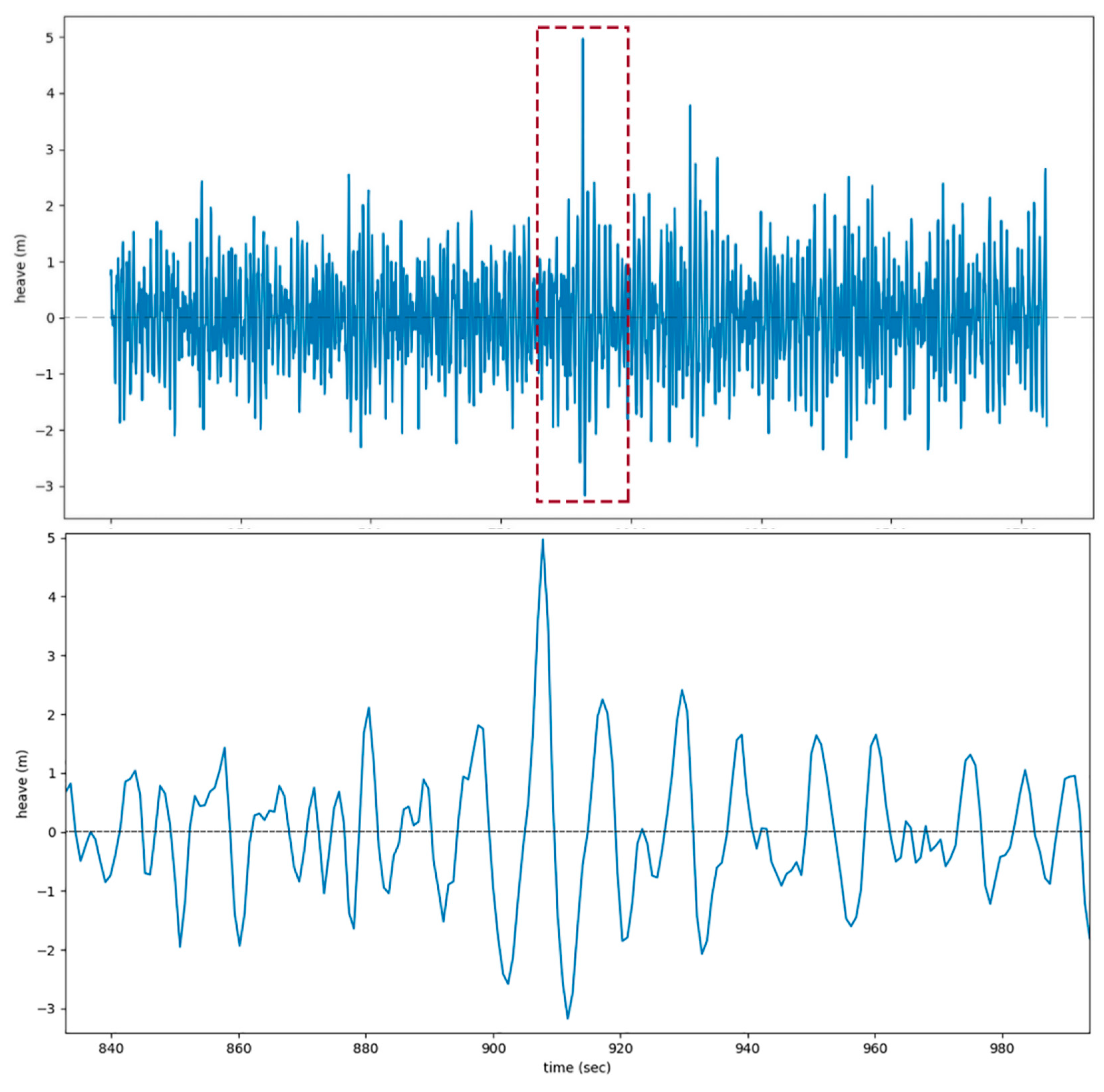
The Waverider buoy that was selected for this study has been monitoring wave characteristics since 2015. This study examined the 72,646 waves that were measured from 2015 until 6 December 2019 (there were some pauses due to equipment maintenance) and detected several rogue waves. An example of a rogue wave event that was measured on 23 January 2016 at ~10:33 UTC is shown in Figure 3.

As the location of the buoy is mainly protected by land to the east, we expected that the largest waves would come from the west (from 180° to 360°). Indeed, the highest waves came from a narrow directional spread of 245° to 295° (Figure 4).

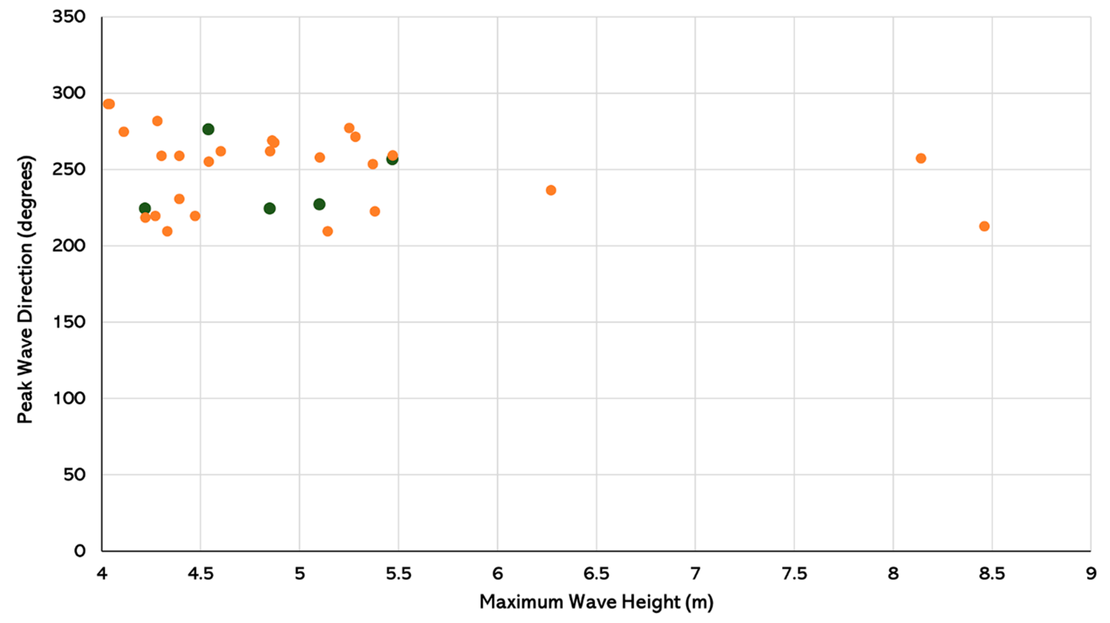
In Figure 4, the narrow wave directional spreading for the higher H_s values can be noticed. The peak direction of the 32 selected rogue waves plotted against the maximum wave height (H_max) indicated that the directional spread of the rogue dataset was much narrower than that for all waves. These waves were clearly grouped between 200° to 300° and the higher, therefore more dangerous, rogue waves all came from 270° (Figure 5). This is an important result for the local characterization and prediction of rogue wave events.

The seasonality of rogue occurrences was another element that was considered. Most (75%) of the 32 rogue waves occurred between October and February, comprising late fall and winter months. During the winter, the difference between the amount of solar radiation reaching the poles and the equator is at its maximum and the resulting larger temperature difference intensifies atmospheric circulation patterns, leading to more storms and stronger winds, which usually generate rougher seas conditions as well. These conditions support sea instability and the generation of rogue waves.

These results agreed well to those of Cattrell (2020), who found an increased rogue wave occurrence and rogue waves of higher severities in winter compared to summer [54]. Cattrell explained this phenomenon using the linear relationship between the rogue wave occurrence and height and the spectral bandwidth narrowness factor (ν). This study, on the other hand, instead found a closer relationship between the rogue wave occurrence and height and the spectral bandwidth broadness factor (ε). During colder months, the spectral bandwidth tends to be larger, which could cause the increase in rogue wave occurrence and height.

In contrast, Florida’s western continental shelf is highly prone to hurricanes during the hotter months from May to November and these events, when nearby, can also increase the instability of the ocean and support the development of rogue waves. Indeed, 4 rogue waves out of the 32 that we studies occurred on the same day (10 October 2018) and were probably generated by Hurricane Michael, which moved across the eastern Gulf from Yucatan in the direction of the Florida Panhandle to the west of Tampa Bay and made landfall as a category 5 event on that same day. From 9 October to 10 October, the hurricane’s increasing wind strength along its path, which passed to the west of the buoy, generated waves that were high enough to result in the formation of five rogue waves when in conjunction with a very unstable sea.

In conclusion, the seasonality of rogue waves at the entrance of Tampa Bay can be directly correlated to strong weather systems occurring nearby, both in warmer months and colder months. Since climate change is causing more extreme weather events, this may also support the development of more rogue waves.

3.2. Statistical Buoy Data Analysis

Based on previous studies, one of the first indicators of rogue wave events that we examined was that of surface elevation kurtosis (σ⁴). This statistical parameter measures the deviation between the sampled surface elevation distribution and a Gaussian distribution. Kurtosis is the standard deviation raised to the fourth power, which means that only data that are outliers contribute to an increase in the kurtosis values. When the kurtosis value was equal to three, the dataset followed a Gaussian distribution. Due to the nonlinear interactions, kurtosis values for waves are usually larger than three. The larger the kurtosis values, the longer the distribution’s tail and the more extreme the values that are present, i.e., the higher the kurtosis values, the higher the probability of rogue wave occurrence [9,55].

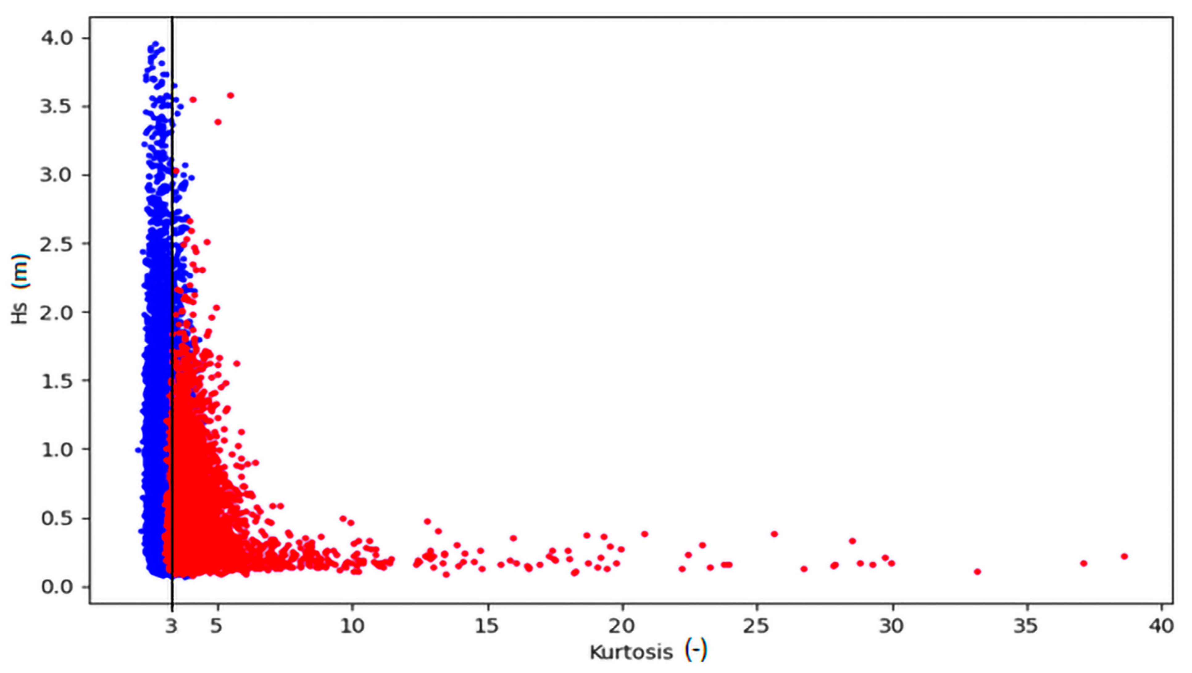
When the kurtosis values were plotted against the significant wave height values (Figure 6), the strong distribution around the kurtosis value of around three indicates that most of the waves did follow the Gaussian distribution. Rogue waves (any wave with H_max/H_s > 2) deviated from the Gaussian distribution. Rogue waves are more likely to occur for small values of significant wave height since higher kurtosis values (>6) are all related to low H_s (<1 m). The reason for this phenomenon is likely to be that it is more difficult to develop a rogue wave when the significant wave height is already high. The sea requires much more energy (i.e., more wind and other special conditions) to form higher waves than lower amplitude waves. Wave energy is proportional to the squared height, so waves need a quadratic growth of energy for the linear growth of wave height. Therefore, when the significant wave height is low, it is easier to create freak waves where H_max exceeds H_s by at least a factor of two [56]. Note also that extremely high kurtosis values (> 10) occur at very low H_s values (< 0.5 m). Considering two physically different types of waves, low waves (also short wavelength) are mainly wind waves. These waves are steep (mostly pyramid-shaped with a local surface slope of often > 20°) and have less spreading, so the abnormal waves (H_max > 2 H_s) can be created relatively often even by the usual collision of two such wind waves. However, waves of H_max > 4 m are mostly large swell waves or at least consist of 50% swell. These are longer waves with slopes of ~1–5°. Such waves require a stronger trigger to generate an abnormal wave.

In Figure 7, the two highest maximum wave heights that were measured indeed corresponded to higher kurtosis values; however, there was no overall correlation between the wave height and the kurtosis value. As shown in Figure 6, the kurtosis value was higher for rogue waves compared to non-rogue waves, which makes this parameter possible for use as a rogue wave indicator at the study location. The kurtosis values for the 32 highest rogue waves were all >3.4.

An overall statistical analysis of the wave values that were measured in each 30-min period produced the results in

Table 3. A simple statistical analysis of the 30-min averaged CDIP Egmont Key (FL, USA) buoy data from June 2015 to December 2019.

	Hs (m)	Hmax (m)
Mean	0.587	1.041
Variance	0.148	0.444
Std. deviation	0.384	0.666
Skewness	2.178	2.098
Kurtosis	8.097	7.63

. The kurtosis values were very high due to the large number of waves with low H_s, which generated comparatively higher waves more easily. Most H_s and H_max statistical results for this location were low, which means that it is relatively safe to navigate.

The probability density function (PDF) and the empirical cumulative density function (ECDF) of the 30-min averaged wave data are illustrated in Figure 8. The long tails revealed in the PDF distribution were the cause of the high kurtosis values. The probability of an abnormal wave using the traditional definition, H_max/H_s > 2, was also considered too high by the order of 10%. The probability of a maximum crest height (C_max) divided by H_s of more than 1.25 was also too high to be used as a rogue event definition. In 1952, Longuet-Higgins showed that random wave heights (H) follow the Rayleigh probability distribution [56]. The properties of the Rayleigh distribution indicate that:

$${\mathrm{H}}_{\mathrm{rms}}=4\times \mathsf{\sigma }$$

where σ is the standard deviation of the sea surface height variation.

$${\mathrm{H}}_{\mathrm{s}}=\sqrt{2 }\times {\mathrm{H}}_{\mathrm{rms}}=\sqrt{2}\times 4\times \mathsf{\sigma }$$

When the height of a rogue wave is ≥2 $\times$ H_s, then 2 $\times \sqrt{2}\times 4\mathsf{\sigma }$ ≥ 11.36σ and the amplitude of the rogue wave is ≥5.68σ. In a normal distribution (assuming waves in the ocean are normally distributed), we know that 2σ captures 95% of the sea variability; so, 5.68σ captures more than 99.99% of the sea height variability, which does not agree with our results or the results from broader studies [1,23,24,48]. This further indicates that wave parameters are not normally distributed and therefore, the rogue wave definition of H_max/H_s > 2 should be changed.

The ECDF represents the proportion or count of observations that fall below each unique value in a dataset in which the maximum is always 1.0 or 100%. The x-axis corresponds to the values of the plotted variable and the y-axis represents the proportion of data points that are less than or equal to the corresponding x-axis value.

3.3. Frequency Domain Analysis

The wave spectrum data for each of the averaged 30-min samplings were analyzed and the main spectral moments (M₀, M₁, M₂ and M₄) were derived to calculate the important parameters, including spectral significant wave height (Hm₀), wave steepness, narrowness factor (ν), broadness factor (ε), peakedness factor (Q_p), irregularity factor (α) and the Benjamin–Feir Index (BFI). These parameters are important for measuring the nonlinearity and instability of the wave systems as possible indicators of rogue waves; the local occurrence of such waves was compared to each of these parameters, as shown in Figure 9.

The Benjamin–Feir index BFI is basically the ratio between wave steepness and spectral bandwidth, as shown in Equation (5). The larger the BFI, the more pronounced the departure from the Rayleigh distribution [57,58]. This change in the distribution type is attributed to nonlinear modulation instability, which leads to highly erratic sea conditions (“rogue sea state”) that are characterized by a high concentration of unstable modes [59]. A high (≥1.0) BFI value is strongly associated with modulation instability, which can prompt rogue wave formation. The BFI values for most of the 32 rogue waves that were selected for our study (shown in red) fell between 0.5 and 1.0 (Figure 9a). A BFI value larger than 0.5 already shows a departure from the Rayleigh distribution; however, all sea state samples with H_m0 > 2 seem to follow this condition. Thus, BFI alone is not a useful parameter for identifying local rogue events, thereby indicating that these rogue events do not seem to be generated by modulation instability.

Similarly, significant spectral wave steepness (Figure 9b) is defined as the ratio between Hm₀ and deep-water wavelength, which corresponds to the Tm₀₂ wave period:

$$\mathrm{Significant} \mathrm{spectral} \mathrm{wave} \mathrm{steepness} = 2\times \mathsf{\pi }\times \frac{2\times \mathsf{\pi }\times {\mathrm{H}}_{{\mathrm{m}}_0}}{\mathrm{g}\times {\mathrm{T}}_{{\mathrm{m}}_{02}}^2}$$

where Tm₀₂ is the zero-crossing period = $2\times \mathsf{\pi }\times \sqrt{\frac{{\mathrm{M}}_0}{{\mathrm{M}}_2}}$ [60].

Some authors have used this parameter to classify waves as wind waves (0.08–0.025), young swell (0.025–0.01), mature swell (0.01–0.004) and old swell (< 0.004) [61].

Figure 9b indicates that the dispersion of the wave steepness data for the 32 selected rogue waves was consistent with all waves that satisfied H_m0 > 2. Although wave steepness is directly related to BFI, Figure 9b confirms the conclusions drawn from Figure 9a.

The broadness factor (ε), also called the spectral width parameter [62], was calculated using Equation (2) and the narrowness factor (ν) was calculated using Equation (1). When ε (Figure 9c) and ν (Figure 9d) approach zero, the energy is concentrated close to the peak frequency and the spectral bandwidth is narrow. When ε and ν approach one, the energy is dispersed over a wider range of frequencies and the spectral bandwidth is broad. According to Cattrell [23], the probability of a rogue event increases with higher ν values. Our rogue wave data matched the expected ν values for storm events, ranging from approximately 0.35 to 0.55. Our broadness factor (ε) data also showed that sea states with H_m0 > 2 had higher spectral widths, which was consistent with Cattrell’s findings [23]. Based on these results, we concluded that there is no need to consider these parameters separately for possible rogue wave identification since the rogue wave data are very similar to the normal sea state data. The critical parameter is simply the significant wave height.

The Goda’s peakedness parameter (Q_p) has been recognized as being an appropriate parameter to describe spectral distribution since it does not depend on the cut-off frequency, unlike ν and ε [63]. Q_p is considered to be a good indicator for spectral narrowness, with high values for narrowband spectra and low values for broadband spectra. Fully developed wind waves have Q ≈ 2, whereas narrow-banded swells have values of >2 [64]. Q_p is also intrinsically related to BFI [22]. As the waves become higher, the spectral peakedness parameter declines. Most of the selected rogue waves in our study had Q_p values of between 1.5 and 2.5 (Figure 9e).

The irregularity factor (α) is defined by the number of mean sea level zero-crossings divided by number of local maxima and indicates the number of peaks per wave; a smaller α indicates a more irregular sea state. This parameter, as with all of the others, seems to be more dependent on the wave height than any other value. Figure 9f confims that as waves become higher, they become more irregular (lower value of α).

All of these results agreed with those reported by Cattrell [23], indicating that the occurrences of the selected rogue waves were mainly independent of these spectral parameters and therefore, were not likely to be generated by nonlinear modulation instability.

3.4. Crossing Seas

Crossing sea states are characterized by two different wave systems, with different spectral peaks and propagation directions, crossing paths. Depending on the spectrum of each system and the angle at which they meet, this situation can increase nonlinear interactions, modulational instability and, consequently, rogue wave occurrence [18]. Based on numerical simulations, two wave systems with similar spectra that cross at about a 50° angle could generate a rogue wave.

To test these conditions with our data, we generated a polar plot of the wave system spectrum on the dates and times of the 32 rogue waves that were selected. We found 17 clear unimodal sea states and only 4 clear bimodal sea states. We found 11 sea states that we considered to be “mixed”, which showed various or indistinguishable pockets of energy in different directions. Rogue waves developed both in unimodal seas and bimodal seas that crossed at different angles. The Figure below depicts examples of rogue wave occurrence in a unimodal sea (Figure 10a), bimodal sea (Figure 10b) and a “mixed” sea (Figure 10c). These results further indicated that the rogue waves that were found at the entrance of Tampa Bay were not dependent on modulation instability.

Crest heights and wave lengths in a crossing sea state depend on the different frequencies of each system and the crossing angles, thus influencing the value of H_max. The result is almost the opposite of the effects of a nonlinear crossing sea, in which H_max is independent from spectral bandwidth and crossing angle. A previous study showed that the nonlinear effects of crossing seas are related to the average wave steepness, kurtosis values and the BFI [18].

3.5. Opposing Currents

Opposing currents occur when a surface current with a relatively high magnitude that is traveling in the opposite direction to the waves destabilizes the wave system. The presence of an opposing current creates a shift in the modulational instability band, which can trigger rogue waves. The probability of rogue wave occurrence increases with the strength of the opposing current [30]. This situation matters the most in locations with very high-velocity surface currents, for example, in the Gulf Stream or the Agulhas and Kuroshio currents, which may reach speeds of 1.5 m/s. Our studied location in the Gulf of Mexico, on the West Florida Shelf, does not have currents of these magnitudes and hence, the currents do not have the strength to influence local rogue wave formation.

To test this hypothesis, we collected surface current data from two different sources: (1) a high resolution (100–300 m) operational local circulation model of the West Florida Shelf (WFCOM) [65]; (2) a bottom-mounted ADCP located beneath the Sunshine Skyway Bridge, which crosses Tampa Bay and under which the shipping channel passes. The ADCP is mounted approximately 27 km to the east of the CDIP buoy, in a location that is much more sheltered from open sea currents.

The WFCOM circulation model started working from the second half of 2018, so we could not obtain data from this model for the time periods before that date. The data from the local ADCP were missing for several time periods, including the entire year of 2017. We were able to retrieve 11 points for surface current data from the WFCOM and 19 points from the ADCP. Since the direction that is recorded for the current is that in which it is heading and the direction that is recorded for waves is from which they are coming, the data must show similar values in order to be considered opposite. For the rogue waves for which we had current data, both wave and current direction values were similar for 12 of the rogue waves and were different for 7 of the rogue waves. The highest values for surface current velocities were ~0.75 m/s, which is about half of the velocity of the more dangerous previously mentioned currents, even during hurricane events. More work needs to be conducted in assessing local opposing currents since we did not have sufficient or reliable surface current data to draw firm conclusions; however, based on the current data that we could analyze, the surface current velocities are not high enough to be considered as a trigger for rogue wave formation.

3.6. Wind Data

It is still uncertain whether nonlinear interactions between waves are suppressed or amplified by high wind velocities. Laboratory experiments have produced highly variable results: the modulation instability of waves could be suppressed [66,67]), unaffected [68] and even enhanced [69,70]. Using experiments conducted in a large wind wave facility to study the effect of wind on waves [71], Lee and Monty confirmed that more wind energy increases the instant surface elevation values, thereby leading to exponentially higher significant wave height values. Larger waves induce higher wind-produced pressure drag forces, which results in waves reaching the breaking point faster. Although these experiments demonstrated an increase in wave amplitude modulation, they did not clarify the relationship between nonlinear interactions.

Orzech and Wang (2020) used the CFSR (NCEP Climate Forecast System Reanalysis) data to correlate rogue wave formation with wind speed and direction [22]. The CFSR wind data that were used had a resolution of approximately 50 km and did not contain information on either near-surface turbulence or wind gusts, which potentially affect wave growth. Their results suggested that very strong winds (≥ 23 m/s) coming from a similar direction to the waves may prevent rogue wave development, while moderately strong winds (≥ 10 m/s) coming from the opposite direction were found to be twice as strongly linked to rogue wave formation. However, they concluded that wind information provides very limited support for a causal connection between wind and rogue wave generation.

We extracted wind data for the exact location of the buoy from the ECMWF ERA5 reanalysis to compare to our wave data. The reanalysis comprises a number of meteorological and oceanographic data observations with past weather forecasts, which are globally complete without gaps. Observations include those from in situ sensors in weather stations, airplanes, radiosondes, vessels and buoys and remote sensing observations from satellites and ground-based radars. The reanalysis presents the most comprehensive picture of past weather conditions that is possible. ERA5 provides hourly estimates of several climate variables from air, land, and ocean. It covers the Earth with a 30 km grid and resolves the atmosphere using 137 levels from the surface up to a height of 80 km [72].

The cartesian components of the wind vectors from our chosen buoy location were extracted and then transformed into wind speed and direction data. The results showed a very weak positive correlation coefficient between wave height and wind speed (Figure 11a). The higher individual waves (H_max) presented a slightly stronger positive correlation of the highest waves to the highest winds. The rogue waves were related to wind speeds of more than 8.6 m/s and instantaneous wind gusts of more than 11.3 m/s. Seven rogue waves occurred during wind gusts of ~20 m/s or more and did not agree with Orzech and Wang’s results, which indicated that high winds could prevent rogue wave formation [22]. The wind and wave directions showed a strong correlation (Figure 11b). Wind directions that were associated with rogue waves came from 150° to 350° and rogue wave directions came from 200° to 300°. These results showed that the rogue waves that were analyzed were mainly not formed by wind–wave interactions that increased modulation instability.

We also compared the ERA5 wind data to a nearby NOAA station called MTB (Middle of Tampa Bay, ID: MTBF1-8726412), which is located about 34 km east of the Waverider buoy. Even though the MTB station is in a more protected area inside Tampa Bay, the wind speeds and directions were very similar between the two. As expected, the ERA5 had slightly higher values for wind speed and gusts most of the time (72%) since that buoy is in open sea (see Supplemental Table S1).

3.7. Satellite Synthetic-Aperture Radar (SAR) Data

Relatively new methods for estimating individual wave height with satellite Synthetic Aperture Radar (SAR) data [73] were developed in the MaxWave project. That project took place from 2000 to 2003, with goals that included establishing a better understanding of the properties of rogue waves and building risk maps and warning criteria [26]. These new methods enabled the observation of individual rogue waves using SAR from satellites for the first time. However, this technique has important limitations. Initially, they use linear assumptions to invert the radar information into a sea surface image. Furthermore, only wavelengths that are greater than about 100 m can be detected. From SAR data, the MaxWave project showed that rogue waves mostly appeared in prolonged storm systems or in crossing sea states [14]. This has also been confirmed by investigations using the Lloyd’s database of ship accidents. Toffoli et al. (2005) combined information about 200 ship accidents with wind and wave spectra data from WAM (wave model) and data from satellites [5]. They found that these accidents did not always occur in very heavy sea states and that crossing seas and rapidly changing wind conditions were more common.

Other research has continued to employ these techniques to derive sea state information from SAR Satellites after the MaxWave Project ended, especially the German Aerospace Center (DLR), which has published several papers [74,75,76] on the development of algorithms to correctly obtain sea state parameters from SAR satellite images. DLR’s algorithms can estimate integrated sea state parameters for different modes of the SAR satellite Sentinel-1 (S1). An empirical algorithm estimates H_S from SAR scenes using integrated image spectral parameters, as well as estimated local wind information and texture analysis based on gray level co-occurrence matrices (GLCM). This way, the parameters of short waves can be estimated, which are not visible in S1 images and are only represented by clutter. This algorithm was calibrated worldwide using 92 NDBC buoy data and more than 2500 image acquisitions [74].

We utilized the C-band satellite-borne Synthetic Aperture Radar (SAR) data from Sentinel-1 (S1) Interferometric Wide (IW) swath mode imagery. An S1 IW SAR image covers approximately 200 km in the flight direction and a 250 km swath, with 10 m of pixel spacing. The images that collocated with the rogue wave situations were found in the ESA data archive and processed. The integrated sea state parameters were estimated as statistics of 5 km × 5 km overlapping subscenes that moved by 1 km.

Besides the limitations of SAR images that were described previously, another main issue is the lack of ground truth data for the comparison and calibration of wave parameter algorithms. From the 32 highest rogue waves, we only found three event dates with S1 coverage: 20 January 2019, 10 October 2018, 30 January 2017. We also found an S1 image from 10 February 2016, which could relate to a selected rogue event that was identified by our buoy one day earlier on 9 February 2016. These four images were analyzed, and the sea state parameters were derived. We then calculated the mean, variance, and standard deviation for the 2–5 closest neighboring points of the results that were provided by the algorithm for H_s, wind wave sea state, swell sea state and wave period. An example is presented in Figure 12. No rogue waves could be identified as they did not stand out from the background waves.

3.8. Vessel Wake Influence

The port of Tampa Bay is Florida’s largest port in terms of cargo tonnage, and it handles more than 37 million tons of cargo per year. Its longstanding dominance is based on being able to handle a large quantity of bulk and breakbulk cargo, including steel, phosphate, petroleum, and shipbuilding parts. The port of Tampa Bay experiences traffic comprising about 20 arrivals and 20 departures on average per day and most of the traffic passes through the main navigation channel, in which the CDIP/USF buoy is located (Figure 1).

Due to the density of vessel traffic in the vicinity of the buoy, we used Automatic Identification System (AIS) data to identify the vessels that were near to the buoy during the extreme events. We noticed that on days of extreme weather, including 10 October 2018 during Hurricane Michael and 21 December 2018 when a series of tornados struck west Florida, the vessel traffic in the channel decreased to nearly none. This was certainly due to notices to mariners, extreme weather warnings and alarms and port closures.

Could vessel wakes be connected to rogue waves? Soomere (2006) published a study on ship wakes as a model for rogue waves, in which he described that a significant part of the energy from the wake waves of high-speed ships sailing in shallow water have nonlinear components, which can create soliton waves [77]. These wakes usually consist of non-dispersive, highly nonlinear, shallow water waves that often resemble ensembles of Korteweg–De Vries (KdV) solitons [78]. The evolution and interaction of these wakes completely diverge away from the behavior of linear waves. A succession of solitary waves can be generated ahead of the ship, which are called “precursor solitons” [79]. The ship speed is the key factor in producing these soliton waves because at speeds of less than the critical speed, linear waves are formed instead.

As mentioned previously, nonlinear interactions can be one of the causes of rogue wave development. In this context, an analysis of the propagation and interactions of KdV solitons should be tested as a possible component of extreme wave formation. A characteristic of rogue waves is their pronounced steepness. The maximum slope at the front of a two soliton interaction can be eight times greater than that of the incoming solitons [78]. Another theory suggests that very long waves, which behave in a similar manner to mini-tsunamis, are generated when a ship that is moving at a subcritical depth Froude number passes over a significant change in depth compared to the shallow water depth [80].

The main reason that we checked for local vessel traffic data was because of the possible relation between solitons and rogue wave formation. As a result, we did find that some vessels passed the buoy at high speed before a few of the rogue events. However, it was not clear whether wakes could influence local rogue wave creation, indicating that more research should be conducted to explore the possibility of rogue waves being formed by precursor solitons in shallow water.

4. Conclusions

This study focused on establishing a better understanding of the unpredictability of rogue waves at the entrance of Tampa Bay. Rogue or freak waves are unexpected waves of abnormal height that have impacted mariners for centuries and have caused property damage and the loss of lives. Inspired by previous studies, which have found that the predictors of rogue waves cannot be determined in bulk and have to be region-specific due to different depths, bathymetry and local sea conditions, we analyzed data from one wave buoy to search for possible local predicting parameters.

• Our first conclusion is that the scientific definition of rogue waves (H_max/H_s > 2 or C_max/H_s > 1.25) did not correspond to the sudden and brutal characteristics of real rogue waves as described by mariners. In a set of 72,646 waves that were analyzed, we found 7,593 waves with H_max/H_s > 2, which was more than 10% of the total, and 2547 with C_max/H_s > 1.25, which was about 3.5%. This indicates that the definition must change to meet the seriousness and abrupt nature of reported rogue waves. We recommend using a threshold of H_max > 4 m or 5 m in addition to H_max/H_s > 2 to identify causes of concern for mariners. We selected 32 rogue waves that met these criteria (H_max/H_s > 2 and H_max > 4 m) to analyze further in this study;
• The investigated highest rogue waves showed some seasonality, with 75% of them occurring between October and February, i.e., the winter months for Florida. A correlation was also found between rogue wave formation and hurricanes passing through the vicinity during warmer months. Therefore, the seasonality of local rogue waves can be directly linked to strong weather systems occurring nearby, including heavier storms and stronger winds that generate sea instability;
• The buoy location on Florida’s west coast is predominantly sheltered from waves coming from 0° to 180°. The directional spreading of the highest rogue waves was narrow and primarily came from 200° to 300°, with the largest waves coming from approximately 270°;
• Several distinct parameters that were derived from the buoy data in both the time and frequency domains were analyzed. They revealed that no single sea state parameter was predictive for the occurrence of local rogue waves;
• Certain sea state parameters could be used in conjunction as local rogue wave predictors, including: waves coming from 200° to 300°, surface elevation kurtosis values of >3.4, BFI values between 0.37 and 1.0, significant wave steepness of >0.04, broadness factor (ε) values between 0.7 and 0.8 and narrowness factor (ν) values between 0.3 and 0.55. Although these values were common when H_s > 2, they could be useful when considered together as a warning for potential rogue wave occurrence. This article did not consider the wave parameters of crest–trough correlation or Ursell number, which has recently been found to be important for rogue wave formation prediction by Hafner et al. [23]. These parameters will be checked in a future study and may be added as part of a local rogue wave formation warning system;
• During the largest rogue events that were identified, wind speeds exceeded 8.6 m/s and instantaneous wind gusts exceeded 11.3 m/s. Therefore, we recommend using the thresholds of wind speeds of over 8.5 m/s and wind gusts of over 11 m/s in conjunction with the above-mentioned parameters as part of the empirical local rogue wave predictor package;
• Crossing seas and opposing currents showed no clear relationship with local rogue waves. The lack of observed current data at the buoy location yielded uncertainty and demonstrated the need for more research when more data become available. We could not identify our higher rogue waves by analyzing the sea state using satellite SAR images. Lastly, we could not reach any clear conclusions from the assessment of the influence of wakes from local vessel traffic and recommend that more research be conducted on this specific relationship.