Response of 5 MW Floating Wind Turbines to Combined Action of Wind and Rain

Abstract

For 5 MW floating wind turbines, the load response is significantly affected by wind and rain conditions. In order to reveal the relevant regularity of windblown rain and analyze the load response after being affected by the wind and rain, the rain phase is regarded as a continuous phase to be simulated. The self-compiled solver WARFoam (Wind and Rain Foam) is used to simulate the 5 MW wind turbines under wind and rain conditions. It is based on the Euler multiphase-model theory and the algorithm of unidirectional coupling of wind and rain. In this paper, the results of aerodynamic loads under WAR conditions are compared with the results of using the Lagrange particle-tracking model in order to prove that the Euler multiphase model can accurately calculate rain loads. On the basis of comparative verification, the convergence of the self-compiled solver is verified, which proves that the load-response analysis of the wind turbines under wind and rain conditions is accurate and efficient. The results show that rain has a significant impact on the load response of the wind turbines. Finally, the simulation results obtain the envelope diagram of the influence coefficient of rain-induced loads, which provides a quantitative reference standard for the calculation of the loads under wind and rain conditions.

1. Introduction

Wind and Rain (WAR) refers to the phenomenon that vertical raindrops have horizontal velocity vectors due to the action of wind. Floating wind turbines are installed on the sea, where the rainfall intensity is often much greater than that on land, and the frequency of rainstorms is also higher. It is of great significance to research the response of the floating wind turbines to wind and rain.

Blocken and Carmeliet [1] pointed out that the intensity of WAR is controlled by many parameters, such as object geometry, environmental topography, object elevation position, wind speed, wind direction, rainfall intensity and raindrop size distribution. At present, there are three methods to estimate the WAR distribution and rain-induced loads on the surface of wind turbines: (1) measurement, (2) the semi-empirical method, (3) a computational-fluid-dynamics (CFD) numerical simulation. Blocken and Carmeliet [2] summarized the WAR phenomenon of object buildings and pointed out that the measurement of WAR on an object’s surface is difficult, prone to errors and limited by the meteorological conditions during experiments. The semi-empirical method is a fast and easily applied method that has been developed in recent years. Blocken and Carmeliet [3] pointed out that the semi-empirical method cannot reliably consider all the factors affecting the WAR intensity, especially in a multi-building environment. Kubilay [4] pointed out that the semi-empirical method is generally only applicable to isolated buildings with simple structures or to preliminary analysis.

In a complex geometric structure or multi-building system, the CFD numerical-simulation method has unique advantages. In order to estimate the WAR in CFD, it is necessary to establish a numerical method that can realize (1) the simulation of combined wind and rain conditions and (2) the load calculation of the interaction between the rain and the structure.

In recent years, studies on the effects of wind turbulence on wind-turbine function have made some progress. In [5,6,7], the authors pointed out that considering wind turbulence is more accurate for simulating the aerodynamic response of the wind turbines in real working conditions. Therefore, in this study, wind turbulence is considered when simulating the wind field.

With the aim of simulating wind–rain conditions, there are two main methods to realize it. One is the Lagrangian particle-tracking (LPT) model and the other is the Euler multiphase model (EM).

The LPT model is a common CFD method. Based on dense mesh, it can track the movement of raindrops which can be regarded as rigid bodies in the flow fluid. It is also commonly known as the Euler–Lagrange solid-transport method. When using the LPT model to simulate the response of the floating wind turbines to WAR, the following steps are usually necessary:

A.

Based on the steady-state RANS equations and the turbulence model, the steady wind field around the wind turbines is calculated.

B.

Injecting raindrop particles of different diameters into the steady wind field. When raindrop particles move under the unidirectional coupling conditions of the wind field, it is necessary to solve the motion equation of raindrops in order to obtain their motion trajectory.

C.

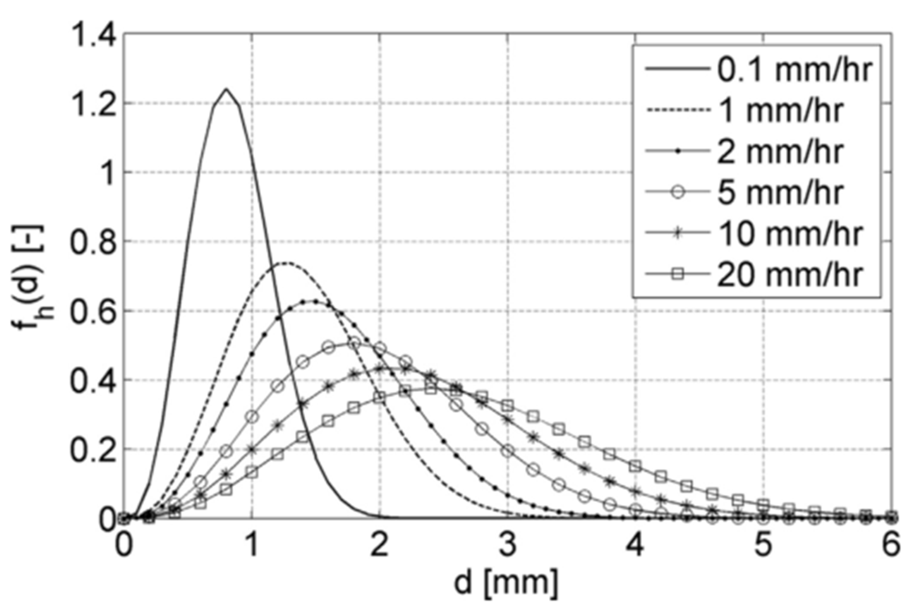
After determining the trajectory of the raindrops of different diameters, the capture ratio of raindrops of different diameters on the wind-turbine surface can be obtained. Then, the entire capture ratio of the wind-turbine surface can be calculated according to the horizontal distribution of raindrops with size (Figure 1).

Steps B and C require a continuous trial-and-correct process because the location of the raindrop injection cannot be easily determined. If the location of the raindrop injection is improperly selected, then the entire wind-turbine surface cannot be completely covered by rain. In such a trial-and-correct process, the three quantities of raindrop diameter, wind speed and wind direction need to be tried in different combinations [8]. In addition, the LPT model requires a very small grid size, and the number of grids generally exceeds 50 million.

Pan [9] used the LPT model to simulate the WAR phenomenon of the building facade and obtained the influence of wind direction on WAR distribution on the building’s windward side. Han Han [10] and Chen Yusheng [11] used a fluent-based LPT model to simulate the WAR phenomenon for different types of simple buildings, showing the influencing factors of the WAR phenomenon. By comparing with the experiment, the error of the specific rain-capture rate on the surface of the object in their numerical simulation is large due to the limitation of the LPT model. Eleni C. and Douvi [12] simulated the lift and drag coefficients of NACA0012 airfoil at different angles of attack under dry and wet conditions by self-programming, and finally obtained the effect of rain on airfoil performance. Shitang Ke and Wenlin Yu [13] also used the Lagrange particle-tracking method to analyze the influence of wind and rain on the aerodynamic performance of wind turbines at different yaw angles. In the research of [9,10,11,12,13], the number of computing grids exceeded 13 million, and the higher computational expenditure was required in these studies.

At present, the numerical simulation of rain conditions basically adopts the LPT model at home and abroad. Due to the higher computational expenditure of the LPT model, the development of this research area is seriously hindered. In order to overcome the limitations of the LPT model, in recent years, a new numerical method of simulating rain conditions has begun to develop, which is the Euler multiphase-model method. In 2010, the combination of the Eulerian multiphase model and RANS modeling has achieved remarkable results in the WAR calculation of isolated buildings. Huang and Li [14] used the Eulerian multiphase model with RANS, and the results showed that the model can give accurate results for the simulation of isolated buildings under WAR conditions. Briggen [15] predicted the wettability on the surface of a tower under WAR conditions based on the EM model and the LPT model, and both results were compared with the measurement results. The results showed that, when compared with the LPT model, the time cost of the EM model to simulate the WAR was reduced significantly due to the reduction in the number of grids, and both models were accurate. In conclusion, compared with the LPT model, the EM model has lower computational complexity, simpler quantification of the effect of raindrop turbulent diffusion, faster calculation, and higher computational efficiency. Therefore, this paper uses the EM model to realize the simulation of WAR, which makes up for the deficiencies of the LPT model and promotes the development of the field of numerical simulation of wind and rain.

In order to promote the development of the field of numerical simulation of rain conditions, considering that the EM model has more advantages than the LPT model in simulating the WAR phenomenon, the following studies are done based on the EM model. Compared with all previous related studies, this paper adopts a new numerical theory and model, which saves a lot of computing resources and time. In addition, under the premise of accurate results, it can simulate rainfall with common rainfall intensity, making up for the inadequacy of LPT model. In this paper, the load responses of wind turbines at different phase angles (0°, 30° and 60°) and to different wind speeds and different rainfall intensities are simulated. Finally, an envelope diagram of the influence coefficient of rain-induced loads is obtained, which provides a quantitative reference standard for the calculation of the load effect of objects under wind and rain conditions.

2. Materials and Methods

2.1. Principle and Method of Numerical Calculation

2.1.1. Wind-Phase Numerical Simulation

At present, the main CFD method to simulate a wind field is to solve the N-S equation. Select the steady-state SIMPLE algorithm of OpenFoam to simulate the stable wind field around the wind turbines. There are two key points in the SIMPLE algorithm: (1) The Poisson pressure equation is derived from the momentum and continuity equations, and (2) the velocity-correction equation is derived to satisfy the continuity equation. The KOmegaSST turbulence model is used to simulate the incompressible turbulent wind. The KOmegaSST turbulence model considers the transfer of turbulent shear stress on the basis of the standard k-ω model, and also considers the low Reynolds number, compressibility and shear-flow propagation [16,17].

The control equation is as follows:

$$\frac{\partial u_j}{\partial x_j}=0$$

(1)

$$\frac{\partial {\rho }_a{u}_i}{\partial t}+\frac{\partial \left({\rho }_a{u}_i{u}_j\right)}{\delta x_j}=-\frac{\partial p}{\partial x_i}+\frac{\partial {\tau }_{ij}}{\delta x_j}$$

(2)

$$\frac{\partial {\rho }_{a}k}{\partial t}+\frac{\partial \left({\rho }_{a}k{u}_j\right)}{\partial x_j}=\frac{\partial }{\partial x_j}\left[\left(\mu +\frac{{\mu }_t}{{\sigma }_k}\right)\frac{\partial k}{\partial x_j}\right]+G_k-{\rho }_a\epsilon$$

(3)

$$\frac{\partial {\rho }_a\epsilon }{\partial t}+\frac{\partial \left({\rho }_a\epsilon u_j\right)}{\partial x_j}=\frac{\partial }{\partial x_j}\left[\left(\mu +\frac{{\mu }_t}{{\sigma }_{\epsilon }}\right)\frac{\partial \epsilon }{\partial x_j}\right]+C_{1\epsilon }\frac{\epsilon }{k}{G}_k-C_{2\epsilon }{\rho }_a\frac{{\epsilon }^2}{k}$$

(4)

$${\mu }_t=C_{\mu }{\rho }_a\frac{k^2}{\epsilon }$$

(5)

where ${\rho }_a$ represents the density of air, $p$ is the pressure of air, k is the turbulent kinetic energy, $\epsilon$ represents the turbulent diffusion rate, ${\tau }_{ij}$ represents the Reynolds stress, $\mu$ represents the air viscosity, μ_t represents the turbulent viscosity of air, $G_k$ represents the turbulent kinetic-energy gradient generated by the average velocity, $C_{\mu }=0.11$, $C_{2\epsilon }=1.92$, $C_{1\epsilon }=1.44\mathrm{and}{\sigma }_{\epsilon }=1.2$.

2.1.2. Rain-Phase Numerical Simulation

After the stable wind field is obtained by the SIMPLE algorithm, the rain phases are injected at the boundary of the computational domain. Under a certain rainfall intensity, different sizes of raindrops can be selected according to the best measurement [18] (Figure 1). Each size corresponds to each rain phase in the multiphase model. After the rain of different sizes is injected into the wind field, it moves under the single coupling effect of wind. The flow-control equation is as follows.

$$\frac{\delta {\rho }_w{\alpha }_k}{\delta t}+\frac{\delta \left({\rho }_w{\alpha }_k{u}_{\mathrm{kj}}\right)}{\delta x_j}=0$$

(6)

$$\frac{\delta {\rho }_w{\alpha }_k{u}_{\mathrm{ki}}}{\delta t}+\frac{\delta \left({\rho }_w{\alpha }_k{u}_{\mathrm{k}\mathrm{i}}{u}_{\mathrm{kj}}\right)}{\delta x_j}={\rho }_w{\alpha }_{k}g+{\rho }_w{a}_k\frac{3\mu }{{\rho }_w{d}^2}\frac{C_d{\mathrm{Re}}_R}{4}\left(u_i-u_{\mathrm{ki}}\right)$$

(7)

where d is the raindrop diameter, $a_k$ is the volume fraction of the k-phase rain, $u_{\mathrm{k}\mathrm{i}}$ is the velocity component of the k-phase rain, $u_i$ is the velocity component of the wind, ${\rho }_w$ is raindrop density, g is gravitational acceleration and $C_d$ is the drag coefficient. For the relative Reynolds number ${\mathrm{Re}}_R$, the calculation formula is as follows:

$${\mathrm{Re}}_R=\frac{{\rho }_{a}d}{\mu }\left|\overrightarrow{u}-{\overrightarrow{u}}_k\right|$$

(8)

where $\overrightarrow{u}$ is the wind-phase velocity and ${\overrightarrow{u}}_k$ is the rain-phase velocity.

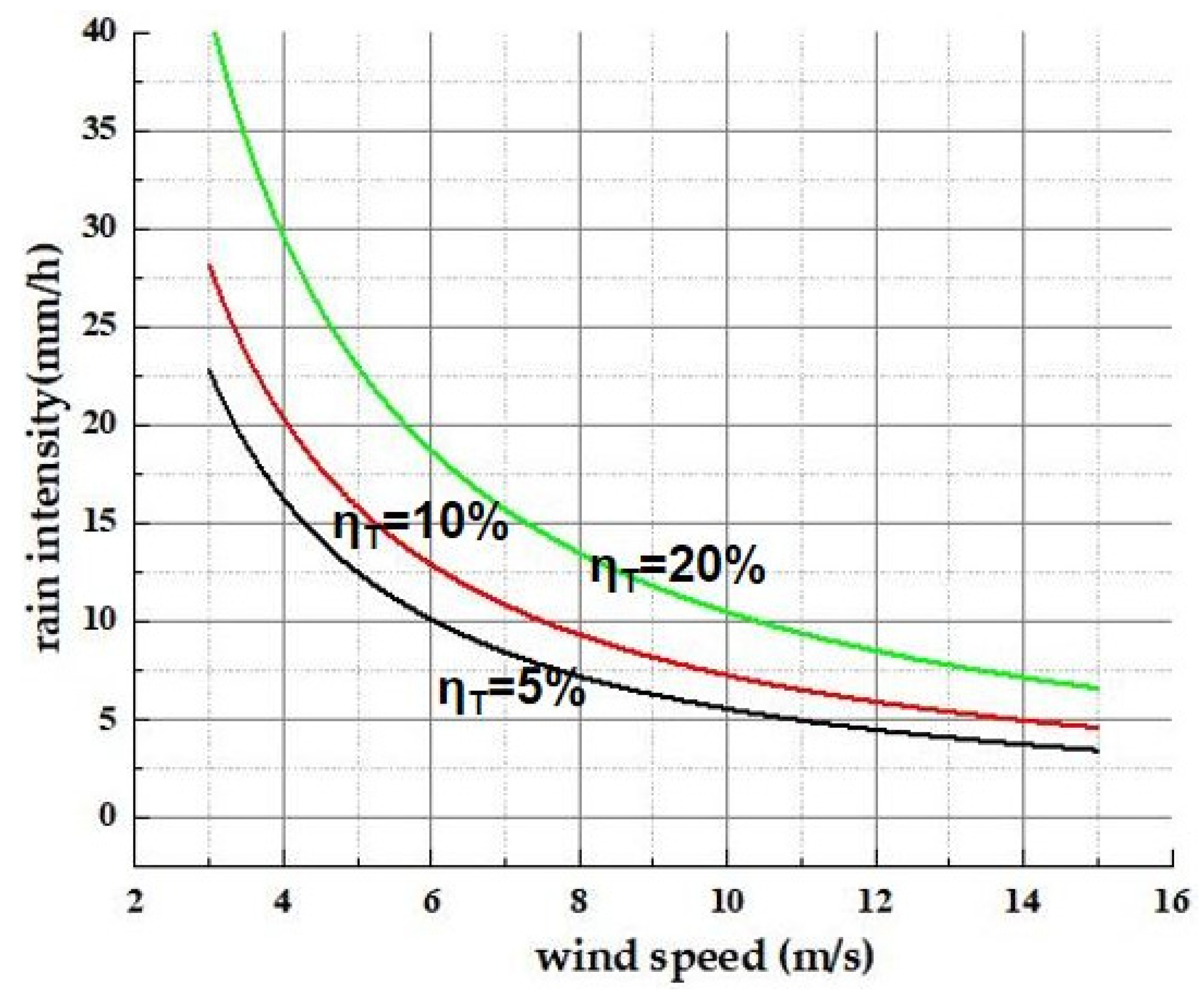
2.1.3. Parameters of WAR

The most intuitive parameter for the intensity of the WAR on the wind turbines is the capture ratio defined by Blocken, B. and Carmeliet, J. in 2004 [2]. The global capture ratio of a surface is directly related to the specific capture ratio of each rain phase, and the calculation formulas are as follows:

$${\eta }_d\left(k\right)=\frac{R_{\mathrm{WAR}}\left(k\right)}{R_h\left(k\right)}=\frac{{\alpha }_k\left|V_n\left(k\right)\right|}{R_h{f}_h\left(k\right)}$$

(9)

$$\eta ={\int }_d{f}_h(R_h,d){\eta }_d\mathrm{d}d$$

(10)

where $d$ is the radius of the k-th phase of rain, $R_{wdr}\left(k\right)$ is the intensity of wind action,$R_h$ is the rainfall intensity of rain passing through the horizontal plane, ${\alpha }_k$ is the phase fraction of the k-th phase of rain and $V_n\left(k\right)$ is the velocity vector of the k-th phase of rain. $f_h\left(R_h,d\right)$ is the probability-distribution value of the size of the rain phase on the horizontal plane. It is necessary to refer to Figure 1, which is the data map of the size distribution of raindrops passing through the horizontal plane calculated by the best measurement [18]. $f_h\left(k\right)$ is the probability-distribution value of the k-th rain phase. ${\eta }_d$ is the capture ratio of rain with diameter d.

The process of rain impacting on the surface of wind turbines agrees with the momentum theorem. Based on the raindrop-collision theory elaborated by Chen [19], if ignoring the evaporation, splash and rupture of raindrops on the surface of wind turbines, then the interaction between rain and the structure follows Newton’s second law. The collision force of rain on the tiny area of the wind-turbine surface is ($V_s$ is the final rain speed):

$$F=\rho \eta R_h{\Delta }_s{V}_s$$

(11)

The rain load on the whole surface of the wind turbine is calculated by integrating the whole surface of the wind turbine.

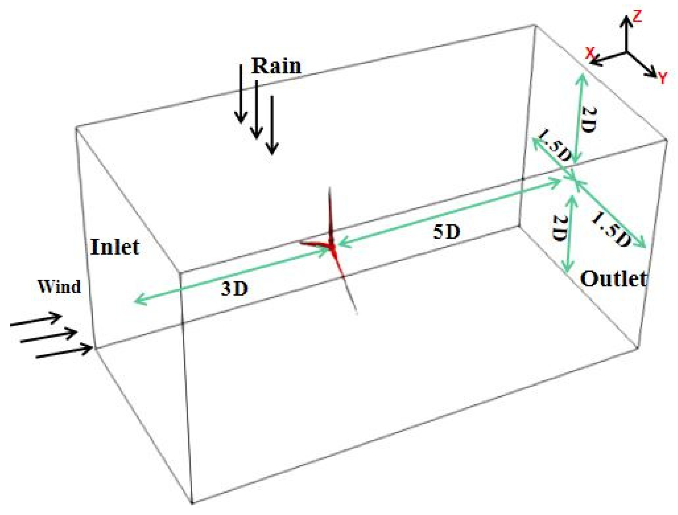
2.1.4. Numerical-Simulation Settings

Figure 2 shows the optimal calculation-domain size determined after verification. The front and back of the calculation domain are symmetrical. The left and right are the inlet and outlet, and the top is the surface where the rain phases are injected. Figure 3 shows the local grid. The number of grids in this study is 840,000, whereas under the same conditions, the number of grids in the paper of Shitang Ke and Wenlin Yu [13] exceeded 14 million, proving that this EM model can save much time.

In this paper, the method of realizing the WAR phenomenon involves injecting the rain phase into the stable wind field. It is different from the LPT model, for which it is necessary to constantly try different wind speeds, wind-speed directions, and raindrop-injection positions. The whole process of the EM model is simple and time saving.

2.2. Numerical Comparison and Analysis

In this section, the numerical results of Shitang Ke and Wenlin Yu [13] are compared in order to verify the accuracy of the self-compiled solver in the simulation of WAR. Shitang Ke and Wenlin Yu used the Lagrange particle-tracking model (LPT) to calculate the aerodynamic wind and rain loads of NUAA 5 MW wind turbines. The rainfall intensity was 64 mm/h, the wind speed was 25 m/s and the phase angle of the wind turbines was 0°. Although the maximum rainfall intensity in Figure 1 is 20 mm/h, the distribution of 64 mm/h rainfall intensity can be deduced from the law in Figure 1. Figure 4 shows the average horizontal velocity of raindrops of different sizes before they finally hit the wind-turbine surface.

It can be seen from the data that with the increase in raindrop diameter, the average velocity of raindrops also rises. When the raindrop size is small, the difference between the data in this study and the comparative data is approximately 13%, but both sets of data are consistent in the comparison of medium-sized and large-sized raindrops. Under the rainfall intensity of 64 mm/h, the sizes of raindrops are mainly above 3 mm, and few are below 1 mm. Moreover, the rain-induced loads were mainly reduced by the rain phases with large sizes, so the error of 13% can be ignored.

When the wind-turbine phase angle is 0°, the bottom blade is named blade A, and the remaining two blades are named blade B and blade C along the clockwise direction. Figure 5a shows the distribution of rain-induced pressure of the three blades along the length direction. Figure 5b shows the distribution of the rain-induced-pressure coefficient of the three blades along the length direction. The difference between the calculation results of this study and the comparative data is within 10%.

3. Results and Discussion

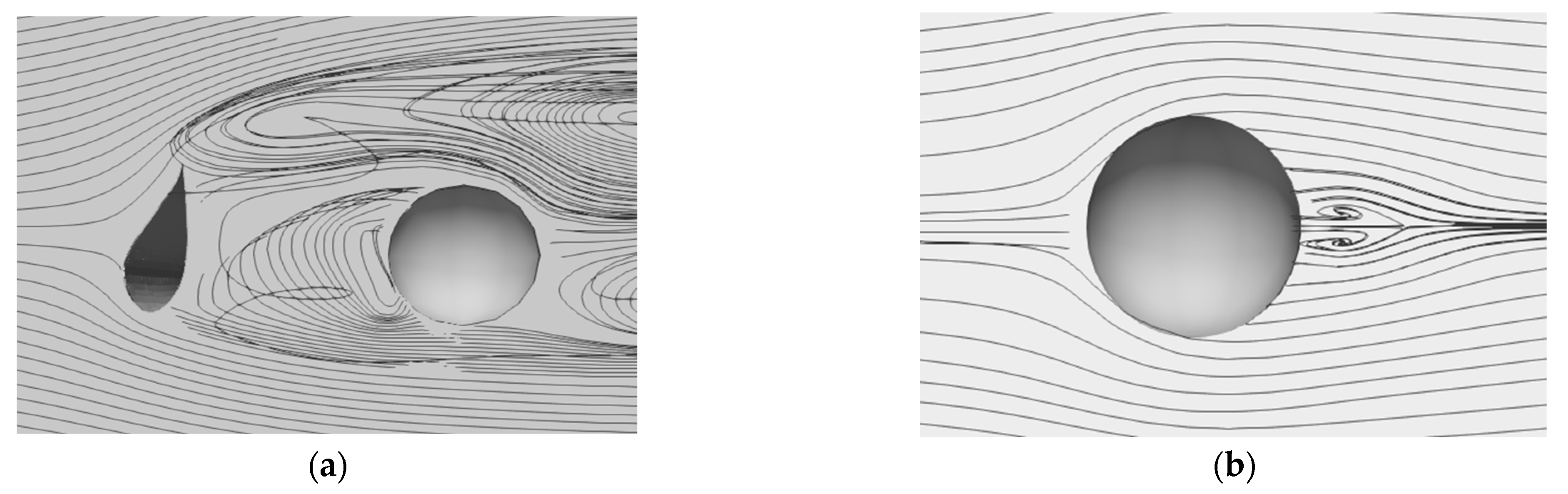
3.1. Aerodynamic Analysis of Pure Wind Field

As shown in Figure 6, three representative phases, α = 0°, 30° and 60°, of the wind turbine are selected, and the naming rules of the blades at different phases are also shown.

Generally, for the tower, the area of the blade-radius erosion cover is the disturbance area, and the other parts are the non-disturbance area [20]. The section at 20 m is taken as the typical section of the disturbance area, and the section at 80 m is the typical section of the non-disturbance area. Figure 7 shows the wind-pressure contour map of the typical section under the wind speed of 10 m/s at different phase angles, and the value on the contour is the relative value after dimensionless treatment. Figure 8 analyzes the circumferential-pressure-coefficient distribution of two typical sections of the tower under different conditions. Through analysis, it can be found that when the wind-turbine phase angle is 0°, the blade completely blocks the tower, resulting in the negative pressure of the typical section of the tower. In addition, at other phase angles, the position of the maximum positive pressure on the tower is 270°, and the position of the maximum negative pressure is 0°. The farther the blade is away from the tower, the less the tower force is affected by the blades.

Figure 9 is the wind-field streamline diagram of the typical section of the disturbed area and the non-disturbance area. It can clearly find the obvious flow phenomenon when the wind field flows through the building, and the vortex is formed behind the object.

The wind-turbine blades with different phase angles are named as shown in Figure 6. Figure 10 shows the wind-induced loads along the height direction of the tower and the radial direction of the blades. The horizontal axis represents the maximum wind pressure on the windward side of the blades or tower. Blades A and C at α = 60° and blades A and B at α = 0° are approximately symmetrical structures, and the pressure distributions have similar regularity.

When the phase angle is 0°, due to the full occlusion of the blade, there is a sudden change in the force at 30 m for the tower, and the pressure changes from positive pressure to large negative pressure.

3.2. Analysis under the Simultaneous Action of Wind and Rain

After the aerodynamic analysis of the wind turbine in the pure wind field, the numerical simulation of the still wind turbine under WAR conditions is carried out, and the results are compared with those in the previous section. The rainfall intensity is 5 mm/h.

The rain field is constructed by injecting rain phases with different raindrop sizes at the top and inlet of the stable-wind-field domain. The boundary conditions of the rain phase require α and U parameters. After the rain phases are injected into the wind field, the one-way wind acts on the rain phases, and the control equation of the rain phases under the one-way wind is solved. Then, the control parameters α and U of the rain phases are obtained, and then the rain distribution on the wind-turbine surface can be obtained. Finally, according to the collision theory, the rain load is calculated.

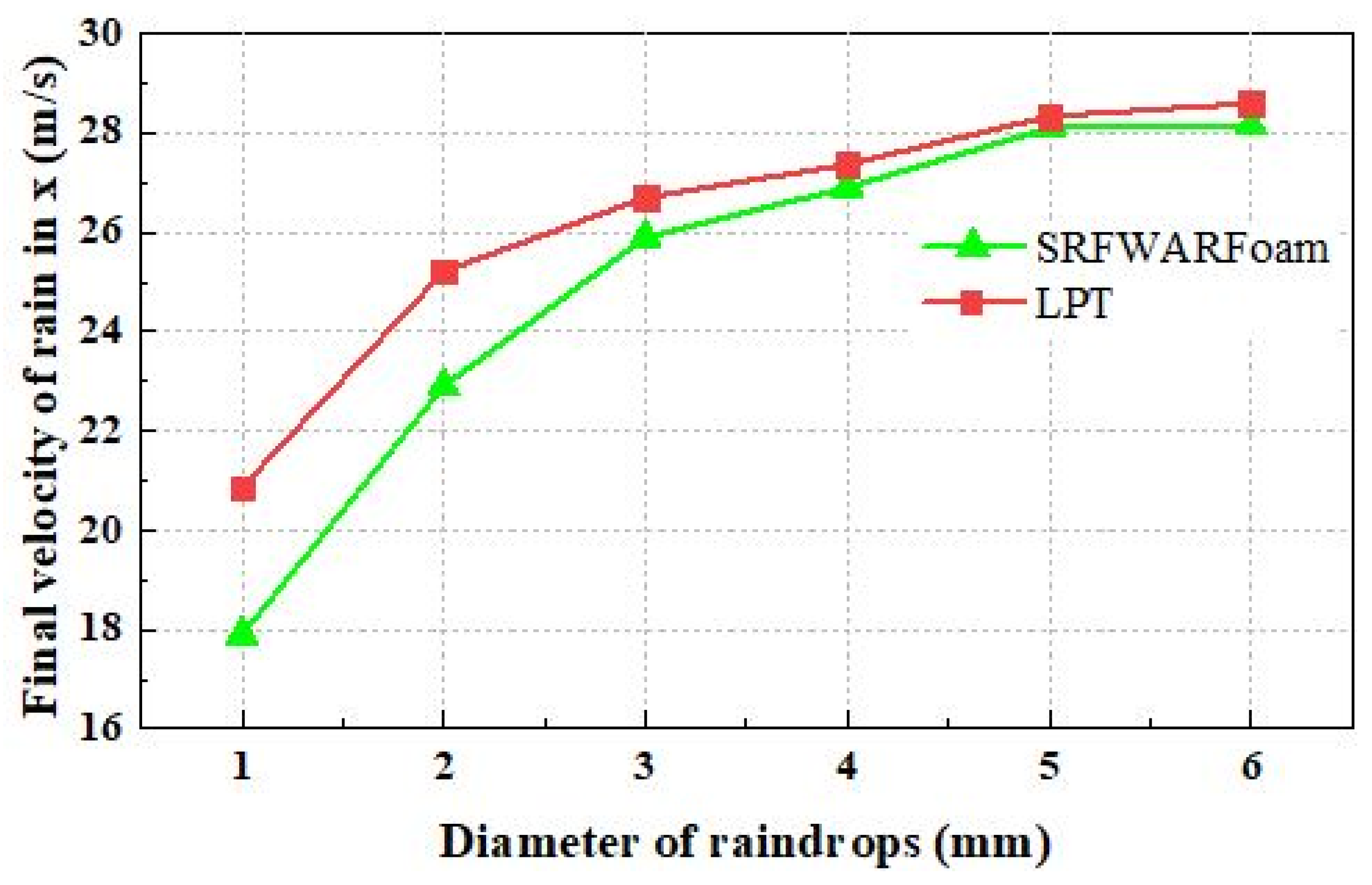
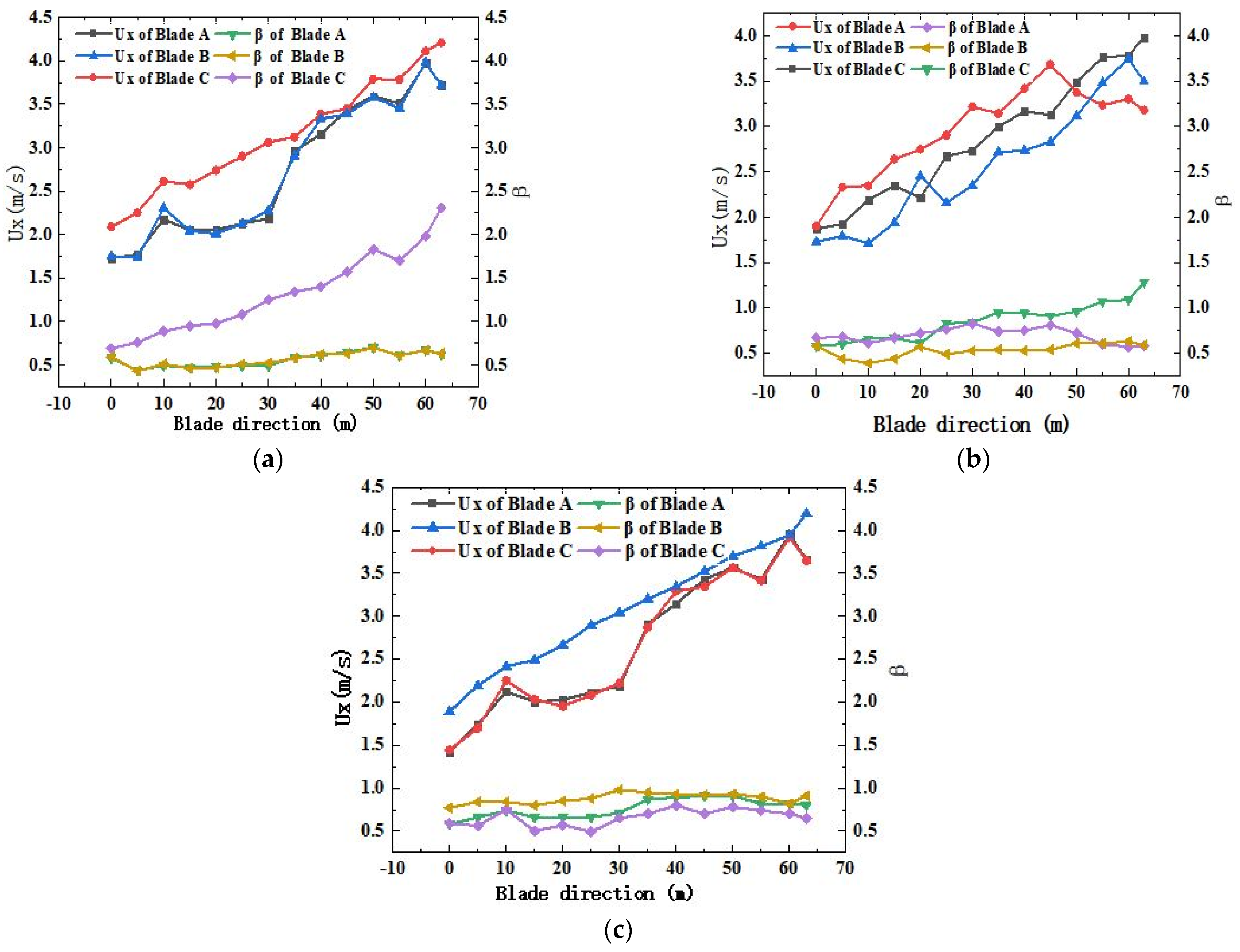
3.2.1. The Final Velocity of Rain along Blade Direction

After the wind-and-rain coupling in the calculation domain, there is a final velocity before the rain phases collide with the surface of the wind turbine, which directly affects the size and direction of the rain-induced loads.

The initial raindrop velocity should be U_Z along the Z direction. However, after the rain phases enter the wind field, it will have a horizontal velocity U_X after the effect of the wind. A new parameter β is defined as the value of U_X/U_Z. Taking the weighted average of the final velocity of all sizes of the rain phases, Figure 11 shows the final rain velocity along the radial variation of the blade at different phase angles. The wind speed is 8 m/s and rain intensity is 5 mm/h.

As shown in Figure 11a, since blades A and B are approximately symmetrical structures, the distribution of the rain’s final velocity is basically consistent. When α = 0°, blade C is at the lowest position, and the rain’s final velocity U_Z is relatively small, resulting in parameter β being greater than 1. In Figure 11c, blades A and C are approximately symmetrical structures.

The rain’s final velocity U_X increases gradually along the radial direction because the closer the rain is to the tip of blades, the more obvious the phenomenon of windblown rain becomes. For the rain’s final velocity U_Z, because the rain is mainly injected at the top, the velocity component also shows a decreasing trend from bottom to top, and the velocity at the root of each blade is basically consistent.

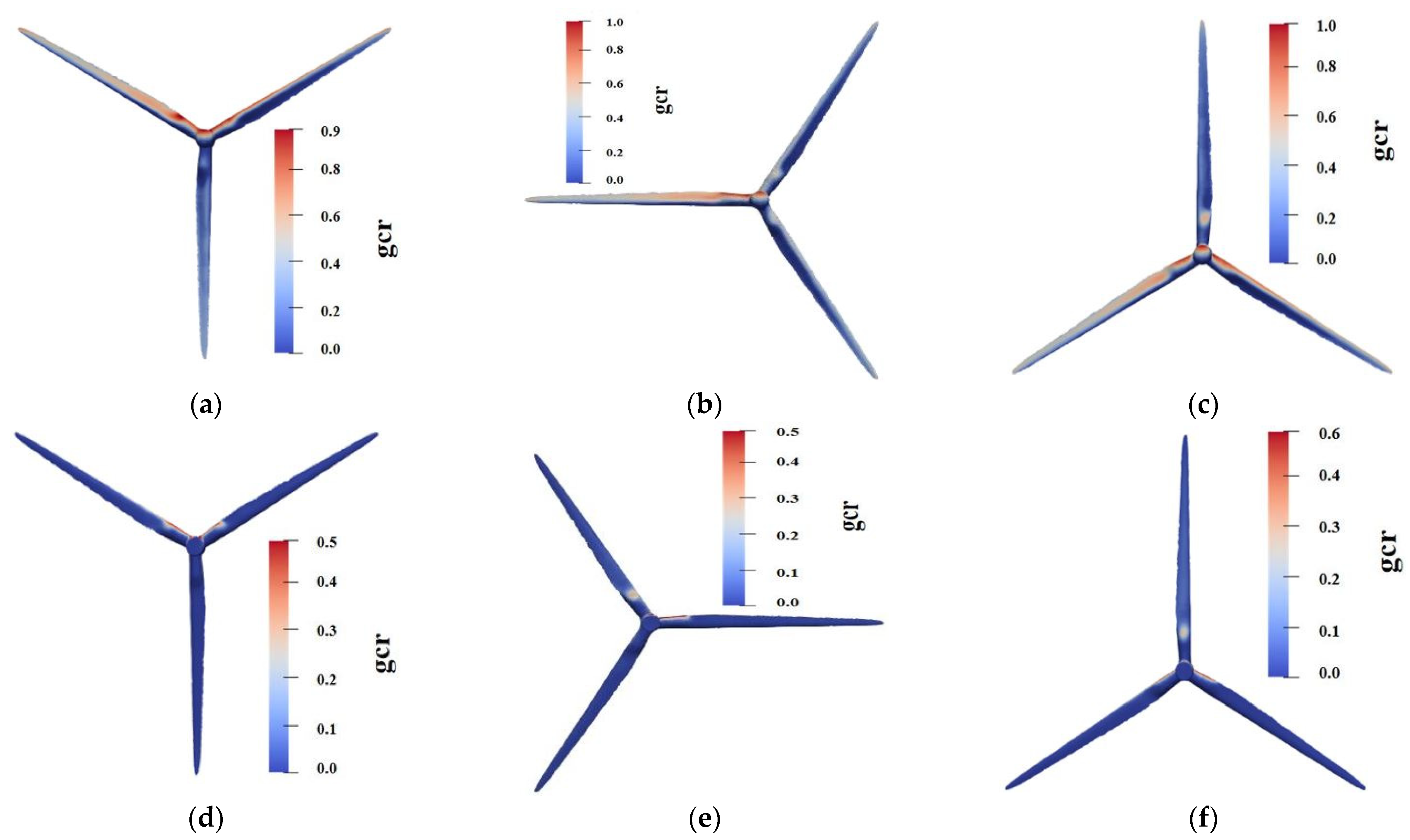
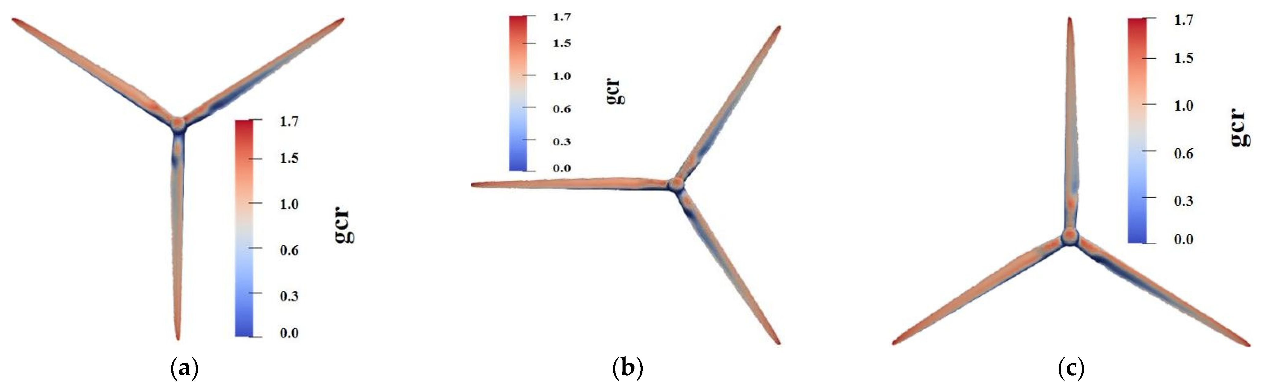
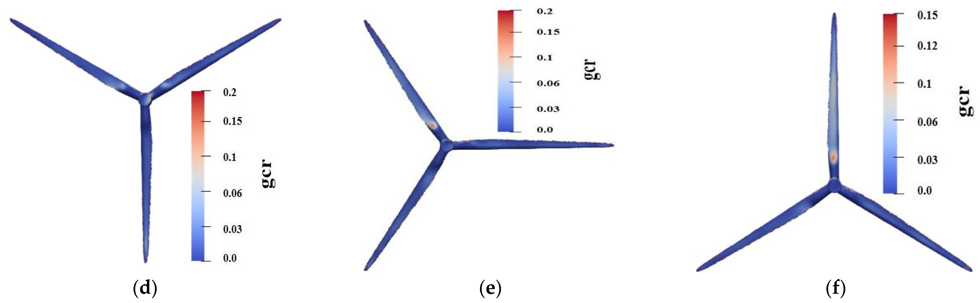
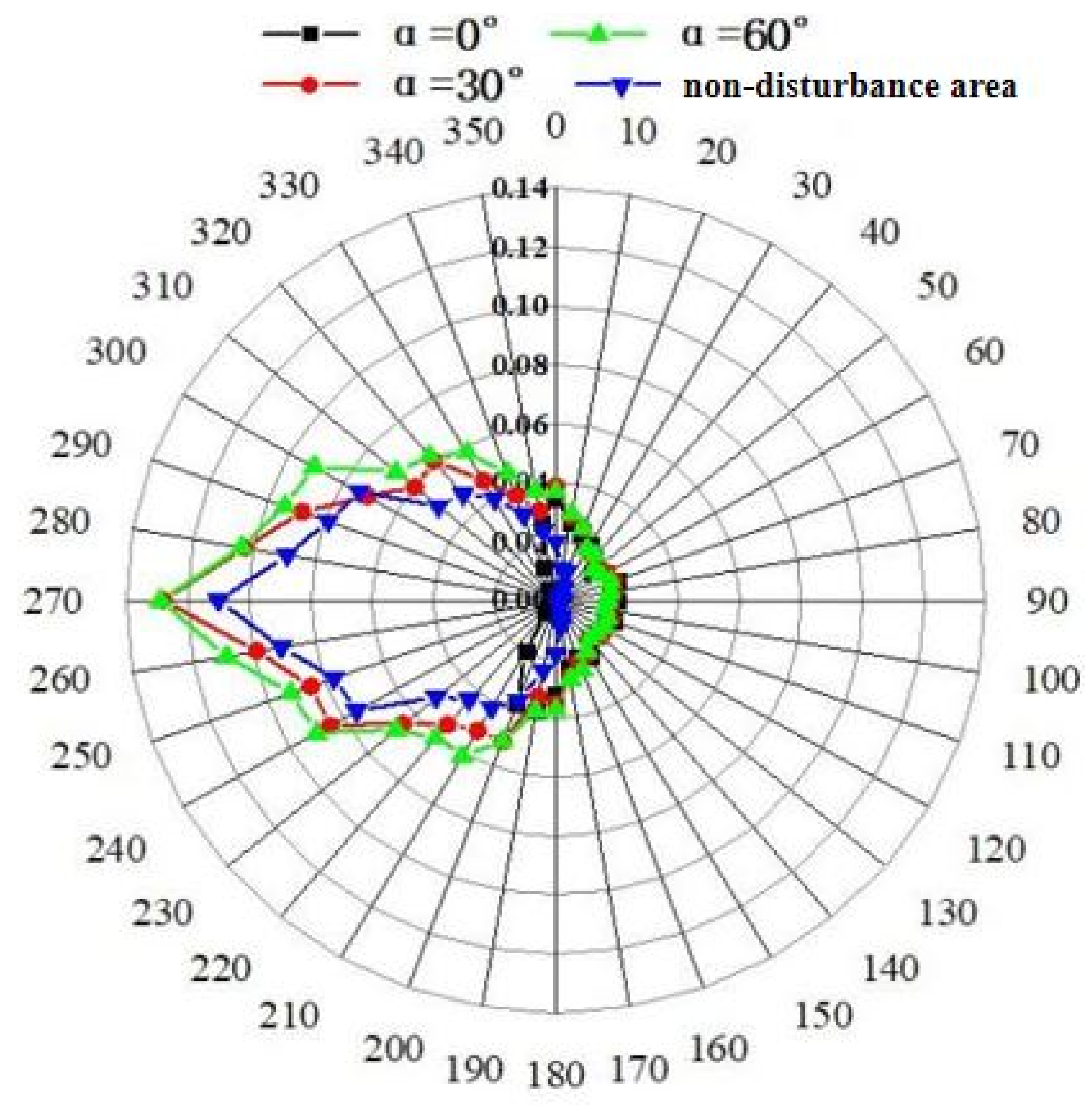
3.2.2. The Capture Ratio of Rain

After the effect of wind, the capture ratio is a direct indicator to describe the distribution of rain on the wind-turbine surface. The rain-capture ratio is defined as the ratio of the rainfall intensity on the wind-turbine surface to the horizontal rainfall intensity. The specific calculation method is shown in Chapter 1. Figure 12 and Figure 13 show the distribution of the rain-capture ratio at different wind speeds and different phase angles.

When the wind speed is small, the rain phases are hardly affected by the horizontal force of the wind, and the rain nearly keeps its original motion state and path. The rain on the windward side of the wind turbine is less, and the rain is mainly concentrated on the shoulder of the wind turbine and the prominent shaft. There is also rain on the back of the wind turbine.

When the wind speed increases to 10 m/s, the rain on the windward side of the wind turbine is doubled and evenly distributes on the windward side because of the strong horizontal wind loads. At this high wind speed, the rain on the back of the wind turbine is much less, and the maximum capture ratio is about 0.1.

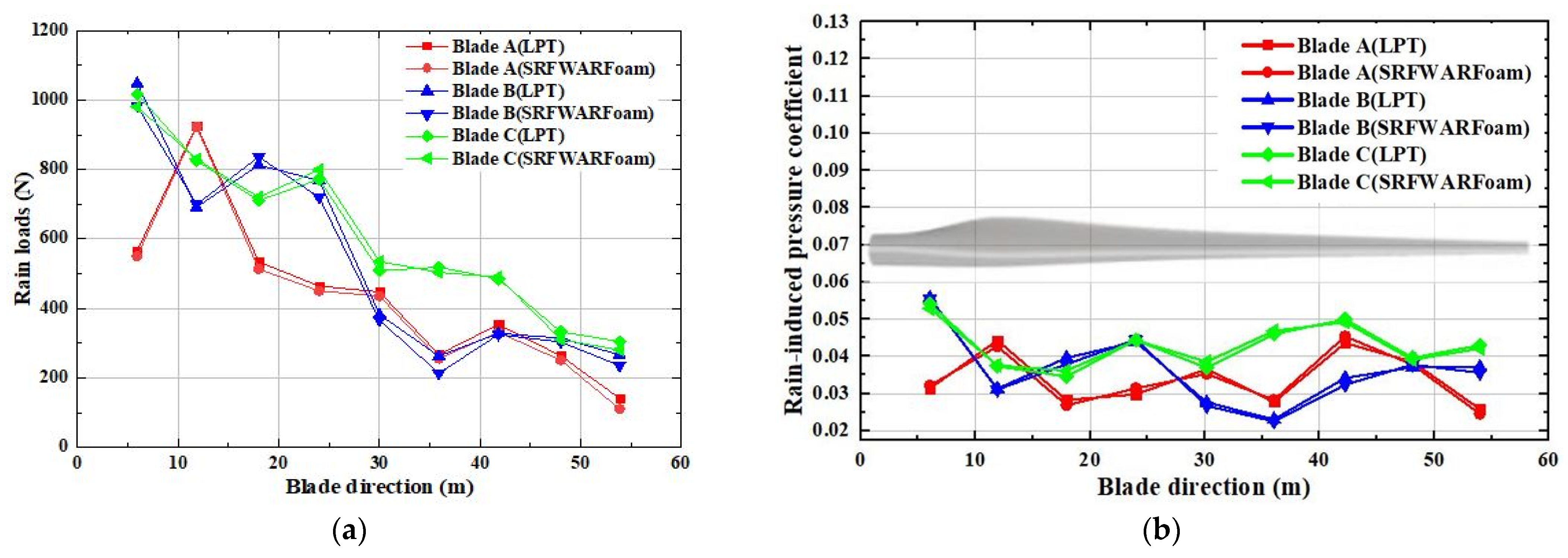
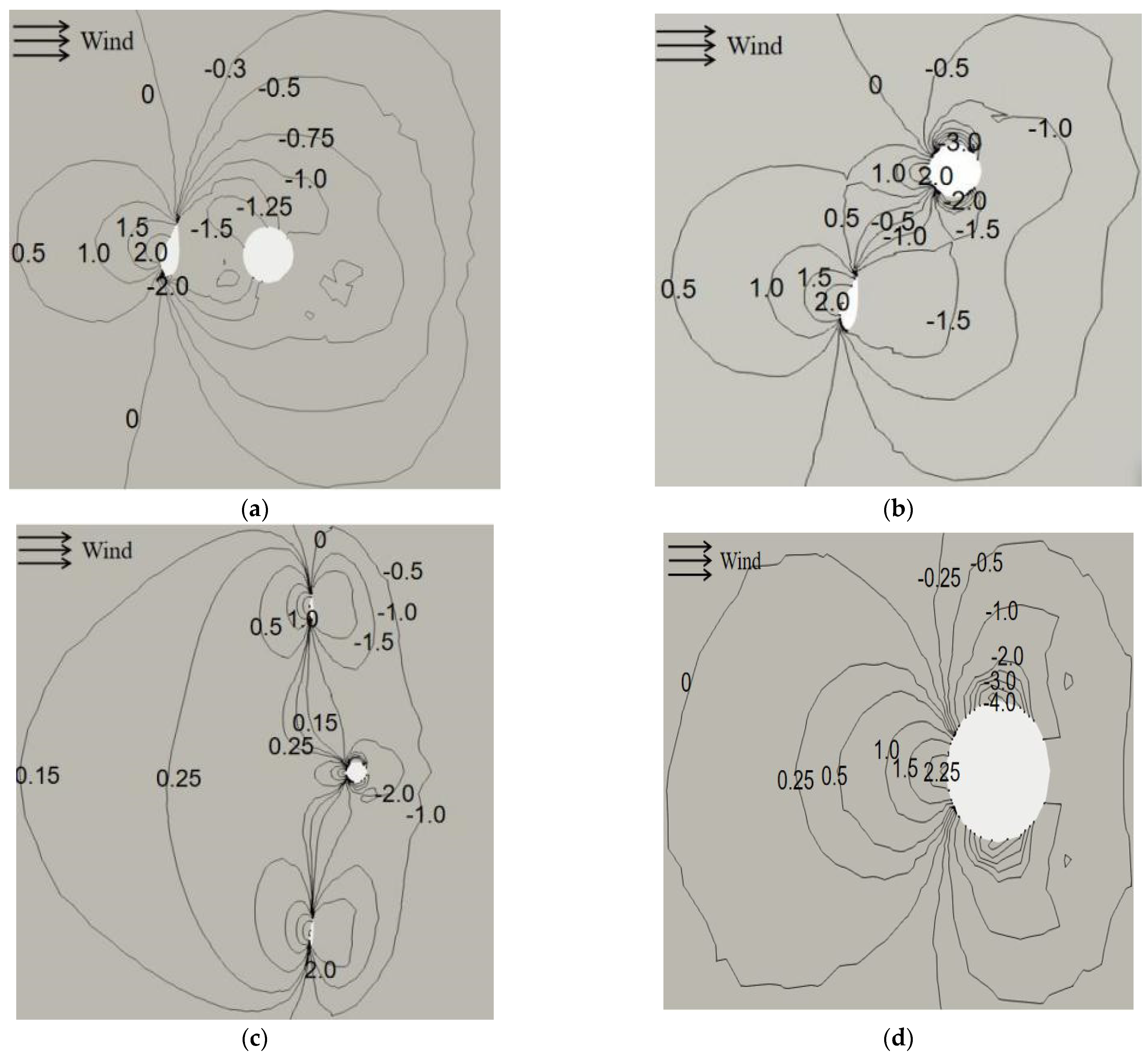
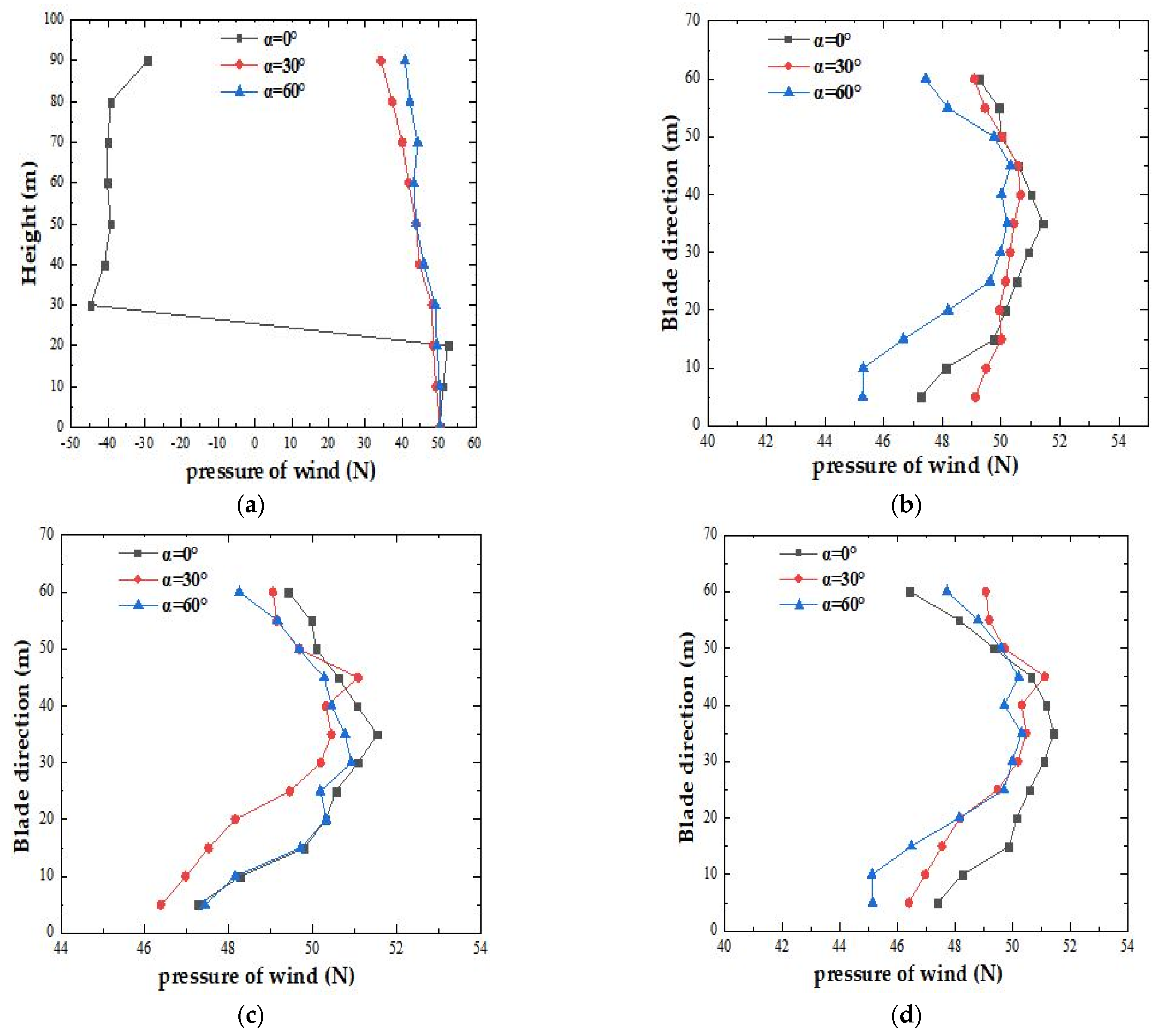
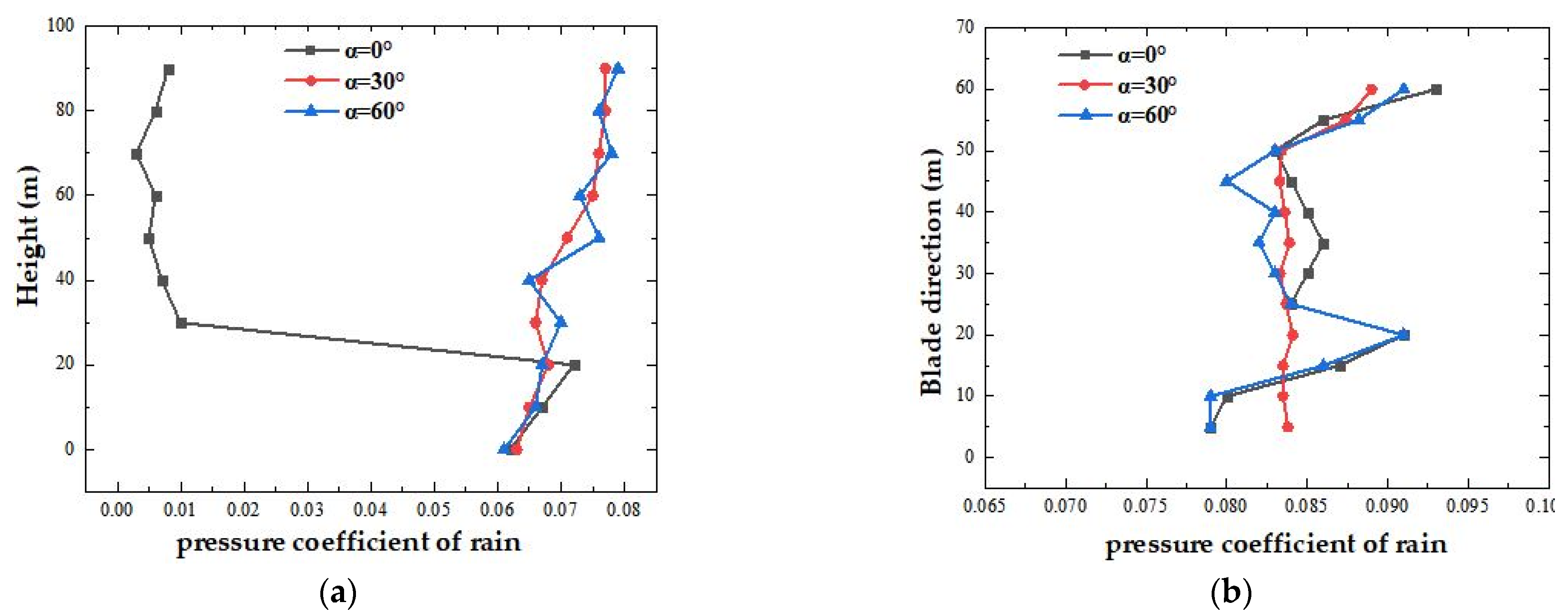
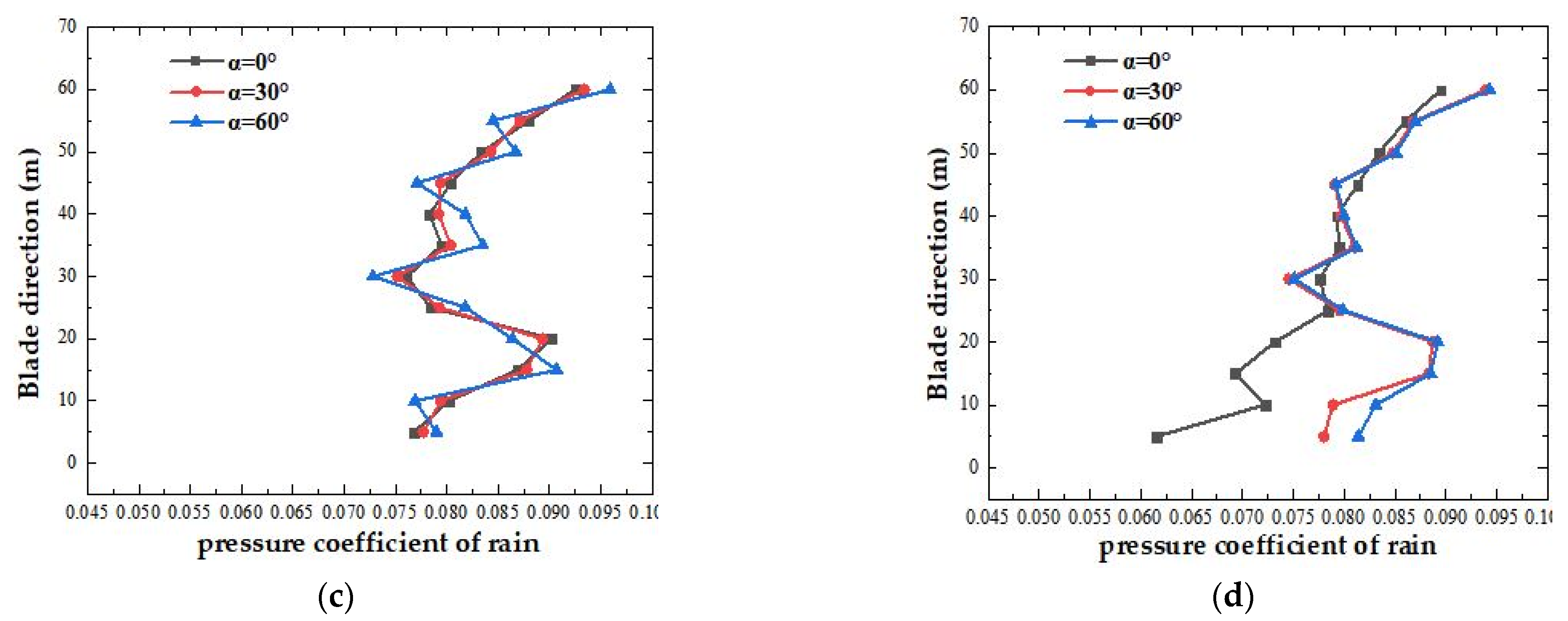
3.2.3. Distribution of Rain Pressure on Tower and Blade

According to the previous section, two typical sections of the disturbance area and the non-disturbance area are selected. Figure 14 analyzes the circumferential distribution of the rain-induced-pressure coefficient on the typical section at a wind speed of 10 m/s. For the convenience of drawing, the rain-induced-pressure coefficient is amplified by the amplification factor (k = 5). The rain-induced-pressure coefficient ${\mathrm{C}}_{\mathrm{P}}$ is calculated using Formula (12). P_R is the rain pressure and P_Z0 is the wind pressure at the reference height.

$${\mathrm{C}}_{\mathrm{P}}=\frac{{\mathrm{P}}_{\mathrm{R}}}{{\mathrm{P}}_{\mathrm{Z}0}}$$

(12)

The physical position of the blade is higher than that in the non-disturbance area, so the rainfall-induced pressure is greater in the typical section of disturbance area. When α = 0°, the blade completely blocks the tower, and the pressure coefficient is minimized. The rain-induced-pressure coefficient of the leeward surface (0–180°) of the two typical sections of the tower is very small, because it is only affected by a small amount of free-falling raindrops.

Figure 15 analyzes the distribution of rain-induced-pressure coefficients (amplified by the amplification factor k = 5) along the height direction of the tower and the radial direction of blades A, B and C at different phase angles and at a wind speed of 10 m/s.

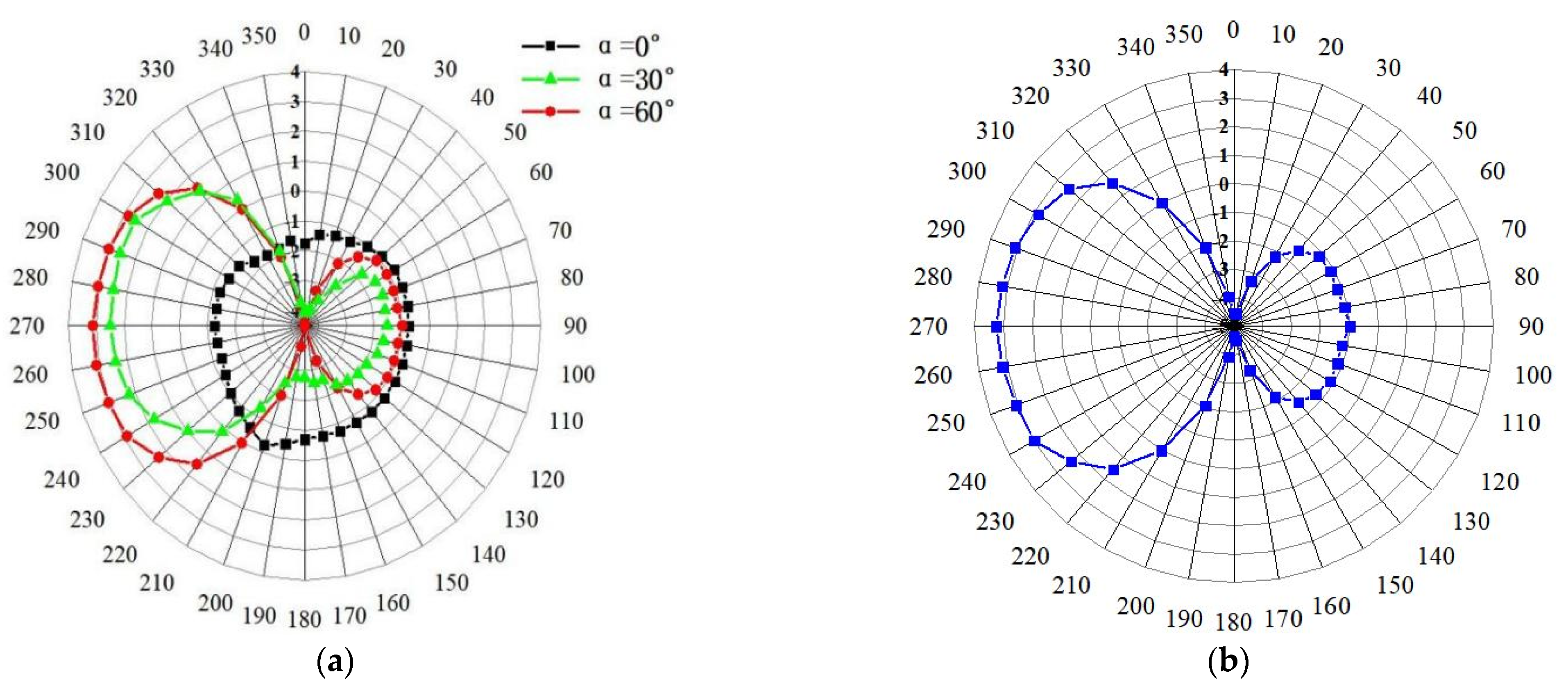
3.3. The Fitting Curve of Rain-Induced Influence Coefficient

In order to find the quantitative regularity of the rain-induced loads on the wind turbine related the wind speed and rainfall intensity, this study needs more working conditions based on the existing conclusions. A new parameter η_T is defined. The calculation formula of this parameter is as follows:

$${\mathsf{\eta }}_{\mathrm{T}}=\frac{T_R}{T_W}$$

(13)

where $T_R$ is the rain-induced thrust of the wind turbine and $T_W$ is the wind thrust of the wind turbine.

The parameter η_T is only related to the wind speed and the rain intensity and is not affected by the different phase angles of the wind turbine. Taking η_T = 5%, η_T = 10%, and η_T = 20% as the characteristic lines, the envelope lines in Figure 16 are fitted to a greater number of numerical results, which can be a reference for future researchers. Take characteristic line η_T = 5%, for example. When the rainfall intensity is 10 mm/h, the wind speed exceeds 6 m/s and η_T exceeds 5%.

4. Conclusions

This paper uses the WARFoam solver based on the EM model to compare and analyze the load response of wind turbines under WAR conditions. By comparing its results with the rain-induced loads simulated by the Lagrange particle-tracking model, it is verified that the research method in this study is accurate, time saving and comprehensive in simulating the rain distribution and calculating the rain-induced loads. The EM model has lower computational complexity and higher computational efficiency due to the reduction in the number of grids compared to the LPT model. At the same time, on the basis of overcoming the shortcomings of the LPT model, this paper accurately models the WAR phenomenon and the wind-and-rain-load characteristics of wind turbines under different conditions. Therefore, the new method of the EM model used in this paper can compensate for the insufficiency of the LPT method, thereby saving a lot of computing resources and time, and it can successfully numerically simulate the load response to the common rainfall intensity of wind turbines.

The motion trajectory of raindrops is jointly affected by gravity and wind force. When the wind speed is small, the rain phase moves almost parallel to the surface of the wind turbine. The greater the wind speed is, the greater the horizontal force on the rain phase is, and the greater the horizontal component of the rain-phase velocity is. Greater rainfall intensity requires a greater wind speed in order for the rain phase to have an influential horizontal velocity.

Through the analysis of the final velocity of the rain before it hits the wind turbine, it is found that the windblown-rain phenomenon is more likely to affect the position near the tip of the blade, while the rain phase alone mainly affect the position near the blade root because the blade root is close to the rotating shaft, and the rotating shaft has sufficient contact with the rain falling vertically. Rain-induced loads act more on the blade tip and root. For the tower, the closer the blade is to the tower, the weaker the rain-induced loads are.

This study fitted the envelope diagram of the rain-induced-impaction coefficient to many calculation data and selected three representative characteristic lines, which can provide quantitative reference standards for future researchers.

Finally, the current research still has some shortcomings. Firstly, this study only considered the one-way coupling of raindrops with the wind flow, not wind–rain two-way coupling. Secondly, when calculating the load of the interaction between the raindrop and the structure, the splash of the raindrops and the formation of water film are ignored. Based on the above limitations, the method proposed in this paper cannot be applied to a dynamic wind turbine and there is much to be improved in terms of engineering applications; therefore, the numerical simulation will be improved in future research, and more studies will be performed on dynamic wind turbines under WAR conditions.

References

1. Blocken, B.; Carmeliet, J. Blocken B, Carmeliet J. Overview of three state-of-the-art wind-driven rain assessment models and comparison based on model theory. Build Environ. 2010, 45, 691–703. [Google Scholar] [CrossRef]
2. Blocken, B.; Carmeliet, J. A review of wind-driven rain research in building science. J. Wind Eng. Ind. Aerodyn. 2004, 92, 1079–1130. [Google Scholar] [CrossRef]
3. Blocken, B.; Carmeliet, J. High-resolution wind-driven rain measurements on a low-rise building-Experimental data for model development and model validation. J. Wind Eng. Ind. Aerodyn. 2005, 93, 905–928. [Google Scholar] [CrossRef]
4. Kubilay, A. Numerical Simulations and Field Experiments of Wetting of Building Facades Due to Wind-driven Rain in Urban Areas. Ph.D. Thesis, ETH Zurich, Zurich, Switzerland, 2014. [Google Scholar]
5. Nan-You, L.; Basu, S.; Manuel, L. On wind turbine loads during the evening transition period. Wind. Energy 2019, 22, 1288–1309. [Google Scholar]
6. Nandi, T.N.; Herrig, A.; Brasseur, J.G. Non-steady wind turbine response to daytime atmospheric turbulence. Phil. Trans. R. Soc. A 2017, 375, 20160103. [Google Scholar] [CrossRef] [PubMed] [Green Version]
7. Churchfield, M.J.; Lee, S.; Michalakes, J.; Moriarty, P.J. A numerical study of the effects of atmospheric and wake turbulence on wind turbine dynamics. J. Turbul. 2012, 13, N14. [Google Scholar] [CrossRef]
8. Blocken, B.; Carmeliet, J. Spatial and temporal distribution of driving rain on a low-rise building. Wind Struct. 2002, 5, 441–462. [Google Scholar] [CrossRef]
9. Pan, Z. Numerical Investigation about the Effects of the Wind Direction on WDR Distribution on Windward Building(s) Facades; Hefei University of Technology: Hefei, China, 2014. [Google Scholar]
10. Han, H. Research on Distribution Characteristics of Wind-Driven Rain on Building Envelopes; Hefei University of Technology: Hefei, China, 2013. [Google Scholar]
11. Chen, Y. Numerical Simulation Study on Aerodynamic Effect on Wind-Driven Rain on Building Facades; Hefei University of Technology: Hefei, China, 2017. [Google Scholar]
12. Eleni, C.D.; Margaris, D.P. Simulation of Heavy Rain Flow over a NACA0012 Airfoil. In Proceedings of the 4th International Conference on Experiments/Process/System Modeling/Simulation/Optimization (IC-EpsMsO), Athens, Greece, 6–9 July 2011. [Google Scholar]
13. Shitang, K.; Wenlin, Y. Aerodynamic performance and wind-induced effect of large-scale wind turbine system under yaw and wind and rain combination action. Renew. Energy 2019, 136, 235–253. [Google Scholar]
14. Huang, S.H.; Li, Q.S. Numerical simulations of wind-driven rain on building envelopes based on Eulerian multiphase model. J. Wind Eng. Ind. Aerodyn. 2010, 98, 843–857. [Google Scholar] [CrossRef]
15. Briggen, P.M.; Blocken, B.; Schellen, H.L. Wind-driven rain on the facade of a monumental tower: Numerical simulation, full-scale validation and sensitivity analysis. Build. Environ. 2009, 44, 1675–1690. [Google Scholar] [CrossRef]
16. Chen, Z.; Wang, X.; Guo, Y.; Kang, S. Numerical analysis of unsteady aerodynamic performance of floating offshore wind turbine under platform surge and pitch motions. Renew. Energy 2021, 163, 1849–1870. [Google Scholar] [CrossRef]
17. Nandi, T.; Brasseur, J.; Vijayakumar, G. Prediction and Analysis of the Nonsteady Transition and Separation Processes on an Oscillating Wind Turbine Airfoil using the\gamma-Re_\theta Transition Model; Penn State University: State College, PA, USA, 2016. [Google Scholar]
18. Best, A.C. The size distribution of raindrops. Q.J.R. Meteorol. Soc. 1950, 76, 16–36. [Google Scholar] [CrossRef]
19. Chen, B. CFD Numerical Simulation of Wind and Rain Pressure on Facades of Low-Rise Buildings; Harbin Institute of Technology: Harbin, China, 2009. [Google Scholar]
20. Wiegard, B.; König, M.; Lund, J.; Radtke, L.; Netzband, S.; Abdel-Maksoud, M.; Düster, A. Fluid-structure interaction and stress analysis of a floating wind turbine. Mar. Struct. 2021, 78, 102970. [Google Scholar] [CrossRef]
Figure 1. Data diagram of the size distribution of raindrops passing through the horizontal plane under different rain intensities based on best measurement.
Jmse 10 00284 g001
Figure 2. Computing domain settings.
Jmse 10 00284 g002
Figure 3. Blade surface and surrounding grid.
Jmse 10 00284 g003
Figure 4. Horizontal end velocities of rain phases of different sizes.
Jmse 10 00284 g004
Figure 5. The distribution of rain-induced pressure (a) and its coefficient (b) on the surfaces of blades.
Jmse 10 00284 g005
Figure 6. Schematic diagram of wind-turbine phase angle and blade naming.
Jmse 10 00284 g006
Figure 7. Wind-pressure contours of a typical section. (a) α = 0° (b) α = 30° (c) α = 60° (d) non-disturbance zone.
Jmse 10 00284 g007
Figure 8. (a) Wind-pressure coefficient of disturbance-area section; (b) wind-pressure coefficient of non-disturbed Section.
Jmse 10 00284 g008
Figure 9. (a) Streamline of disturbance area; (b) streamline of non-disturbance area.
Jmse 10 00284 g009
Figure 10. Wind-induced load distribution on (a) tower; (b) blade A; (c) blade B; (d) blade C.
Jmse 10 00284 g010
Figure 11. Final-velocity distribution of rain on the blade; (a) 0°; (b) 30°; (c) 60°.
Jmse 10 00284 g011
Figure 12. Rainwater distribution when V = 3 m/s; (a) front face of blade at 0°; (b) front face of blade at 30°; (c) front face of blade at6 0°; (d) back face of blade at 0°; (e) back face of blade at 30° (f) back face of blade at 60°.
Jmse 10 00284 g012
Figure 13. Rainwater distribution when V = 10 m/s; (a) front face of blade at 0°; (b) front face of blade at 30°; (c) front face of blade at6 0°; (d) back face of blade at 0°; (e) back face of blade at 30°; (f) back face of blade at 60°.
Jmse 10 00284 g013aJmse 10 00284 g013b
Figure 14. Circumferential distribution of rain-pressure coefficient.
Jmse 10 00284 g014
Figure 15. Distribution of rain-induced-pressure coefficient; (a) tower; (b) blade A; (c) blade B; (d) blade C.
Jmse 10 00284 g015aJmse 10 00284 g015b
Figure 16. ηT-fitting curve.
Jmse 10 00284 g016
Publisher’s Note: MDPI stays neutral with regard to jurisdictional claims in published maps and institutional affiliations.