
Methodology Based on Photogrammetry for Testing Ship-Block Resistance in Traditional Towing Tanks: Observations and Benchmark Data

 ,
,  ,
,  , and
, and 
Abstract
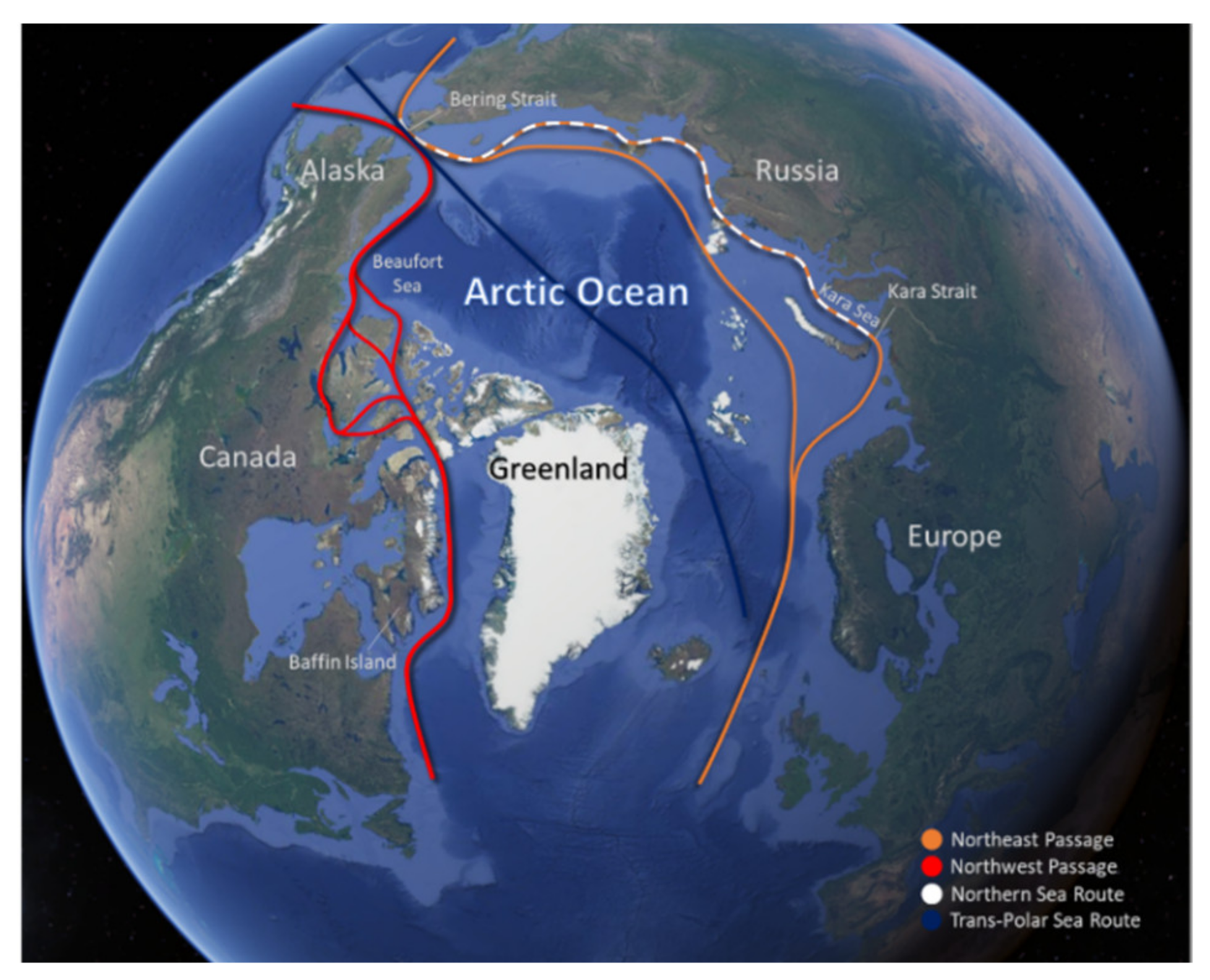
:1. Introduction
1.1. Numerical Modellings
1.2. Experimental Advances
1.3. The Aim of This Work
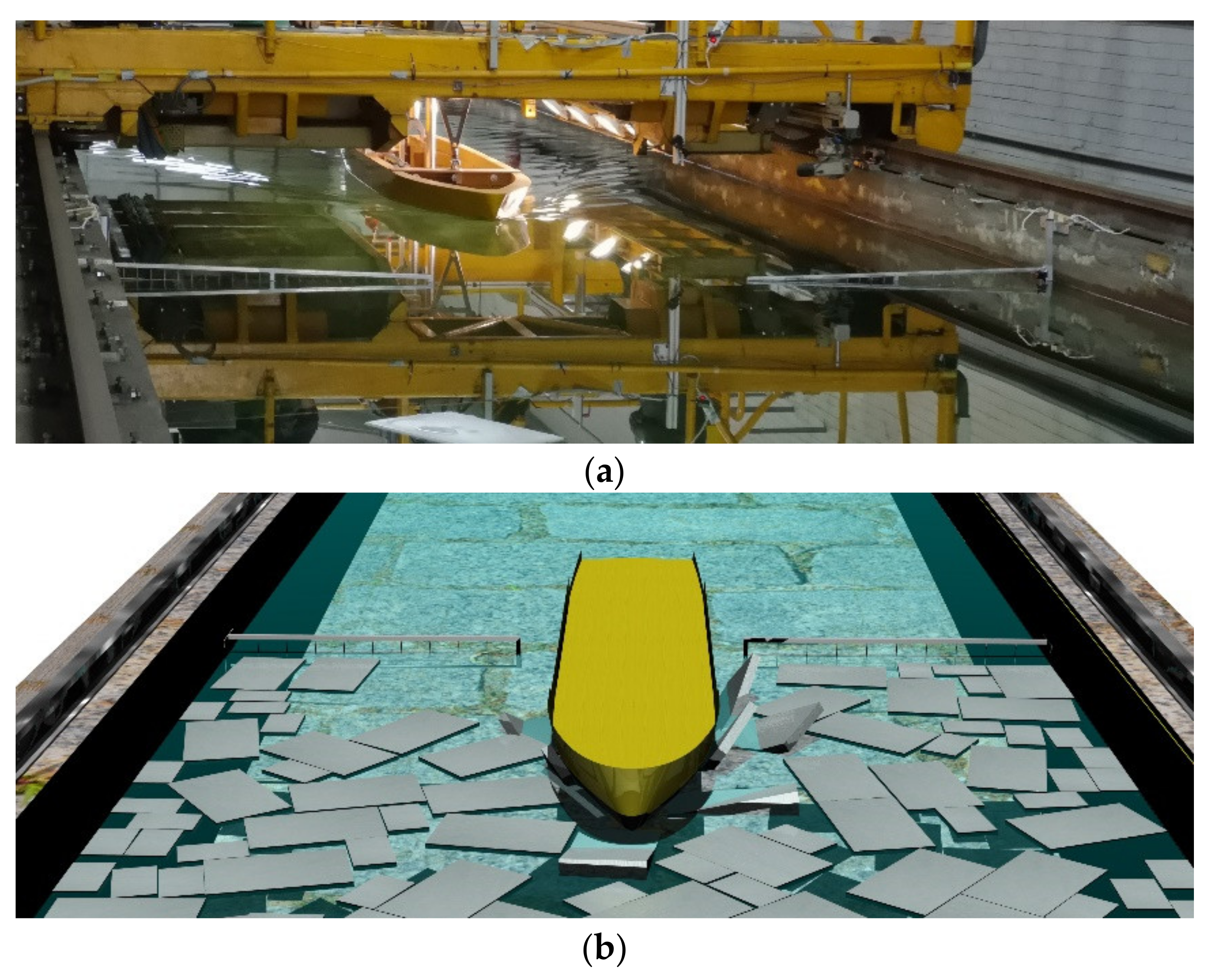
2. Experimental Facilities
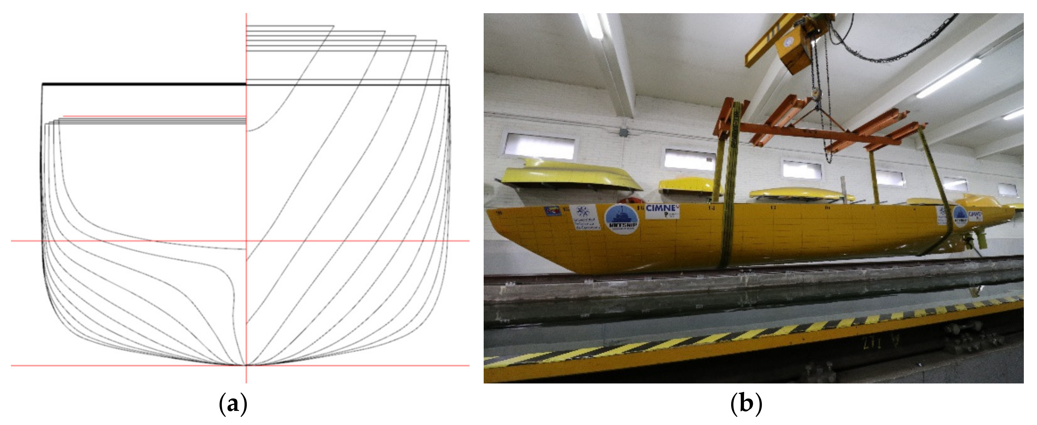
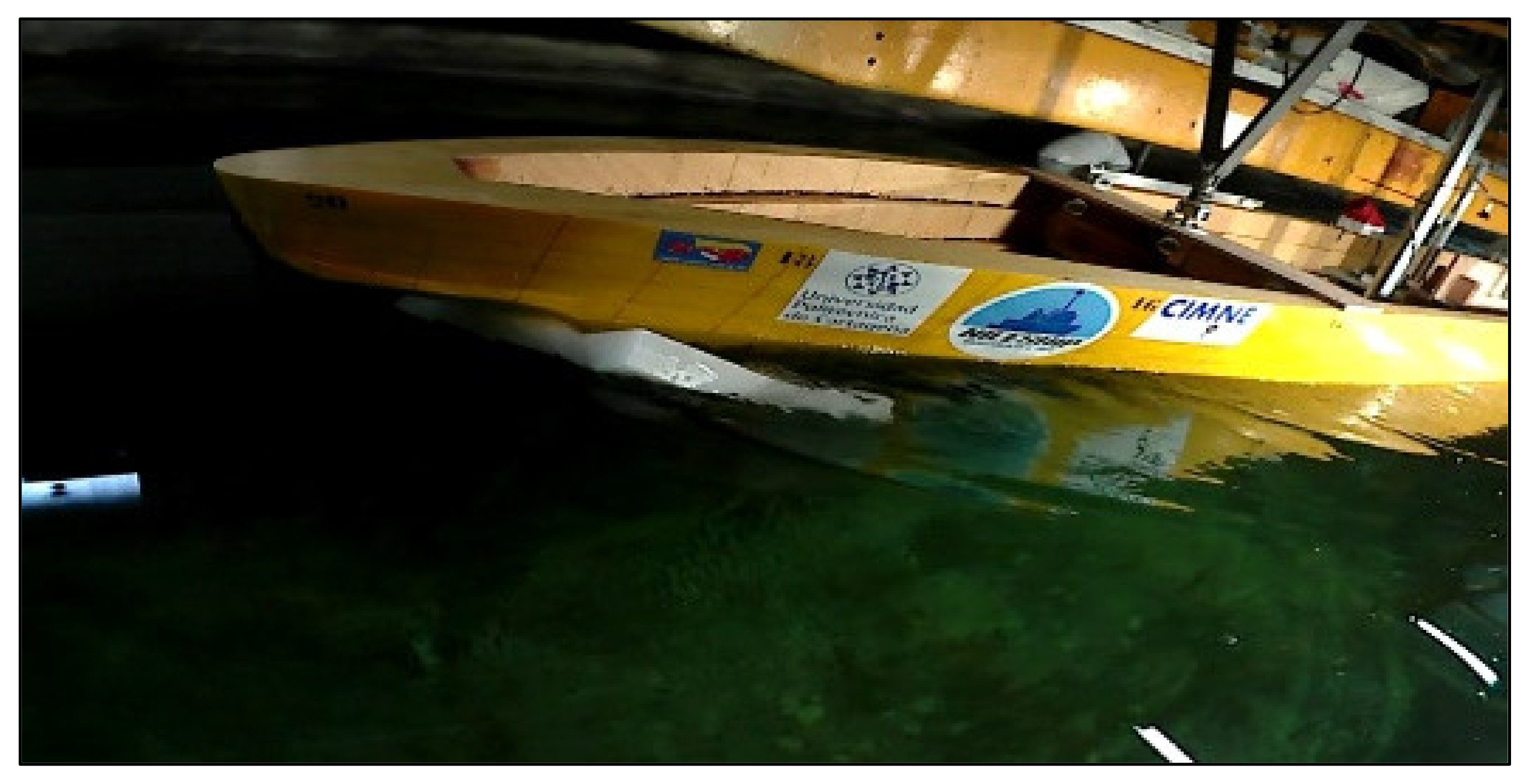
2.1. Ship Model
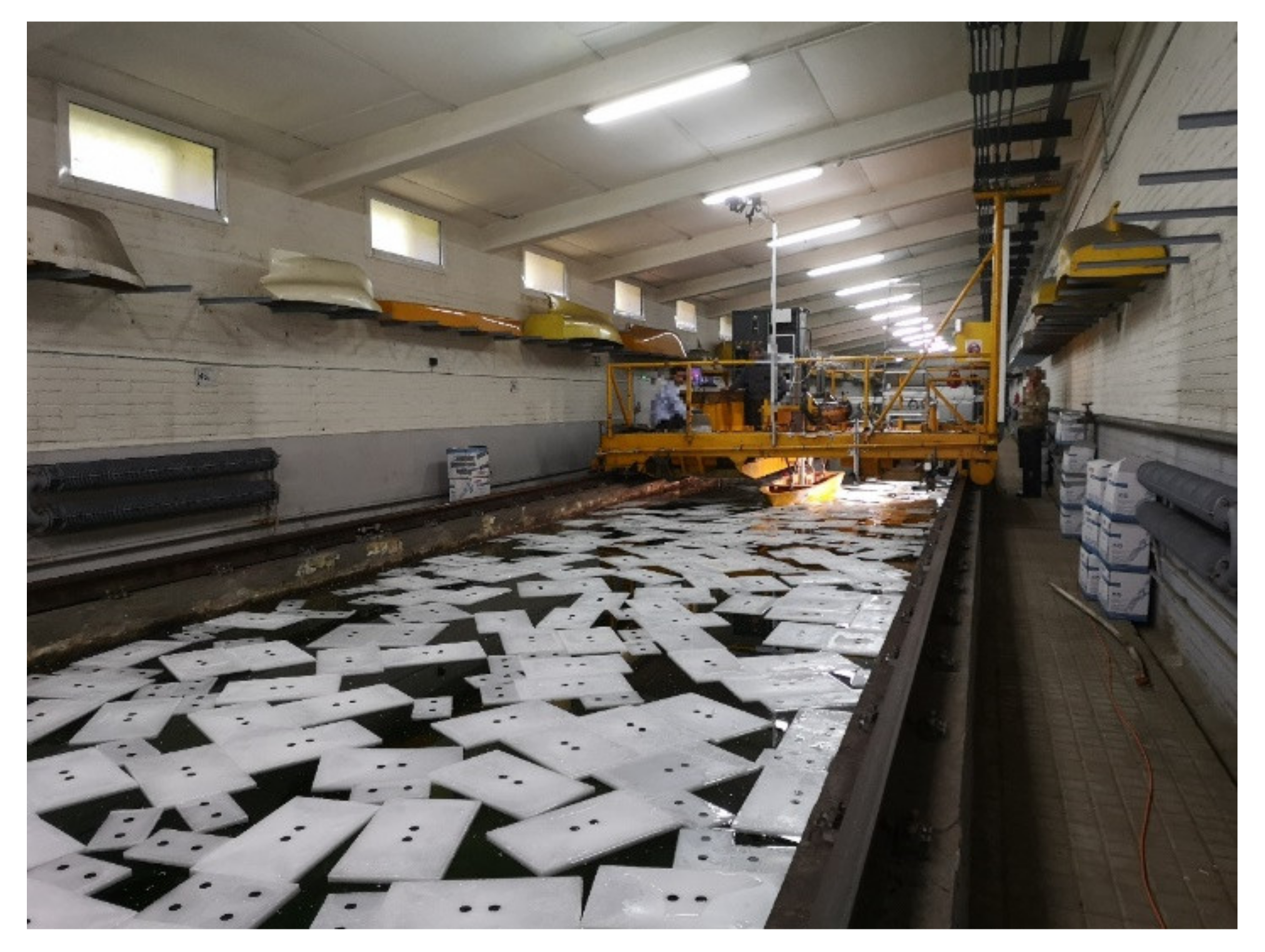
2.2. Towing Tank Facilities
2.3. Paraffin Wax as Floes
3. Experimental Campaign
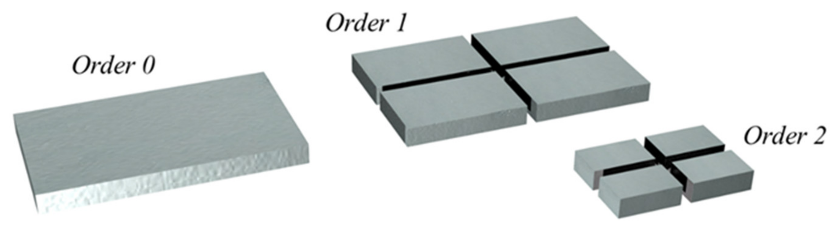
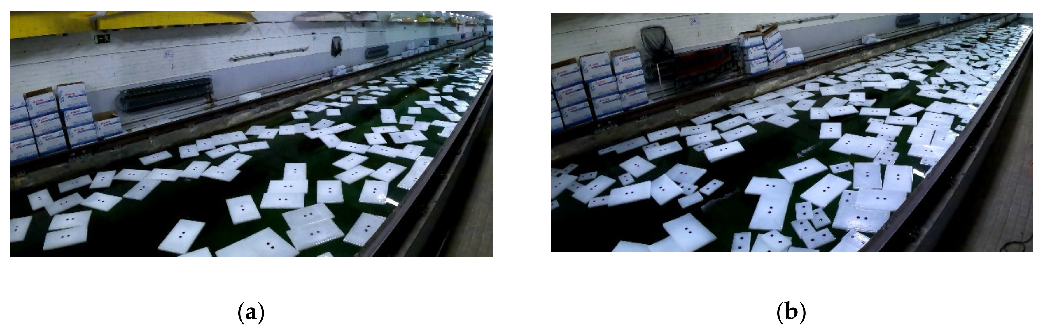
3.1. Block Distribution and Size
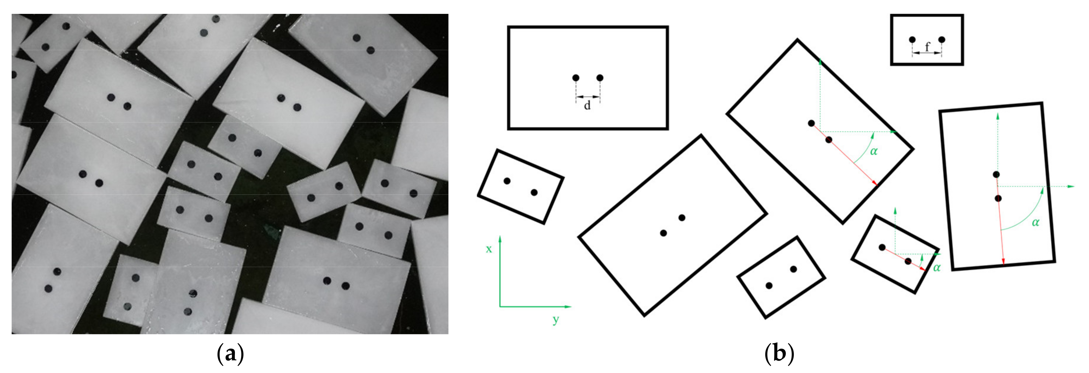
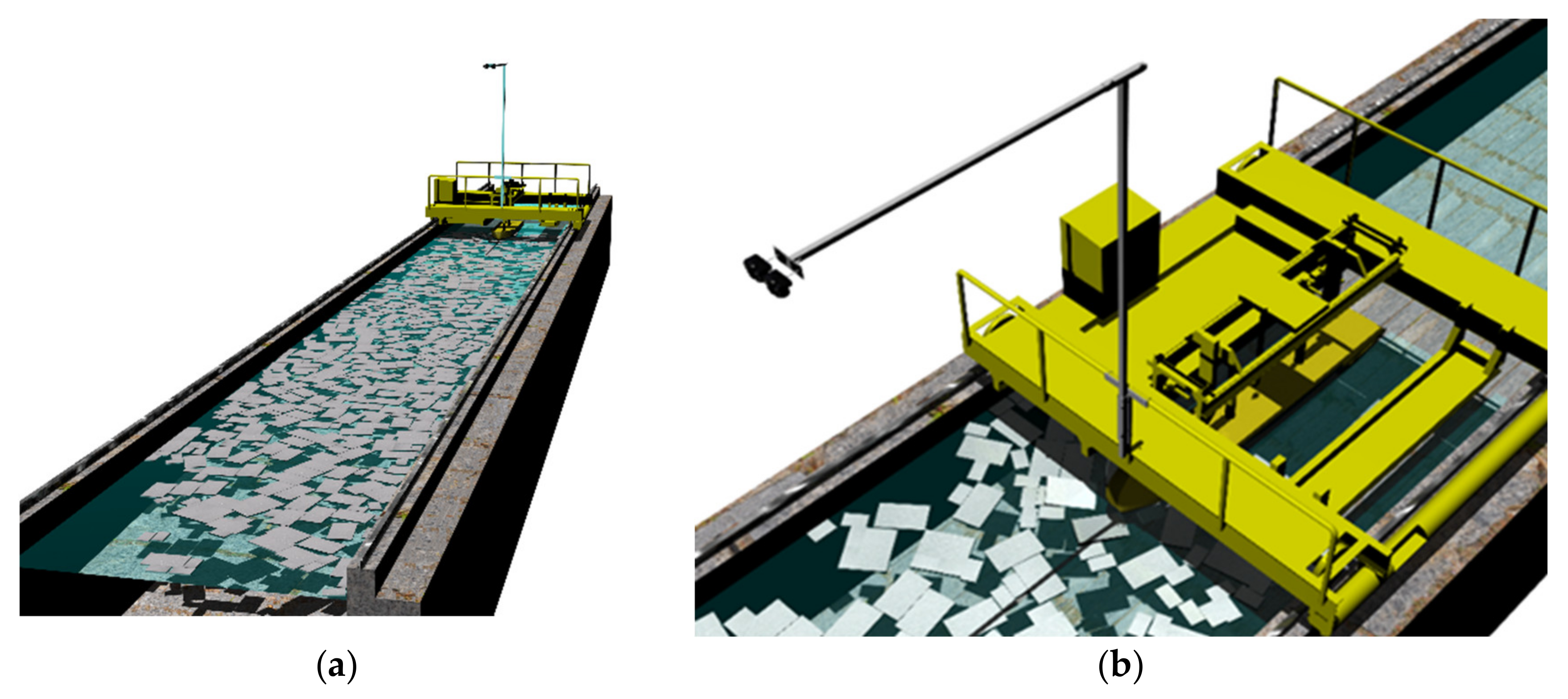
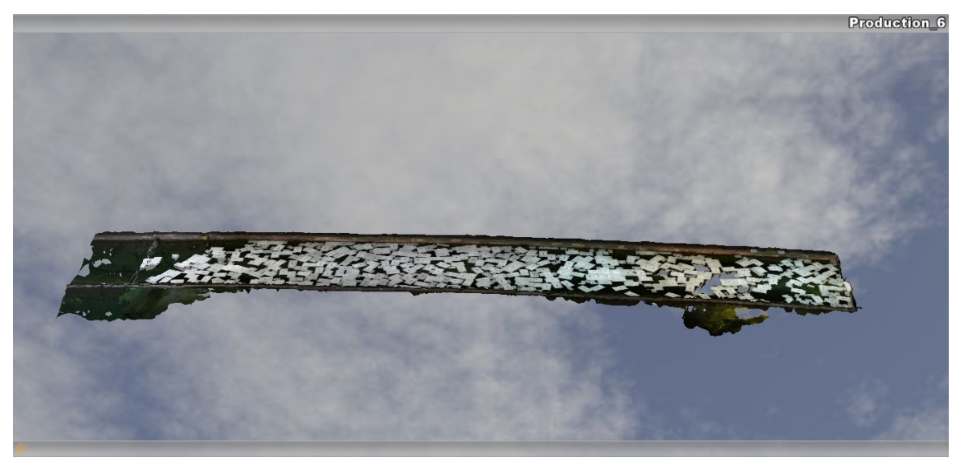
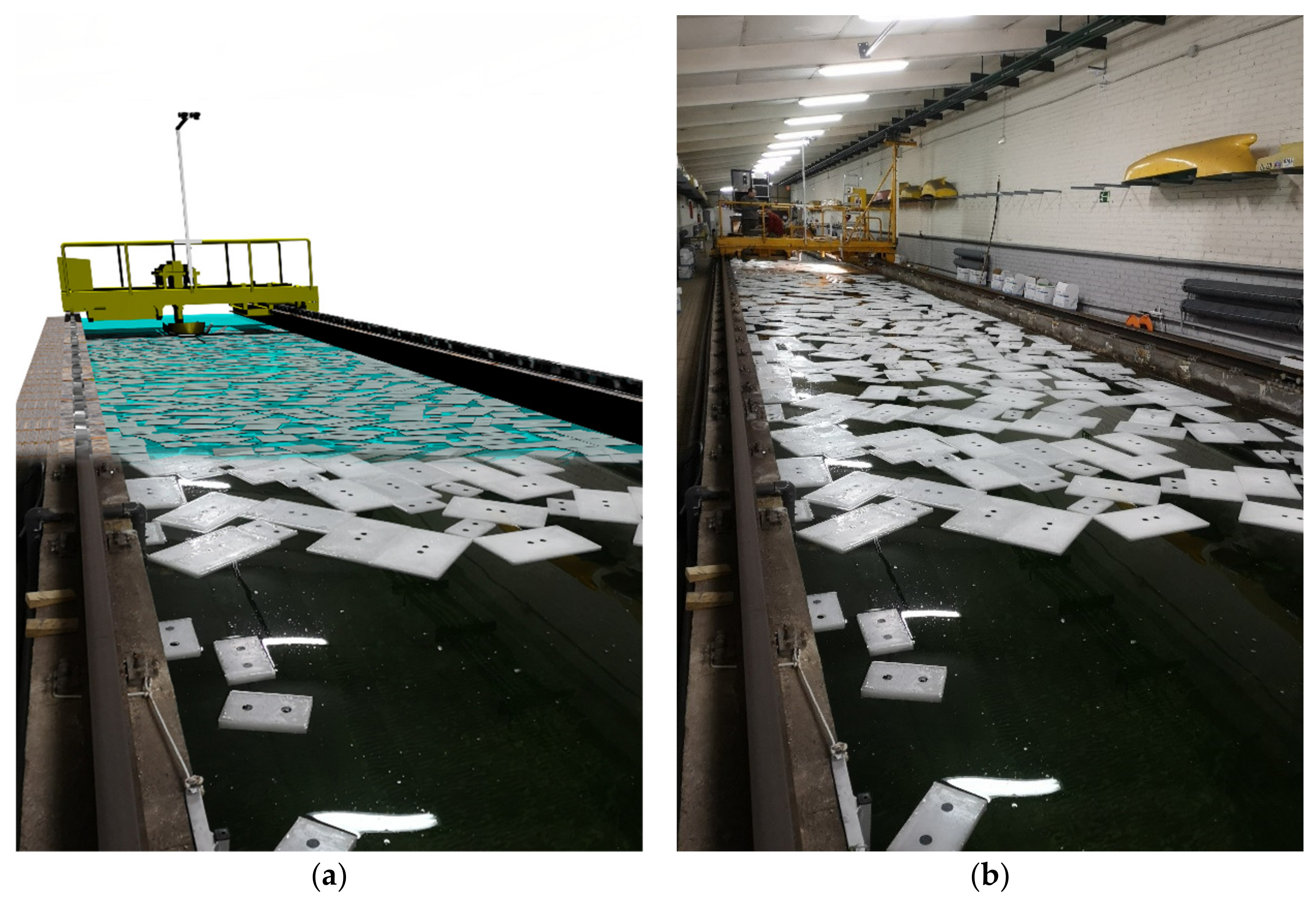
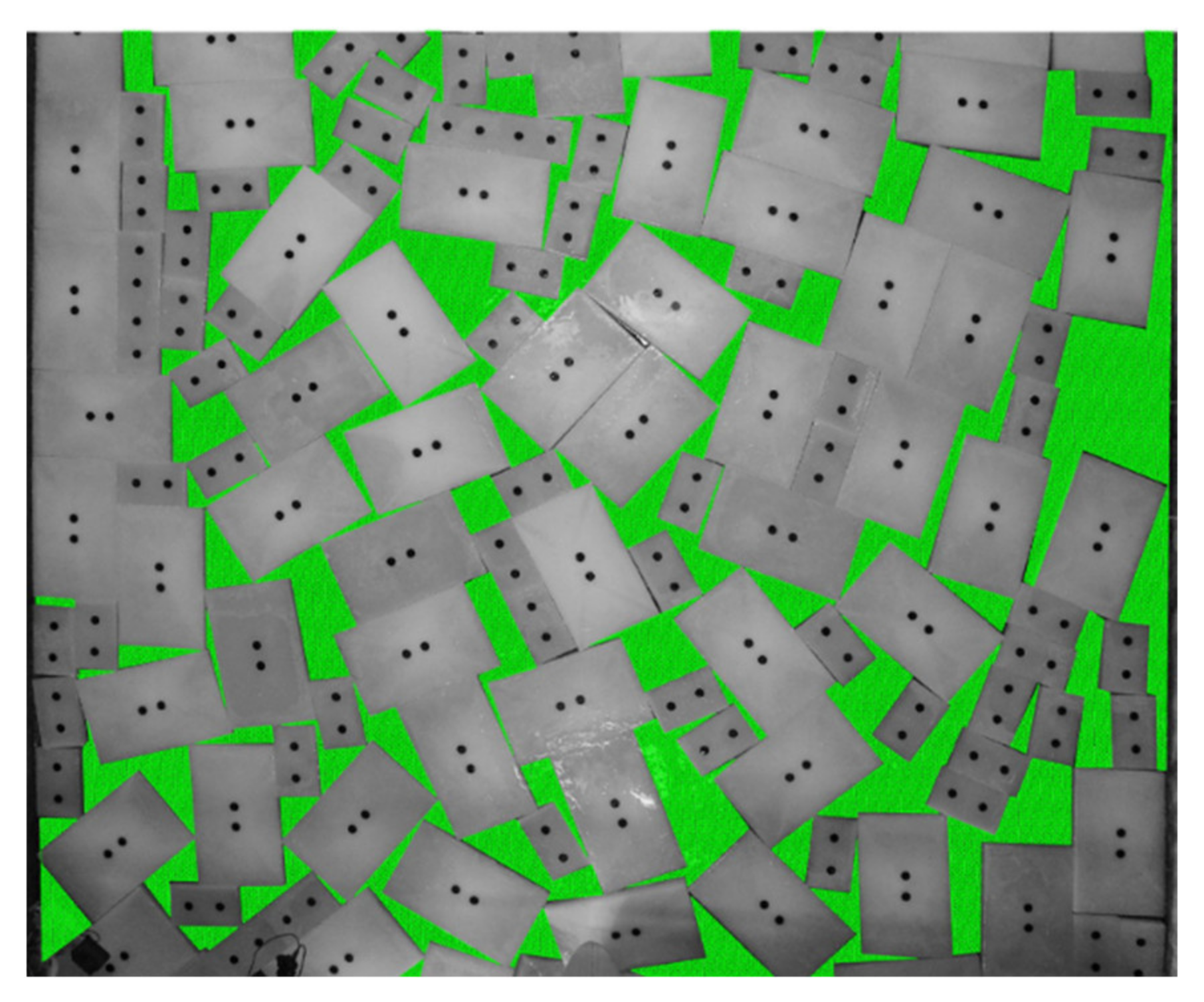
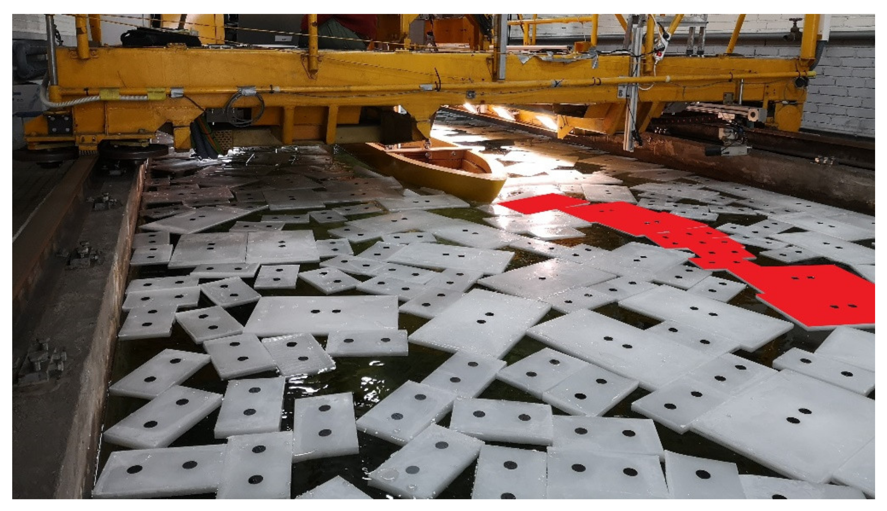
3.2. Capture System of Boundary Conditions in Initial Stationary State
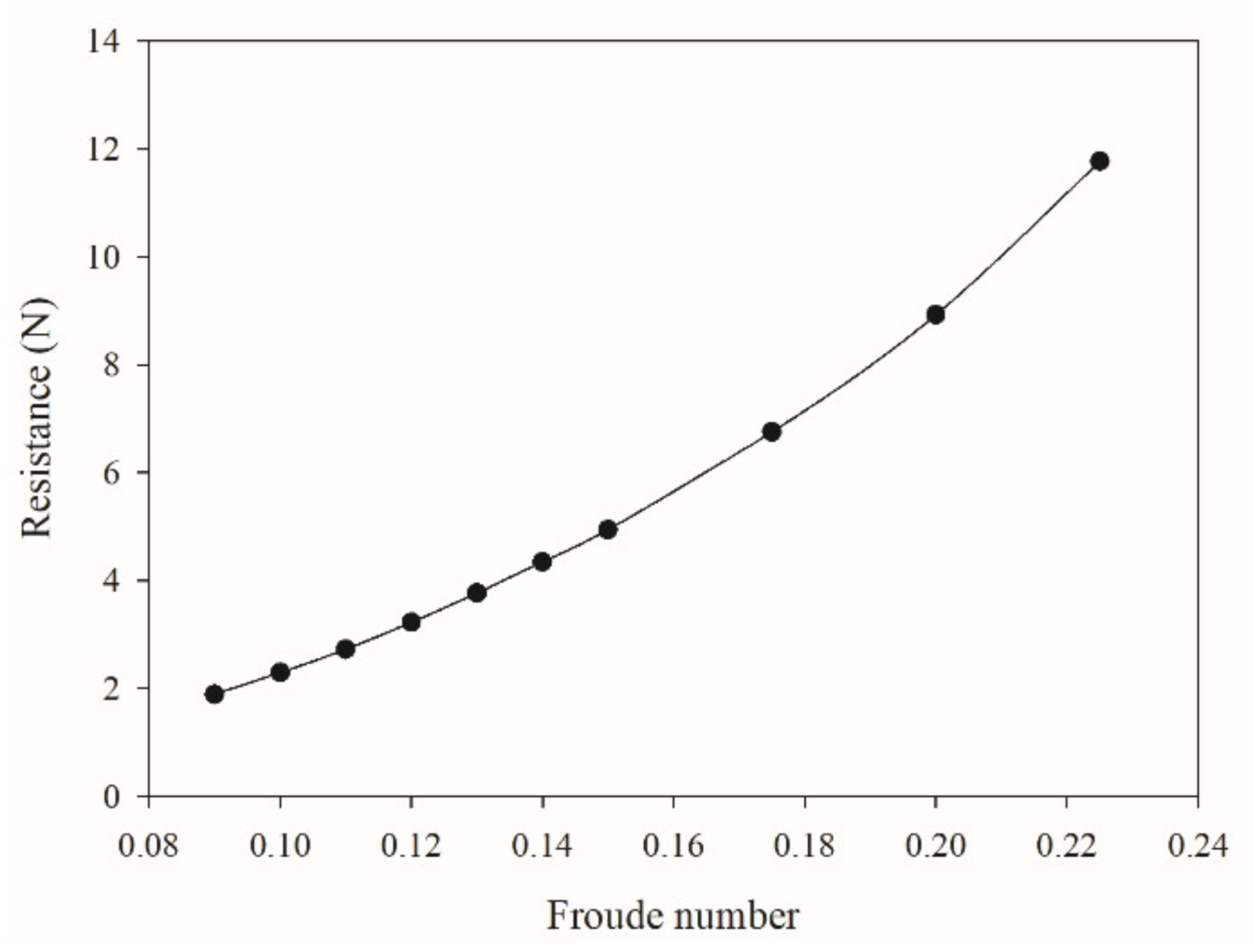
3.3. Tests
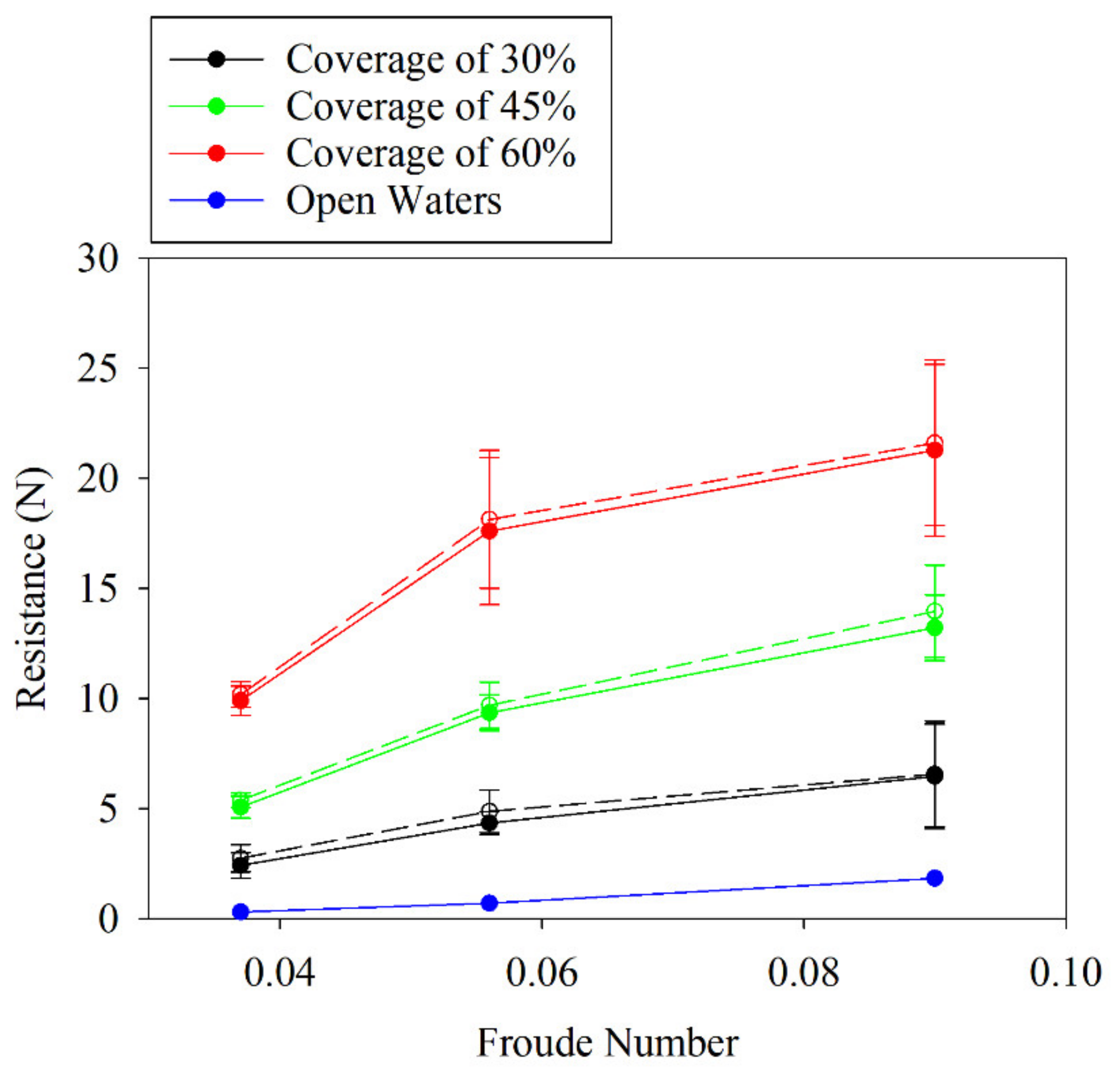
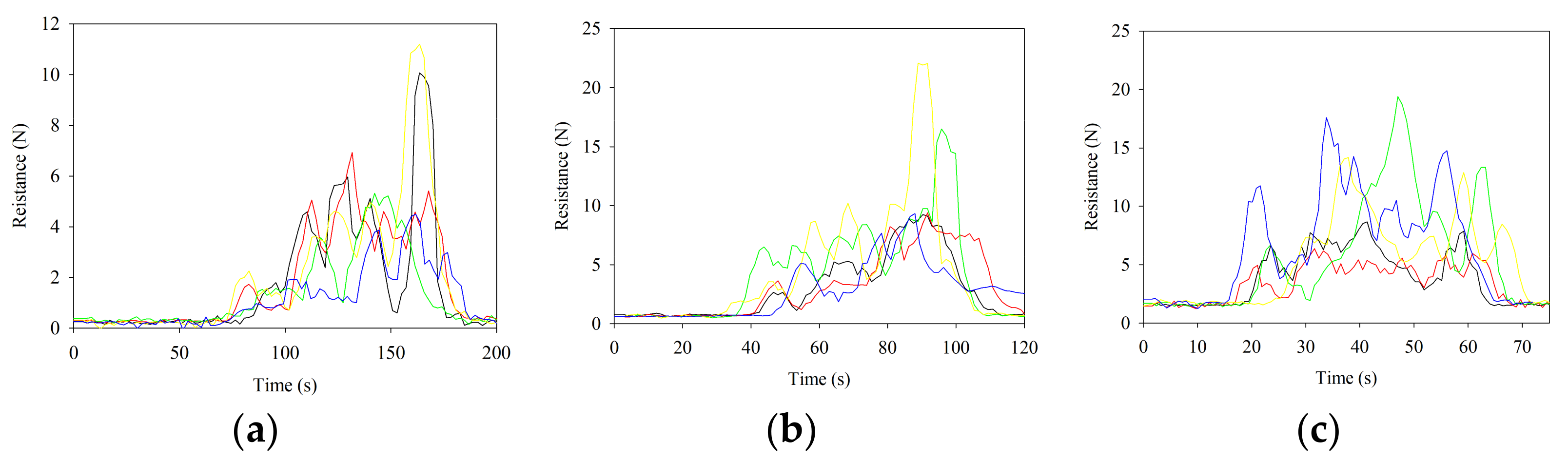
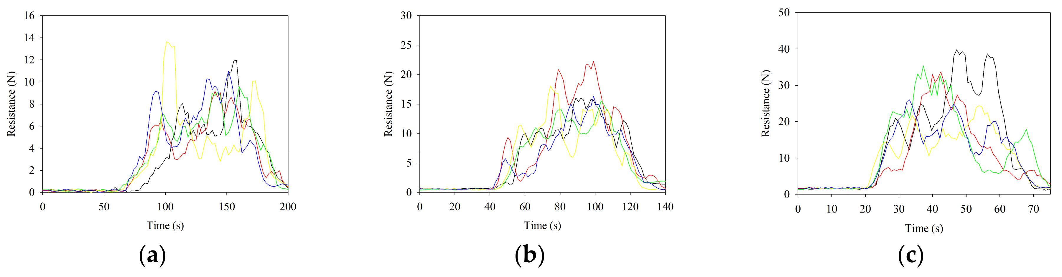
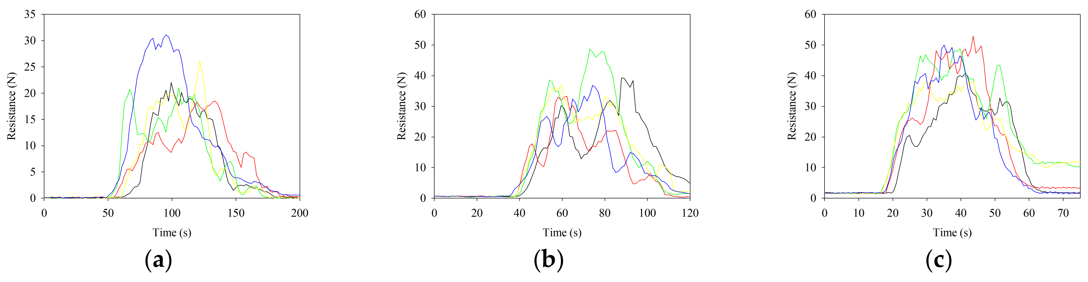
4. Results
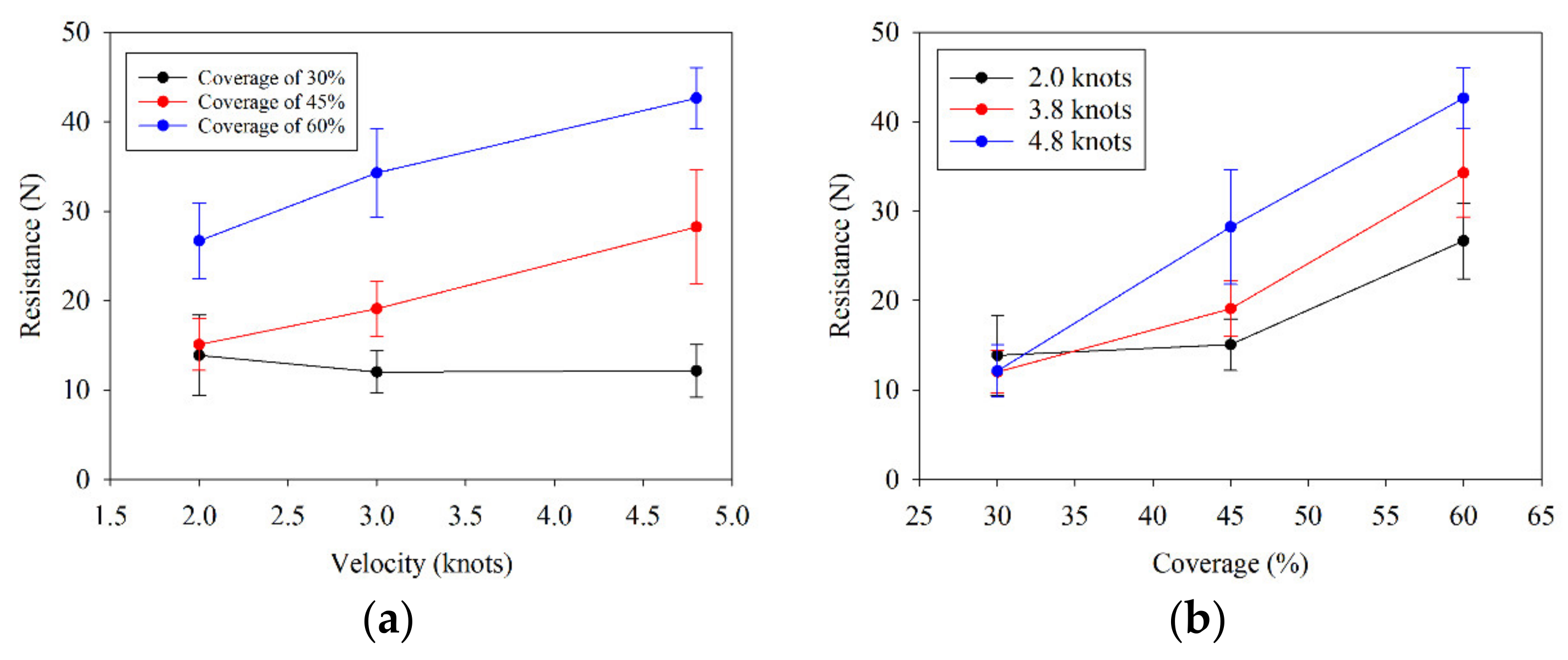
5. Discussion
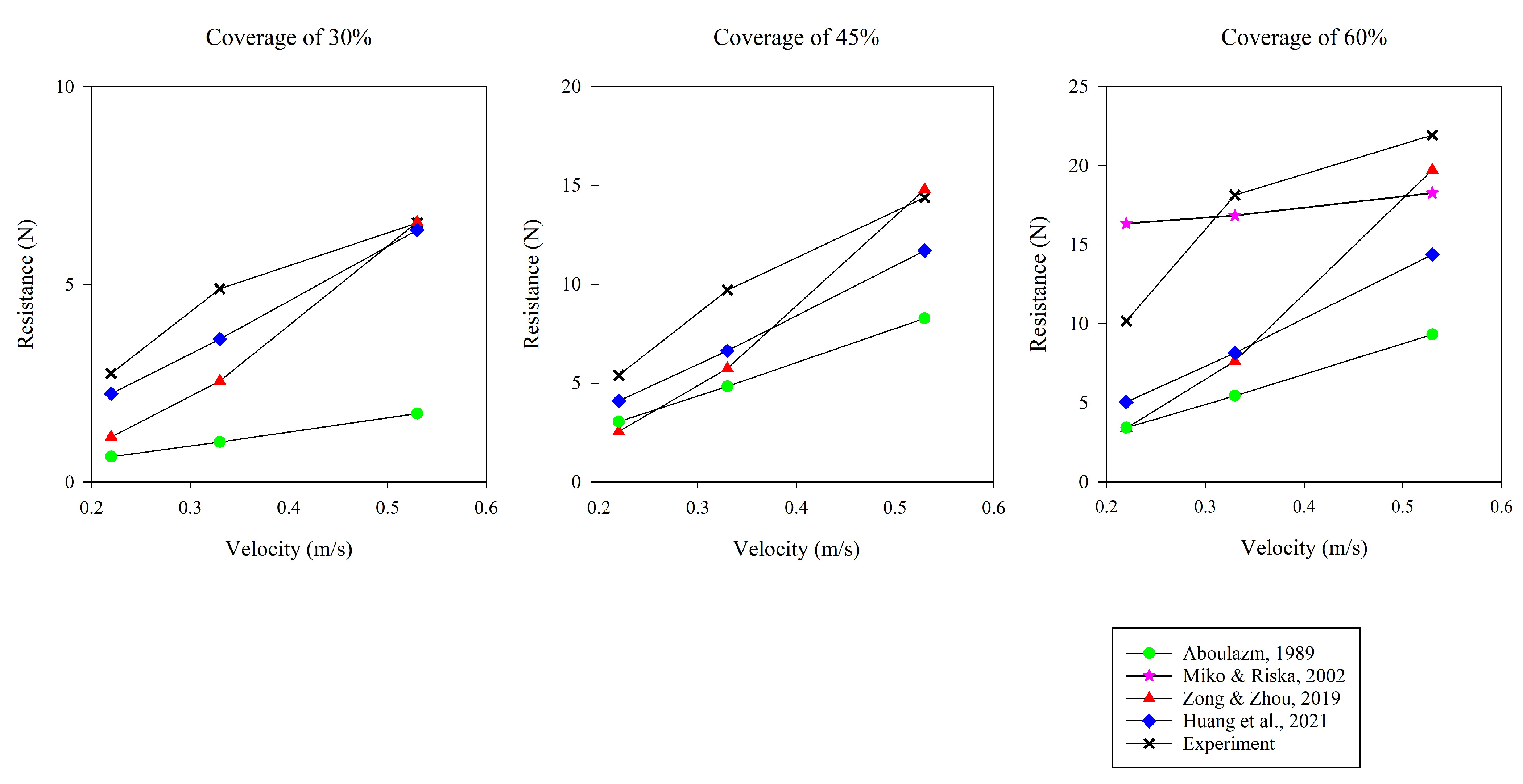
5.1. Influence of Velocity and Concentration
5.2. Influence of the Size and the Shape of Blocks
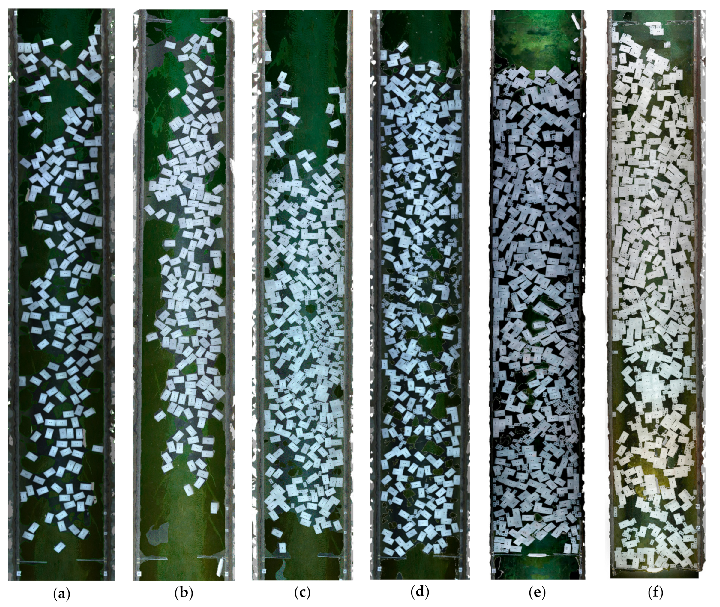
5.3. Pattern Distribution for Different Tests
6. Conclusions and Further Research
- The use of paraffin wax could be an alternative to obtain affordable solutions to study ship-block interaction during ship navigation in broken ice conditions, avoiding the sometimes high cost of ice tests.
- Photogrammetry can be used to successfully determine the initial position of blocks before each test. The information retrieved can be used then to verify and validate numerical code with floating objects on a free surface. In our case, these data are provided as a service to other researches.
- It was observed that higher concentrations above 45% give a better quality of retrieved signal. Lower concentrations give higher oscillations compared with concentrations of 45% and 60%.
- The mean resistance may be influenced by the block shape. Edge to edge contacts were common in the observations made. Large chains of blocks were noticed mainly at high concentrations. It seems reasonable that the main resistance in real conditions could be less than that obtained from this experimentation. However, the main objective was to provide valuable data for other numerical developments to study ship navigation with objects on a free surface.
- Ship-block resistance reached up to eight times open water resistance. Many other works have obtained similar results, as aforementioned.
- Bounds at the end of the ice channel produce block jams. This phenomenon increases the instantaneous ship resistance.
- The attachment phenomenon in which the largest dimension of the block is perpendicular to the bow of the ship produces an increase in the ship resistance.
- The main findings explained above are based on measurements obtained from model tests under specific conditions. The information provided, together with the block distribution figures with different coverages, should help other researches.
Supplementary Materials
Author Contributions
Funding
Institutional Review Board Statement
Informed Consent Statement
Data Availability Statement
Acknowledgments
Conflicts of Interest
References
- Intergovernmental Panel on Climate Change (IPCC). IPCC Special Report on the Ocean and Cryosphere in a Changing Climate; Pörtner, H.-O., Roberts, D.C., Masson-Delmotte, V., Zhai, P., Tignor, M., Poloczanska, E., Mintenbeck, K., Alegría, A., Nicolai, M., Okem, A., et al., Eds.; IPCC: Geneva, Switzerland, 2019; in press. [Google Scholar]
- Lasserre, F.; Beveridge, L.; Fournier, M.; Têtu, P.-H.; Huang, L. Polar seaways? Maritime transport in the Arctic: An analysis of shipowners’ intentions II. J. Transp. Geogr. 2016, 57, 105–114. [Google Scholar] [CrossRef]
- Timco, G.W. EG/AD/S: A new type of model ice for re-frigerated towing tanks. Cold Reg. Sci. Technol. 1986, 12, 175–195. [Google Scholar] [CrossRef]
- Lau, M.; Wang, J.; Lee, C. Review of ice modelling methodology. In Proceedings of the 19th International Conference on Port and Ocean Engineering under Arctic Conditions (POAC’07), Dalian, China, 27–30 June 2007; pp. 250–362. [Google Scholar]
- Lindqvist, G. A straightforward method for calculation of ice resistance of ships. In Proceedings of the 10th International Conference on Port and Ocean Engineering under Arctic Conditions (POAC’89), Lulea, Sweden, 12–16 June 1989; pp. 722–735. [Google Scholar]
- Riska, K. Performance of Merchant Vessels in Ice in the Baltic. Research Report/Winter Navigation Research Board, 52; Helsinki University of Technology, Ship Laboratory: Helsinki, Finland, 1997. [Google Scholar]
- Sandkvist, J. Conditions in Brash Ice-Covered Channels with Repeated Passages. In Proceedings of the 6th International Conference on Port and Ocean Engineering under Arctic Conditions (POAC’81), Quebec, QC, Canada, 27–31 July 1981; pp. 244–253. [Google Scholar]
- Kitazawa, T.; Ettema, R. Resistance to ship-hull motion through brash ice. Cold Reg. Sci. Technol. 1985, 10, 219–234. [Google Scholar] [CrossRef]
- Aboulazm, A.F. Repeated ice impacts and ship resistance in fragmented ice. In Proceedings of the 12th International Conference on Port and Ocean Engineering under Arctic Conditions (POAC’93), Hamburg, Germany, 17–20 August 1993; pp. 149–157. [Google Scholar]
- Englund, K. The Need of Engine Power for Merchant Vessels in Brash Ice Channels in the Baltic. Master’s Thesis, Helsinki University of Technology, Helsinki, Finland, 1996. [Google Scholar]
- Wilhelmson, M. The Resistance of a Ship in a Brash Ice Channel. Master’s Thesis, Helsinki University of Technology, Helsinki, Finland, 1996. [Google Scholar]
- Molyneux, D. Estimating performance requirements for ships navigating to and from Voisey’s bay. In Proceedings of the 18th International Conference on Port and Ocean Engineering under Arctic Conditions. (POAC’05), Potsdam, NY, USA, 26–30 June 2005; pp. 187–198. [Google Scholar]
- Grochowalski, S.; Hermanski, G. Ship Resistance and Propulsion in Ice-Covered Waters: An Experimental Study. Trans. Soc. Nav. Archit. Mar. Eng. 2011, 119, 67–92. [Google Scholar]
- Konno, A.; Saitoh, O.; Watanabe, Y. Numerical investigation of effect of channel conditions against ship resistance in brash ice channels. In Proceedings of the 21st International Conference on Port and Ocean Engineering under Arctic Conditions (POAC’11), Montréal, QC, Canada, 10–14 July 2011. [Google Scholar]
- Konno, A.; Nakane, A.; Kanamori, S. Validation of Numerical Estimation of Brash Ice Channel Resistance with Model Test. In Proceedings of the 22nd International Conference on Port and Ocean Engineering under Arctic Conditions (POAC’13), Espoo, Finland, 9–13 June 2013. [Google Scholar]
- Kim, M.-C.; Lee, S.-K.; Lee, W.-J.; Wang, J.-Y. Numerical and experimental investigation of the resistance performance of an icebreaking cargo vessel in pack ice conditions. Int. J. Nav. Archit. Ocean Eng. 2013, 5, 116–131. [Google Scholar] [CrossRef] [Green Version]
- Kim, M.-C.; Lee, W.-J.; Shin, Y.-J. Comparative study on the resistance performance of an icebreaking cargo vessel according to the variation of waterline angles in pack ice conditions. Int. J. Nav. Archit. Ocean Eng. 2014, 6, 876–893. [Google Scholar] [CrossRef] [Green Version]
- Van der Werff, S.; Brouwer, J.; Hagesteijn, G. Ship resistance validation using artificial ice. In Proceedings of the ASME 34th International Conference on Ocean, Offshore and Arctic Engineering (OMAE 2015), St. John’s, NL, Canada, 31 May–5 June 2015. [Google Scholar]
- Zhang, Q.; Skjetne, R.; Metrikin, I.; Løset, S. Image Processing for Ice Floe Analyses in Broken-ice Model Testing. Cold Reg. Sci. Technol. 2015, 111, 27–38. [Google Scholar] [CrossRef] [Green Version]
- Jeong, S.-Y.; Jang, J.; Kang, K.-J.; Kim, H.-S. Implementation of ship performance test in brash ice channel. Ocean Eng. 2017, 140, 57–65. [Google Scholar] [CrossRef]
- Guo, C.-Y.; Zhang, Z.-T.; Tian, T.-P.; Li, S.-Y.; Zhao, D.-G. Numerical Simulation on the Resistance Performance of Ice-Going Container Ship Under Brash Ice Conditions. China Ocean Eng. 2018, 32, 546–556. [Google Scholar] [CrossRef]
- Dobrodeev, A.A.; Sazonov, K.E. Ice resistance calculation method for a ship sailing via brash ice channel. In Proceedings of the 25th International Conference on Port and Ocean Engineering under Arctic Conditions (POAC’19), Delft, The Netherlands, 9–13 June 2019. [Google Scholar]
- Jeong, S.-Y.; Kim, H.-S. Study of Ship Resistance Characteristics in Pack Ice Fields. In Proceedings of the 25th International Conference on Port and Ocean Engineering under Arctic Conditions (POAC’19), Delft, The Netherlands, 9–13 June 2019. [Google Scholar]
- Van den Berg, M.; Lubbad, R.; Løset, S. The effect of ice floe shape on the load experienced by vertical-sided structures interacting with a broken ice field. Mar. Struct. 2019, 65, 229–248. [Google Scholar] [CrossRef]
- Zong, Z.; Yang, B.Y.; Sun, Z.; Zhang, G.Y. Experimental study of ship resistance in artificial ice floes. Cold Reg. Sci. Technol. 2020, 176, 103102. [Google Scholar] [CrossRef]
- Van den Berg, M.; Lubbad, R.; Løset, S. Repeatability of ice-tank tests with broken ice. Mar. Struct. 2020, 74, 102827. [Google Scholar] [CrossRef]
- CSIC. Unidad de Tecnología Marina. Consejo Superior de Investigación Científica. 2020. Available online: www.utm.csic.es (accessed on 10 February 2020).
- ITTC. ITTC Recommended Procedures and Guidelines. Testing and Extrapolation Methods Ice Testing Resistance Test in Level Ice. In Proceedings of the International Towing Tank Conference, Venice, Italy, 8–14 September 2002. [Google Scholar]
- ITTC. ITTC Recommended Procedures and Guidelines. Experimental Uncertainty Analysis for Ship Resistance in Ice Tank Testing. In Proceedings of the International Towing Tank Conference, Edinburgh, UK, 4–10 September 2005. [Google Scholar]
- WMO. Sea Ice Nomenclature. Volume 1—Terminology and Codes; 5th Session of JCOMM Expert Team on Sea Ice; World Meteorological Organization: Geneva, Switzerland, 2014. [Google Scholar]
- Toyota, T.; Takatsuji, S.; Nakayama, M. Characteristics of sea ice floe size distribution in the seasonal ice zone. Geophys. Res. Lett. 2006, 33, L02616. [Google Scholar] [CrossRef] [Green Version]
- Toyota, T.; Haas, C.; Tamura, T. Size distribution and shape properties of relatively small sea-ice floes in the Antarctic marginal ice zone in late winter. Deep Sea Res. Part II Top. Stud. Oceanogr. 2011, 58, 1182–1193. [Google Scholar] [CrossRef] [Green Version]
- CCG. Ice Navigation in Canadian Waters; Online; Canadian Coast Guard, Minister of Fisheries and Oceans: Ottawa, ON, Canada, 2012. [Google Scholar]
- McGlone, C.; Mikhail, M.-E.; Bethel, J.-S.; Mullen, R. Manual of Photogrammetry; American Society for Photogrammetry and Remote Sensing: Bethesda, MD, USA, 2004. [Google Scholar]
- Wolf, P.; Dewitt, B.; Wilkinson, B. Elements of Photogrammetry with Applications in GIS; McGraw-Hill: New York, NY, USA, 2014. [Google Scholar]
- Bentley Engineering. User Manual. ContextCapture; 3D Reality Modeling Software; Online; Bentley: Exton, PA, USA, 2020. [Google Scholar]
- Guo, C.-Y.; Xie, C.; Zhang, J.-Z.; Wang, S.; Zhao, D.G. Experimental Investigation of the Resistance Performance and Heave and Pitch Motions of Ice-Going Container Ship Under Pack Ice Conditions. China Ocean Eng. 2018, 32, 169–178. [Google Scholar] [CrossRef]
- Miko, J.; Riska, K. On the Power Requirements in the Finnish-Swedish Ice Class Rules; Research Report no. 53; Ship Laboratory, Helsinki University of Technology: Espoo, Finland, 2002. [Google Scholar]
- Zong, Z.; Zhou, L. A theoretical investigation of ship ice resistance in waters covered with ice floes. Ocean Eng. 2019, 186, 106114. [Google Scholar] [CrossRef]
- Aboulazm, A.F. Ship Resistance in Ice Floe Covered Waters. Ph.D. Thesis, Memorial University of Newfoundland, St. John’s, NL, Canada, 1989. [Google Scholar]
- Huang, L.; Li, Z.; Ryan, C.; Ringsberg, J.W.; Pena, B.; Li, M.; Ding, L.; Thomas, G. Ship resistance when operating in floating ice floes: Derivation, validation, and application of an empirical equation. Mar. Struct. 2021, 79, 103057. [Google Scholar] [CrossRef]
- Cho, S.-R.; Jeong, S.-Y.; Lee, S. Development of effective model test in pack ice conditions of square-type ice model basin. Ocean Eng. 2013, 67, 35–44. [Google Scholar] [CrossRef]


| Parameter | Full Scale | Model |
|---|---|---|
| Length overall, LOA (m) | 82.588 | 3.854 |
| Waterline length, Lwl (m) | 76.791 | 3.583 |
| Breadth, B (m) | 14.591 | 0.681 |
| Depth, D (m) | 12.102 | 0.565 |
| Draught, T (m) | 4.421 | 0.207 |
| Full load displacement, | 2725.86 | 0.277 |
| Metacentric height, GM (m) | − | 0.186 |
| Pitch radii of gyration, Rxx (m) | − | 0.821 |
| Vertical distance to center of gravity from baseline, KG (m) | − | 0.157 |
| Longitudinal distance to center of gravity from , LCG (m) | 34.867 | 1.627 |
| Block coefficient, (–) | 0.542 | 0.542 |
| Water plane coefficient, (–) | 0.806 | 0.806 |
| Mid-ship section coefficient, (–) | 0.863 | 0.863 |
| Model scale, (–) | − | 1:21.43 |
| Parameter | Value | Units |
|---|---|---|
| Density | 830 | kg/m3 |
| Type | Macro-crystalline | (–) |
| Oil percentage (maximum) | 0.5 | % |
| Shape | Rectangular | (–) |
| Averaged thickness | 40 mm | (–) |
| Friction coefficient hull-floe | 0.25 | (–) |
| Parameter | Value | Unit |
|---|---|---|
| Fragility coefficient (f) | 0.6 | (–) |
| Mean thickness | 40 | mm |
| Percentage of the largest paraffin wax blocks | 80 | % |
| Mean length of the largest blocks | 484 | mm |
| Mean breath of the largest blocks | 295 | mm |
| Mean length of the smallest blocks | 242 | mm |
| Mean breath of the smallest blocks | 148 | mm |
| Coverag (%) | Larger Size (Units) | Smaller Size (Units) | Area Covered (m2) |
|---|---|---|---|
| 30 | 207 | – | 29.6 |
| 45 | 251 | 240 | 44.4 |
| 60 | 447 | 429 | 79.1 |
| Coverage (%) | Average (N) | Standard Dev. (N) | Variance (N2) | RMS (N) | Uncertainty (N) |
|---|---|---|---|---|---|
| 30 | 2.746 | 7.335 | 62.510 | 7.884 | 0.983 |
| 45 | 5.394 | 7.080 | 52.316 | 8.924 | 0.952 |
| 60 | 10.174 | 11.547 | 134.396 | 15.445 | 0.791 |
| Coverage (%) | Average (N) | Standard Dev. (N) | Variance (N2) | RMS (N) | Uncertainty (N) |
|---|---|---|---|---|---|
| 30 | 4.884 | 7.100 | 57.894 | 8.669 | 0.952 |
| 45 | 9.689 | 8.434 | 75.396 | 12.866 | 1.134 |
| 60 | 18.142 | 17.142 | 298.700 | 24.948 | 1.896 |
| Coverage (%) | Average (N) | Standard Dev. (N) | Variance (N2) | RMS (N) | Uncertainty (N) |
|---|---|---|---|---|---|
| 30 | 6.551 | 5.962 | 36.736 | 0.902 | 1.734 |
| 45 | 14.396 | 14.141 | 212.725 | 20.221 | 2.303 |
| 60 | 21.927 | 23.732 | 420.834 | 27.243 | 2.707 |
| Parameter | Value | Unit |
|---|---|---|
| Porosity, p | 0.005 | (–) |
| Constant of passive stress, Kp | 0.5 | (–) |
| Coefficient of lateral stress at rest, Ko | 0.5 | (–) |
| Length of parallel midbody at the waterline, Lpar | 41.3 | m |
| Buttock angle, | 66.7 | deg |
| Waterplane entrance angle, | 20 | deg |
| Waterplane area of foreship, Awp | 315 | m2 |
| Slope angle and the sidewall, | 22.6 | deg |
| Added mass coefficient, Ca | 1.6 | (–) |
Publisher’s Note: MDPI stays neutral with regard to jurisdictional claims in published maps and institutional affiliations. |
© 2022 by the authors. Licensee MDPI, Basel, Switzerland. This article is an open access article distributed under the terms and conditions of the Creative Commons Attribution (CC BY) license (https://creativecommons.org/licenses/by/4.0/).
Share and Cite
Gutiérrez-Romero, J.E.; Ruiz-Capel, S.; Esteve-Pérez, J.; Zamora-Parra, B.; Luna-Abad, J.P. Methodology Based on Photogrammetry for Testing Ship-Block Resistance in Traditional Towing Tanks: Observations and Benchmark Data. J. Mar. Sci. Eng. 2022, 10, 246. https://doi.org/10.3390/jmse10020246
Gutiérrez-Romero JE, Ruiz-Capel S, Esteve-Pérez J, Zamora-Parra B, Luna-Abad JP. Methodology Based on Photogrammetry for Testing Ship-Block Resistance in Traditional Towing Tanks: Observations and Benchmark Data. Journal of Marine Science and Engineering. 2022; 10(2):246. https://doi.org/10.3390/jmse10020246
Chicago/Turabian StyleGutiérrez-Romero, José Enrique, Samuel Ruiz-Capel, Jerónimo Esteve-Pérez, Blas Zamora-Parra, and Juan Pedro Luna-Abad. 2022. "Methodology Based on Photogrammetry for Testing Ship-Block Resistance in Traditional Towing Tanks: Observations and Benchmark Data" Journal of Marine Science and Engineering 10, no. 2: 246. https://doi.org/10.3390/jmse10020246
APA StyleGutiérrez-Romero, J. E., Ruiz-Capel, S., Esteve-Pérez, J., Zamora-Parra, B., & Luna-Abad, J. P. (2022). Methodology Based on Photogrammetry for Testing Ship-Block Resistance in Traditional Towing Tanks: Observations and Benchmark Data. Journal of Marine Science and Engineering, 10(2), 246. https://doi.org/10.3390/jmse10020246