
Numerical Investigation on the Dynamics of Mixture Transport in Flexible Risers during Deep-Sea Mining


Abstract
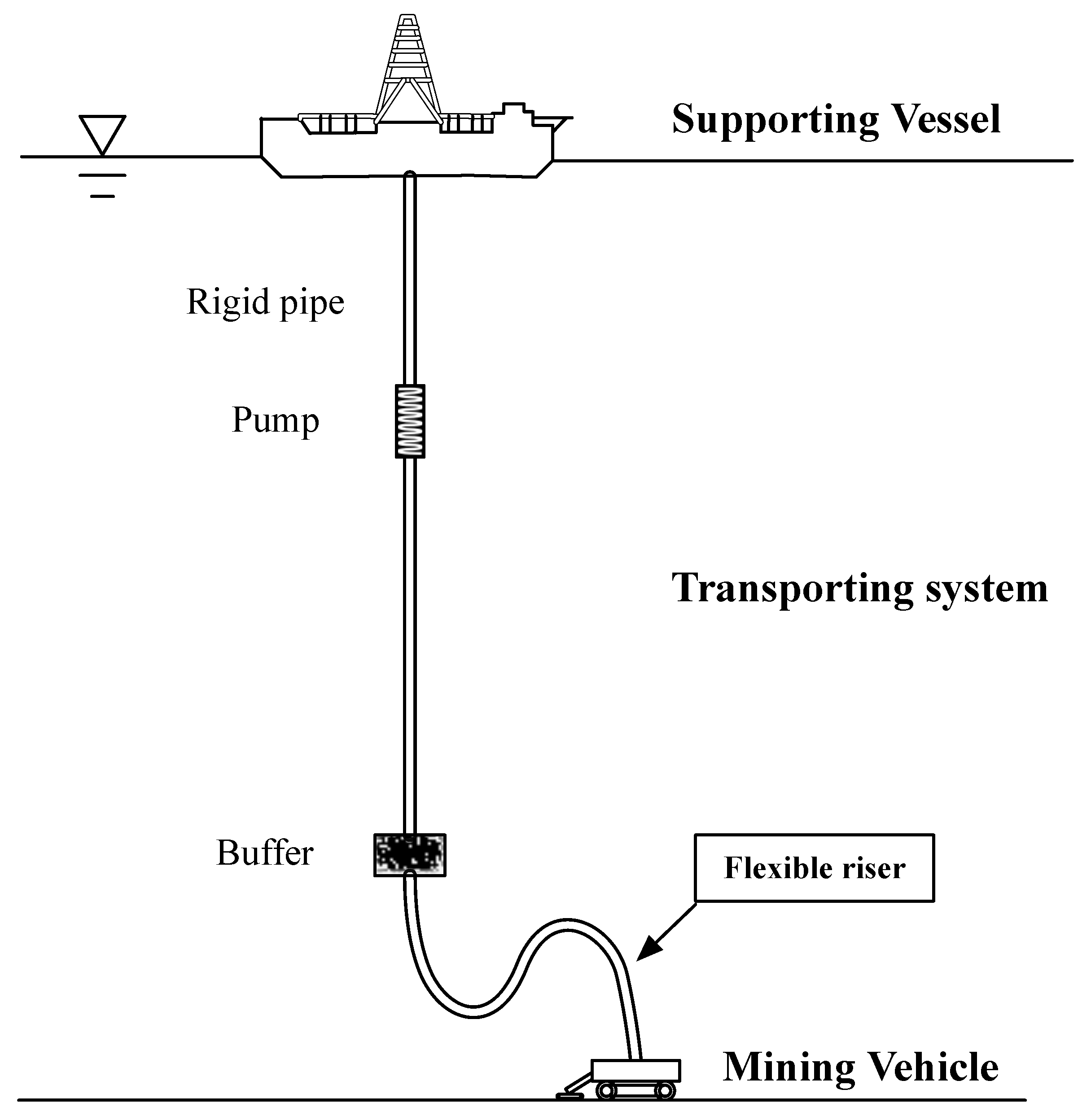
1. Introduction
2. Mathematical Formulas
2.1. Governing Equations
2.2. Fluid-Particle Interaction
2.3. Contact Model for Particle–Particle and Particle–Wall Collisions
3. Numerical Model
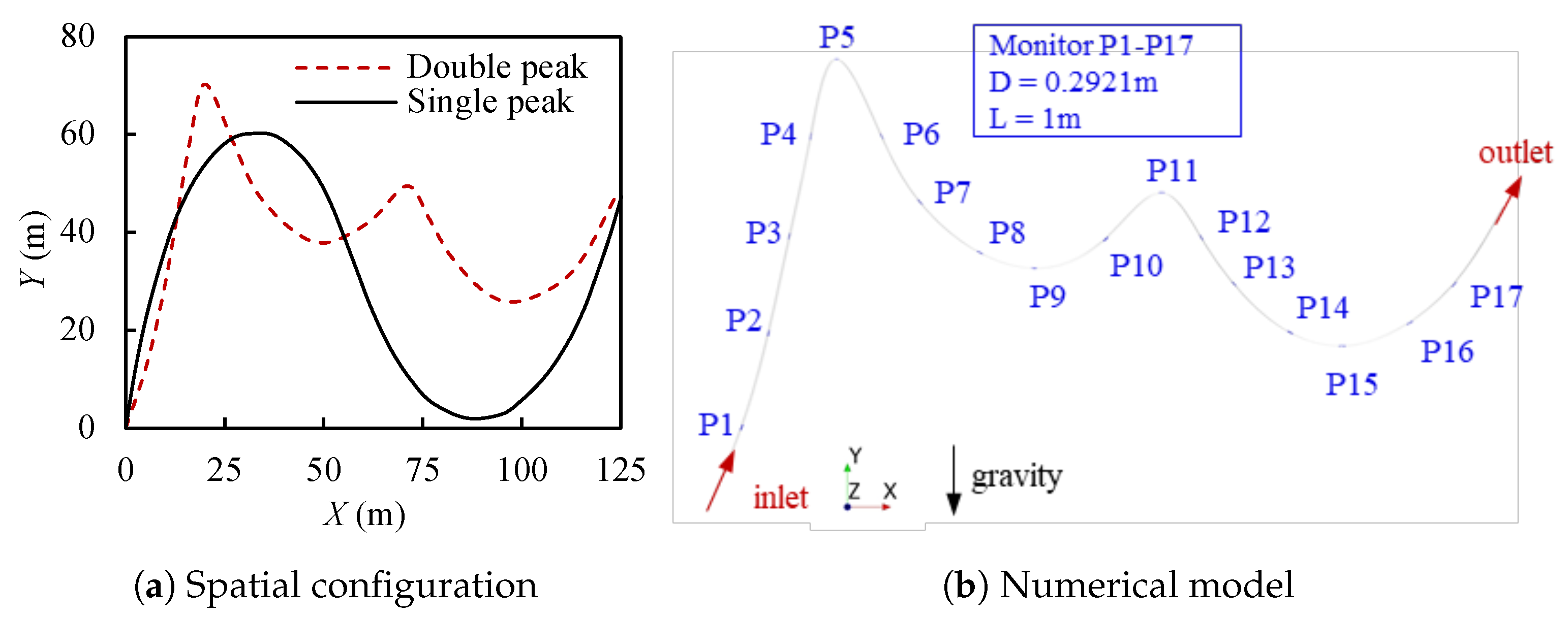
3.1. Overview of Numerical Model
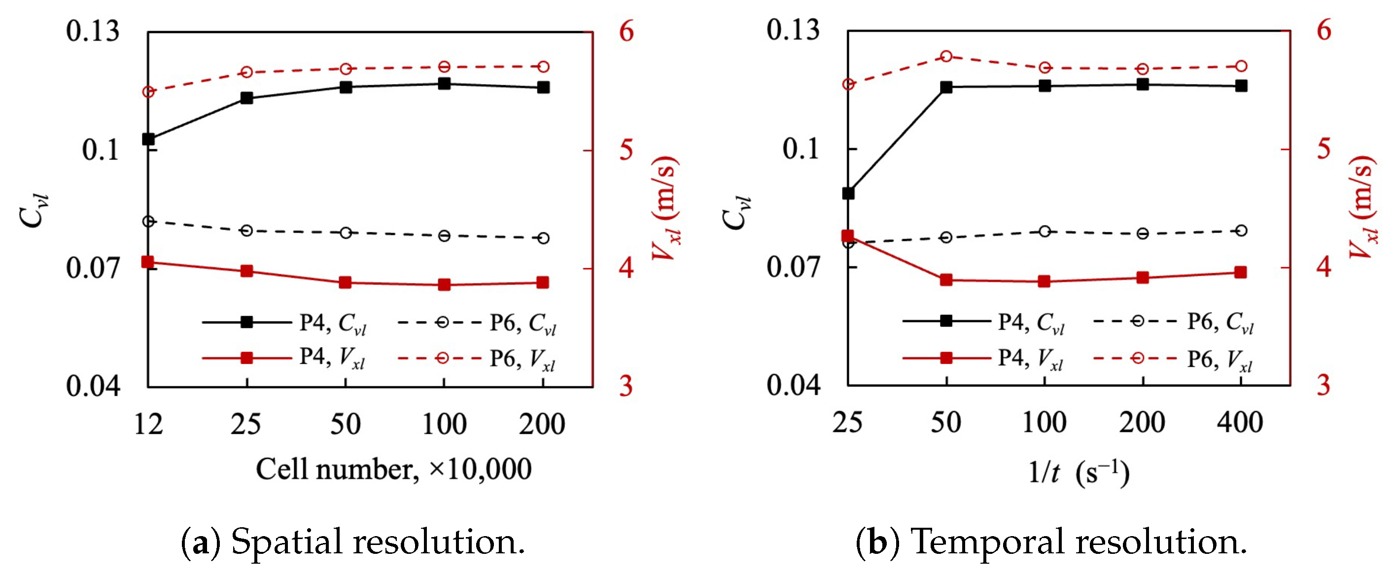
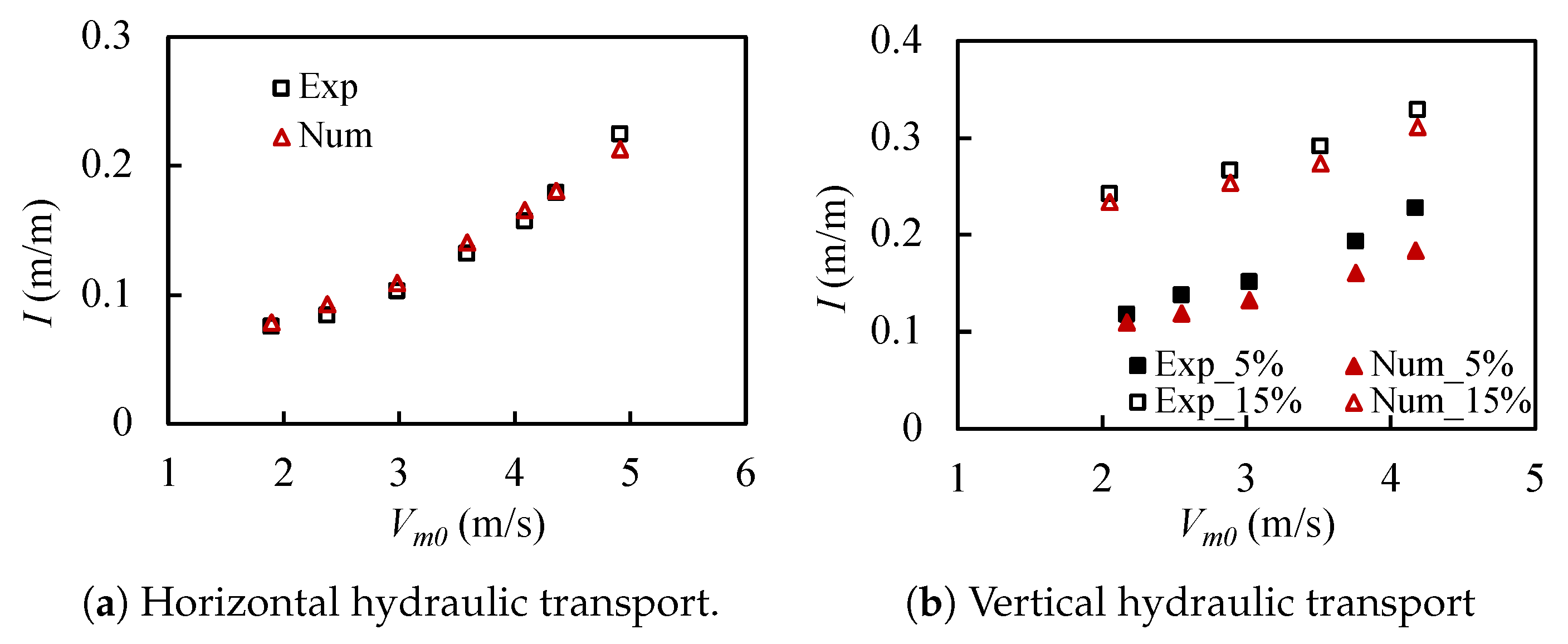
3.2. Convergence Study and Method Validation
4. Results and Discussion
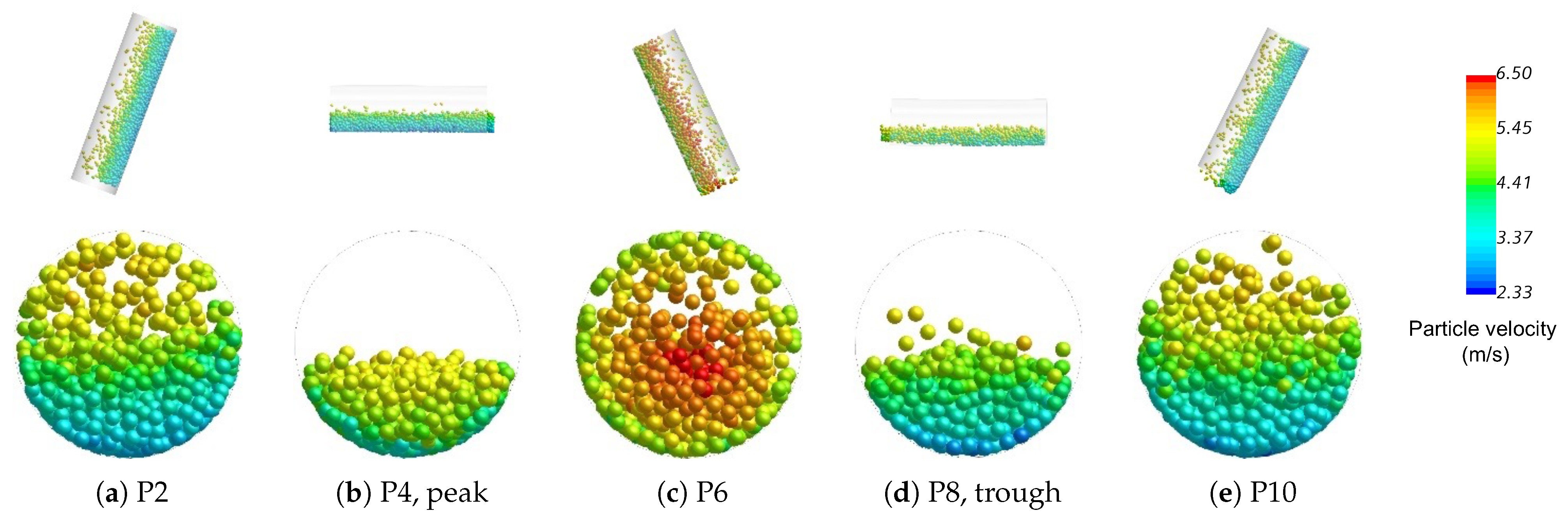
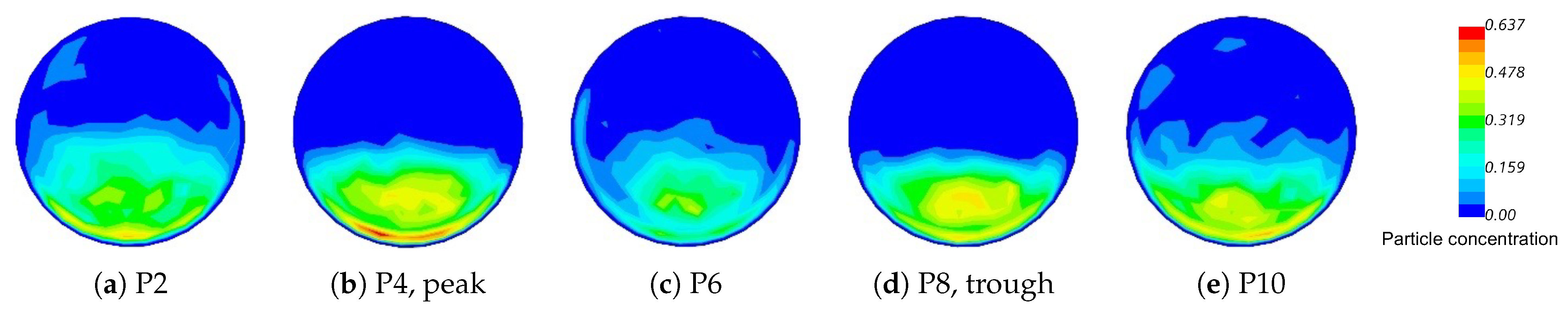
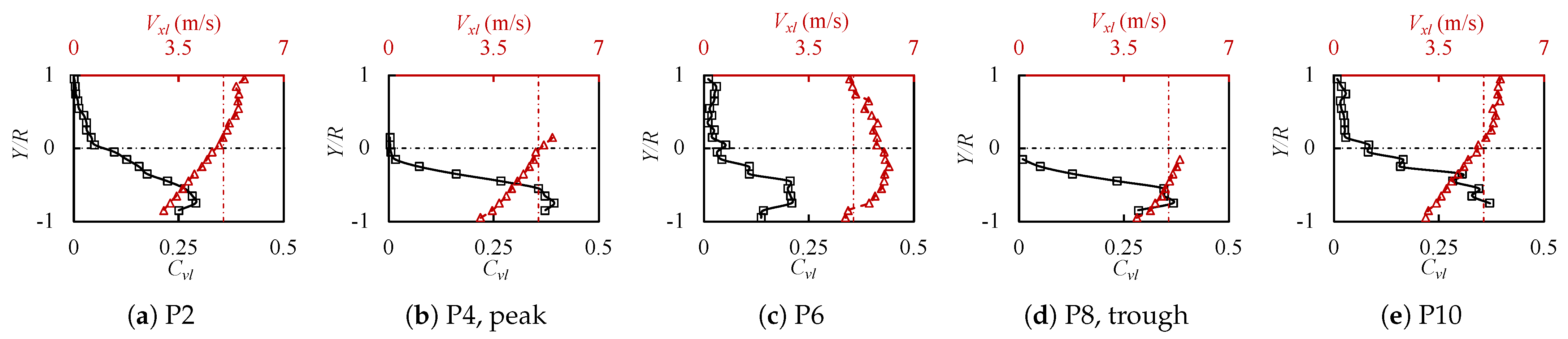
4.1. Overall Description of the Mixture Transport
4.2. Effects of Feeding Concentration and Mixture Transport Velocity
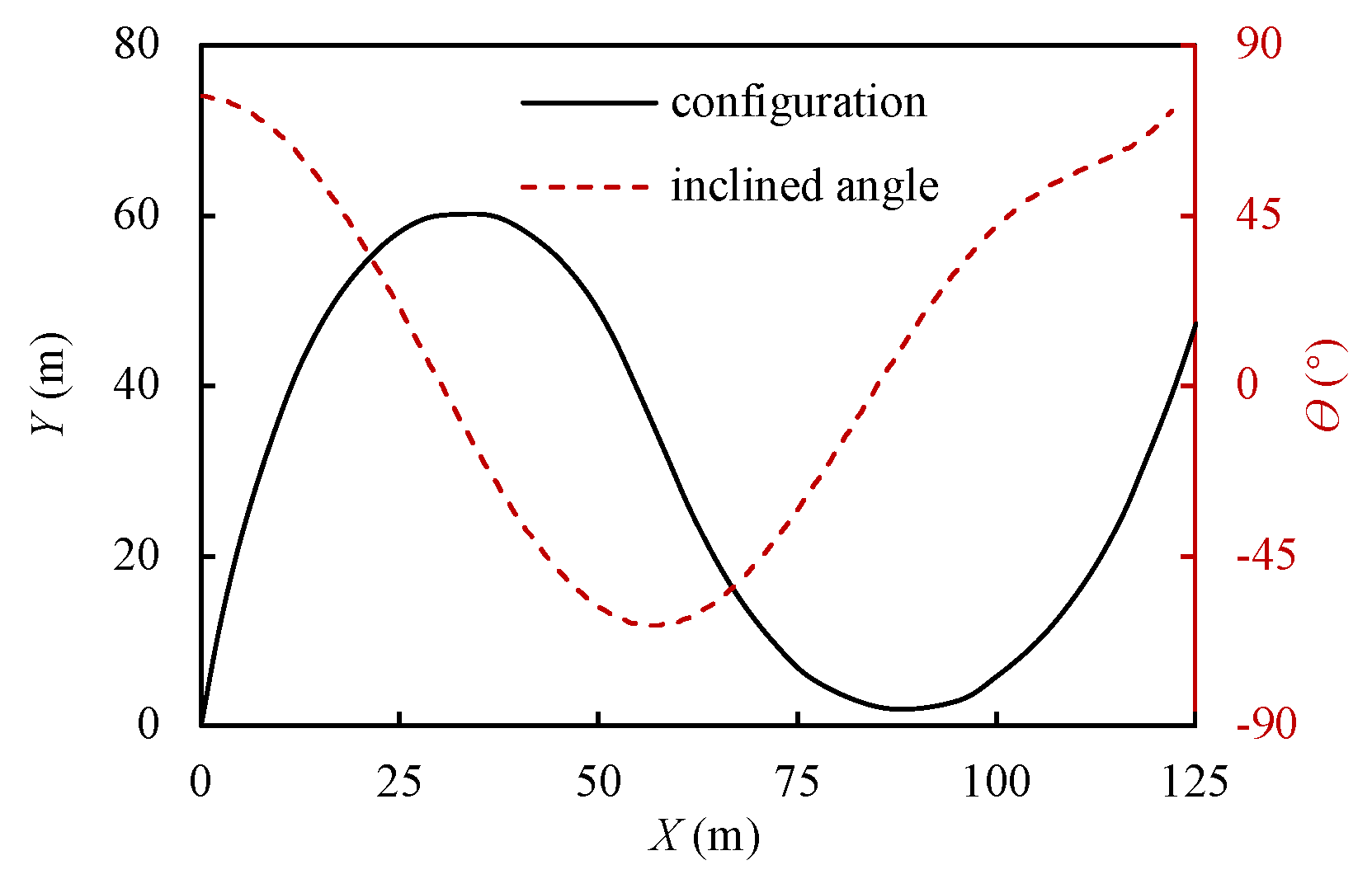
4.3. Influence of Riser Configuration
5. Conclusions
Author Contributions
Funding
Institutional Review Board Statement
Informed Consent Statement
Data Availability Statement
Acknowledgments
Conflicts of Interest
References
- Murray, J.; Renard, A.F. Report on Deep-Sea Deposits Based on the Specimens Collected during the Voyage of H.M.S. Challenger in the Years 1872 to 1876; John Menzies and Co.: Edinburgh, UK, 1891; pp. 184–186. [Google Scholar]
- Toro, N.; Robles, P.; Jeldres, R.I. Seabed mineral resources, an alternative for the future of renewable energy: A critical review. Ore Geol. Rev. 2020, 126, 103699. [Google Scholar] [CrossRef]
- Hannington, M.; Petersen, S.; Kratschell, A. Subsea mining moves closer to shore. Nat. Geosci. 2017, 10, 158–159. [Google Scholar] [CrossRef]
- Leng, D.; Shao, S.; Xie, Y.; Wang, H.; Liu, G. A brief review of recent progress on deep sea mining vehicle. Ocean Eng. 2021, 228, 108565. [Google Scholar] [CrossRef]
- Hein, J.R.; Mizell, K.; Koschinsky, A.; Conrad, T.A. Deep-ocean mineral deposits as a source of critical metals for high- and green-technology applications: Comparison with land-based resources. Ore Geol. Rev. 2013, 51, 1–14. [Google Scholar] [CrossRef]
- Mero, J.L. The Mineral Resources of the Sea; Elsevier Oceanography Series; Elsevier: Amsterdam, The Netherlands, 1965; Volume 1. [Google Scholar]
- Willums, J.O.; Bradley, A.O. M.I.T.’s Deep sea mining project. In Proceedings of the Offshore Technology Conference, Houston, TX, USA, 6–8 May 1974. [Google Scholar]
- Engelmann, H.E. Vertical hydraulic lifting of large-size particles—A contribution to marine mining. In Proceedings of the Offshore Technology Conference, Houston, TX, USA, 8–11 May 1978. [Google Scholar]
- Oh, J.W.; Jung, J.Y.; Hong, S. On-board measurement methodology for the liquid-solid slurry production of deep-seabed mining. Ocean Eng. 2018, 149, 170–182. [Google Scholar] [CrossRef]
- Vlasak, P.; Chara, Z.; Konfrst, J. Flow behaviour and local concentration of coarse particles-water mixture in inclined pipes. J. Hydrol. Hydromech. 2017, 65, 183–191. [Google Scholar] [CrossRef]
- Xia, J.; Ni, J.R.; Mendoza, C. Hydraulic lifting of manganese nodules through a riser. J. Offshore Mech. Arct. Eng. Trans. ASME 2004, 126, 72–77. [Google Scholar] [CrossRef]
- Wu, Q.; Yang, J.; Lu, H.; Lu, W.; Liu, L. Effects of heave motion on the dynamic performance of vertical transport system for deep sea mining. Appl. Ocean Res. 2020, 101, 102188. [Google Scholar] [CrossRef]
- Parenteau, T.; Lemaire, A. Flow assurance for deep ocean mining—Pressure requirement through S-shape riser and jumper. In Proceedings of the Offshore Technology Conference, Houston, TX, USA, 2–5 May 2011. [Google Scholar]
- Yoon, C.H.; Kwon, K.S.; Kwon, S.K.; Lee, D.K.; Park, Y.C.; Kwon, O.K.; Sung, W.M. An experimental study on the flow characteristics of solid-liquid two-phase mixture in a flexible hose. In Proceedings of the 4th ISOPE Ocean Mining Symposium, Szczecin, Poland, 23–27 September 2001. [Google Scholar]
- Yao, N.; Cao, B.; Xia, J. Pressure loss of flexible hose in deep-sea mining system. In Proceedings of the 18th International Conference on Transport and Sedimentation of Solid Particles, Prague, Czech Republic, 11–15 September 2017. [Google Scholar]
- Wang, Z.; Rao, Q.; Liu, S. Fluid-solid interaction of resistance loss of flexible hose in deep ocean mining. J. Cent. South Univ. 2012, 19, 3188–3193. [Google Scholar] [CrossRef]
- Yu, A.; Cheng, Y.; Eason, R. Slurry flow simulation for deepwater mining application. In Proceedings of the 29th International Conference on Offshore Mechanics and Arctic Engineering, Shanghai, China, 6–11 June 2010. [Google Scholar]
- Peng, Y.; Xia, J.; Cao, B.; Ren, H.; Wu, Y. Spatial configurations and particle transportation parameters of flexible hose in deep-sea mining system. In Proceedings of the 25th International Ocean and Polar Engineering Conference, Kona, WA, USA, 21–27 June 2015. [Google Scholar]
- Yoon, C.H.; Kang, J.S.; Park, Y.C.; Kim, Y.J.; Park, J.M.; Kwon, S.K. Solid-liquid Flow Experiment with Real and Artificial Manganese Nodules in Flexible Hoses. In Proceedings of the 18th International Offshore and Polar Engineering Conference, Vancouver, BC, Canada, 6–11 July 2008. [Google Scholar]
- Ramesh, N.R.; Thirumurugan, K.; Rajesh, S.; Deepak, C.R.; Atmanand, M.A. Experimental and computational investigation of turbulent pulsatile flow through a flexible hose. In Proceedings of the 10th ISOPE Ocean Mining and Gas Hydrates Symposium, Szczecin, Poland, 22–26 September 2013. [Google Scholar]
- Parenteau, T. Flow assurance for deepwater mining. In Proceedings of the 29th International Conference on Offshore Mechanics and Arctic Engineering, Shanghai, China, 6–11 June 2010. [Google Scholar]
- Dai, Y.; Zhang, Y.; Li, X. Numerical and experimental investigations on pipeline internal solid-liquid mixed fluid for deep ocean mining. Ocean Eng. 2021, 220, 108411. [Google Scholar] [CrossRef]
- Chen, Q.; Xiong, T.; Zhang, X.; Jiang, P. Study of the hydraulic transport of non-spherical particles in a pipeline based on the CFD-DEM. Eng. Appl. Comp. Fluid Mech. 2020, 14, 53–69. [Google Scholar] [CrossRef]
- Zhou, M.; Wang, S.; Kuang, S.; Luo, K.; Fan, J.; Yu, A. CFD-DEM modelling of hydraulic conveying of solid particles in a vertical pipe. Powder Technol. 2019, 354, 893–905. [Google Scholar] [CrossRef]
- Ravelet, F.; Bakir, F.; Khelladi, S.; Rey, R. Experimental study of hydraulic transport of large particles in horizontal pipes. Exp. Therm. Fluid Sci. 2013, 45, 187–197. [Google Scholar] [CrossRef]
- Hu, Q.; Zou, L.; Lv, T.; Guan, Y.; Sun, T. Experimental and numerical investigation on the transport characteristics of particle-fluid mixture in Y-shaped elbow. J. Mar. Sci. Eng. 2020, 8, 675. [Google Scholar] [CrossRef]
- Hu, Q.; Chen, J.; Deng, L.; Kang, Y.; Liu, S. CFD-DEM simulation of backflow blockage of deep-sea multistage pump. J. Mar. Sci. Eng. 2021, 9, 987. [Google Scholar] [CrossRef]
- Yang, D.; Xia, Y.; Wu, D.; Chen, P.; Zeng, G.; Zhao, X. Numerical investigation of pipeline transport characteristics of slurry shield under gravel stratum. Tunn. Undergr. Space Technol. 2018, 71, 223–230. [Google Scholar] [CrossRef]
- Di Felice, R. The voidage function for fluid-particle interaction systems. Int. J. Multiph. Flow 1994, 20, 153–159. [Google Scholar] [CrossRef]
- Sommerfeld, M. Theoretical and Experimental Modelling of Particulate Flows; Technical Report Lecture Series 2000-06; von Karman Institute for Fluid Dynamics: Sint-Genesius-Rode, Belgium, 2000; pp. 20–23. [Google Scholar]
- Auton, T.R.; Hunt, J.C.R.; Prud’Homme, M. The force exerted on a body in inviscid unsteady non-uniform rotational flow. J. Fluid Mech. 1988, 197, 241–257. [Google Scholar] [CrossRef]
- Johnson, K.L. Contact Mechanics; Cambridge University Press: Cambridge, UK, 1985. [Google Scholar]
- Di Renzo, A.; Di Maio, F.P. Comparison of contact-force models for the simulation of collisions in DEM-based granular flow codes. Chem. Eng. Sci. 2004, 59, 525–541. [Google Scholar] [CrossRef]
- Tsuji, Y.; Tanaka, T.; Ishida, T. Lagrangian numerical simulation of plug flow of cohesionless particles in a horizontal pipe. Powder Technol. 1992, 71, 239–250. [Google Scholar] [CrossRef]
- Vlasak, P.; Chara, Z.; Krupicka, J.; Konfrst, J. Experimental investigation of coarse particles-water mixture flow in horizontal and inclined pipes. J. Hydrol. Hydromech. 2014, 62, 241–247. [Google Scholar] [CrossRef]
- Yoon, C.H.; Lee, D.K.; Park, Y.C.; Kim, Y.J.; Kwon, S.k. Flow analysis of lifting pump and flexible hose for sea-test. In Proceedings of the 16th International Offshore and Polar Engineering Conference, San Francisco, CA, USA, 28 May–2 June 2006. [Google Scholar]
- Vlasak, P.; Chara, Z.; Konfrst, J.; Krupicka, J. Effect of concentration and velocity on conveying of coarse grained mixtures in pipe. In Proceedings of the 24th International Ocean and Polar Engineering Conference, Busan, Republic of Korea, 15–20 June 2014. [Google Scholar]


| Monitor | Position (m) | Inclined Angle () | Monitor | Position (m) | Inclined Angle () |
|---|---|---|---|---|---|
| P1 | (2.39, 11.82) | 75.48 | P7 | (71.99, 9.82) | −40.56 |
| P2 | (8.97, 33.92) | 67.29 | P8 | (86.01, 2.08) | 0 |
| P3 | (17.40, 50.66) | 47.15 | P9 | (106.08, 10.73) | 50.39 |
| P4 | (32.02, 60.11) | 0 | P10 | (115.52, 24.03) | 65.28 |
| P5 | (47.98, 51.59) | −56.67 | P11 | (122.05, 38.87) | 69.94 |
| P6 | (58.40, 32.05) | −64.74 |
| Particle Model | Value | |
|---|---|---|
| Particle property | Density | 2000 kg/m |
| Poisson’s ratio | 0.33 | |
| Young’s modulus | Pa | |
| Force model | Drag | See Equation (6) |
| Shear lift | See Equation (11) | |
| Spin lift | See Equation (9) | |
| Added mass coefficient | 0.5 | |
| DEM phase interaction | Contact model | Hertz–Mindlin, see Section 2.3 |
| Static friction coefficient, | 0.3 | |
| Normal restitution coefficient, | 0.5 | |
| Tangential restitution coefficient, | 0.5 |
| Section | I (m/m) |
|---|---|
| overall (P11–P1) | 0.115 |
| first ascending (P4–P1) | 0.177 |
| descending (P8–P4) | 0.034 |
| second ascending (P11–P8) | 0.18 |
| Monitor | Position (m) | Inclined Angle () | Monitor | Position (m) | Inclined Angle () |
|---|---|---|---|---|---|
| P1 | (5.37, 13.14) | 74.06 | P10 | (61.78, 42.30) | 37.71 |
| P2 | (9.55, 27.77) | 77.60 | P11 | (71.03, 49.46) | 0.00 |
| P3 | (12.83, 42.71) | 78.06 | P12 | (76.70, 42.57) | −54.77 |
| P4 | (16.12, 58.24) | 79.68 | P13 | (81.77, 35.39) | −40.88 |
| P5 | (20.00, 70.19) | 0.00 | P14 | (90.43, 27.90) | −14.67 |
| P6 | (27.16, 58.24) | −59.60 | P15 | (98.48, 25.79) | 0.00 |
| P7 | (33.13, 48.05) | −40.10 | P16 | (108.93, 29.35) | 40.98 |
| P8 | (42.38, 40.25) | −16.08 | P17 | (115.79, 35.31) | 56.98 |
| P9 | (50.73, 37.85) | 0.00 |
Publisher’s Note: MDPI stays neutral with regard to jurisdictional claims in published maps and institutional affiliations. |
© 2022 by the authors. Licensee MDPI, Basel, Switzerland. This article is an open access article distributed under the terms and conditions of the Creative Commons Attribution (CC BY) license (https://creativecommons.org/licenses/by/4.0/).
Share and Cite
Liu, L.; Gai, K.; Yang, J.; Guo, X. Numerical Investigation on the Dynamics of Mixture Transport in Flexible Risers during Deep-Sea Mining. J. Mar. Sci. Eng. 2022, 10, 1842. https://doi.org/10.3390/jmse10121842
Liu L, Gai K, Yang J, Guo X. Numerical Investigation on the Dynamics of Mixture Transport in Flexible Risers during Deep-Sea Mining. Journal of Marine Science and Engineering. 2022; 10(12):1842. https://doi.org/10.3390/jmse10121842
Chicago/Turabian StyleLiu, Lei, Kangyu Gai, Jianmin Yang, and Xiaoxian Guo. 2022. "Numerical Investigation on the Dynamics of Mixture Transport in Flexible Risers during Deep-Sea Mining" Journal of Marine Science and Engineering 10, no. 12: 1842. https://doi.org/10.3390/jmse10121842
APA StyleLiu, L., Gai, K., Yang, J., & Guo, X. (2022). Numerical Investigation on the Dynamics of Mixture Transport in Flexible Risers during Deep-Sea Mining. Journal of Marine Science and Engineering, 10(12), 1842. https://doi.org/10.3390/jmse10121842