1. Introduction
Deep learning has been successfully applied to optical image classification, and the research on transferring the deep learning to underwater image recognition has also started [
1,
2]. Underwater images are mainly divided into optical images and acoustic images, which usually include underwater targets, seabed topography, and seabed sediments. Because of the strong noise in the imaging background and the low operating frequency band of the sonar, the resolution and contrast of the sonar images are low, and the target edge is fuzzy [
3]. Therefore, how to effectively classify sonar images has become a major issue for underwater target recognition [
4].
In the past decades of research, the mainstream method of underwater target classification was extracting features manually and identifying them, which had a poor robustness and generalization due to the inevitable loss of information in the feature extraction process [
5]. Deep learning uses multiple processing layers to form a computing model to study data with different abstract levels based on artificial neural networks. The deep learning structure can automatically extract features of unstructured and structured data, and the deep learning methods greatly improve the latest technology in different fields, including automatic sonar target classification [
6,
7].
Reference [
8] proposed a sonar target classification algorithm based on multi-angle sensing, fractional Fourier transform features, and a three-layer hidden DBN. Reference [
9] proposed an effective convolutional network (ECNet) for sidescan sonar image semantic segmentation. C. Li et al. [
10] adopted the method of a sub-channel feature cascade. The accuracy of the deep neural network using multi-channel cascade features was significantly higher than that of the recognition method based on a support vector machine (SVM) under the condition of a low SNR. Qin X et al. tested AlexNet, LeNet, ResNet, VGG, and DenseNet at different depths on the shallow water sidescan sonar images collected at the Pearl River Estuary, and finally, ResNet-18 achieved the best accuracy [
11]. Jin et al. proposed an underwater target recognition model that integrated a significant region segmentation and the pyramid pooling of images. The accuracy of nine targets classification in the measured sonar image dataset reached 89.52% [
12].
At present, most research on underwater target recognition directly applies the network optimized by optical image modification [
13,
14]. The number of sonar images is far less than that of optical images [
15]. The few-shot training of a deep network is more difficult, and the problem of overfitting is more prominent [
16]. Tang Y et al. expanded the dataset of sidescan sonar sunken ship images through data enhancement methods, mainly including image multi-scale clipping and amplification, image translation, image rotation, image mirroring, and noise addition [
17]. On the expanded dataset, VGG performed better than before, but repeated images cannot solve the problem of overfitting caused by few-shot learning. Qin X et al. enhanced their datasets by generative adversarial networks (GANs) [
11], and the result indicated that this method could improve the accuracy of the sediment classification, but the effects of the GANs were limited and they are computationally expensive. Huo et al. applied transfer learning to VGG-16, which improves the classification of sidescan sonar images [
18]. However, transfer learning did not perform well when the SNR of the dataset is low or the characteristics between the categories are similar. Steiniger et al. demonstrated how to apply transfer learning to GANs for generating synthetic sidescan snippets in a more robust way [
19], and their work could help other researchers in the field of sonar image processing to augment their dataset with additional synthetic samples. However, as the authors pointed out in the article, the images generated by the TransfGAN had a low variability due to the small training set, and the increase in the performance of a classifier CNN when augmented with synthetic data from this GAN was small.
In order to solve the problem of sonar image classification with small samples, we propose a novel structure based on a depth residual network (ResNet-ACW) and a combined few-shot strategy derived from a GAN and TL.
Figure 1 shows the context of this paper and the main contributions are as follows:
- 1
We propose a novel network structure (ResNet-ACW) based on ResNet-18, which effectively improves the utilization of the network’s feature matrix and the classification accuracy without significantly improving the network parameters and computational complexity.
- 2
We propose a novel generative adversarial network model (LN-PGAN), which can generate high-quality sonar images more efficiently and faster to enhance the dataset.
- 3
We pretrain and fine-tune our model on mini-ImageNet. The classification accuracy on the six-category target sonar image dataset reaches 95.93% with the combined few-shot strategy, which is 14.19% higher than the baseline model.
2. Materials and Methods
2.1. Sonar Image Dataset
In this paper, the dataset contains sonar images from various acoustic imaging devices, such as sidescan sonar, forward-looking sonar, and three-dimensional imaging sonar. Sidescan sonar transmits dense beams to the seabed and receives and records the backscattering intensity through the transducer. The forward-looking sonar performs imaging within a certain angle interval
by collecting the reflected echoes from the front. Three-dimensional imaging sonar generates high-definition sonar images by transmitting and collecting a large number of reflected echoes in the range of
from the front. Through sorting and screening, the images generated by the three types of sonar are classified into 6 categories, namely aircraft, sunken ship, dummy, tire, pipe, and rock. There are 786 images in the sonar dataset, including both RGB and single-channel images.
Figure 2 shows the specific image data, and
Table 1 shows the quantity of samples in each category.
As shown in
Figure 2, the sonar image differs from the optical image of the same object due to the different imaging methods, which appears in image clarity and target texture. Sonar imaging relies on the high-frequency acoustic echoes and the resolution of the signal is lower than that of optical images. The characteristics of sonar images put forward higher requirement for the classification network. The sonar image dataset in this paper is divided as follows: 70% of the data is randomly selected as train data, 15% of the data is selected as validation data, and the rest is selected as test data. We preprocess the sonar image data through noise reduction and cropping. After preprocessing, the size of the image is unified to [224 × 224]. Meanwhile, we also use three methods to augment the sonar image:
Mirror Flip the original image;
Rotate the original image three times, each time;
Randomly crop the original image. The cropping range is [0.9, 1.1] times the length and width of the image and then restore the original image size through image interpolation.
After three image augmentation methods, the amount of data in the training set is increased by 6 times, from 550 images to 3300 images.
2.2. Proposed Residual Network Model
Because the overfitting phenomenon of deep network models is more serious in few-shot learning, researchers usually choose lightweight network models in the classification task of sonar images. X. Qin et al. tested AlexNet, LeNet, ResNet, VGG, and DenseNet at different depths on their sidescan sonar image dataset, and finally, ResNet-18 achieved the best accuracy [
11]. We perform the same test on our dataset and reach the same conclusion. As the result, we reconstruct the network based on ResNet-18.
2.2.1. Baseline Model
In the process of backpropagation, the problems such as gradient explosion, disappearance, and degradation occur in the wake of over-multiplication of gradients caused by deepening the network. To overcome such pitfalls of deep network, He Kaiming proposed deep residual learning in 2015 and named his network ResNet [
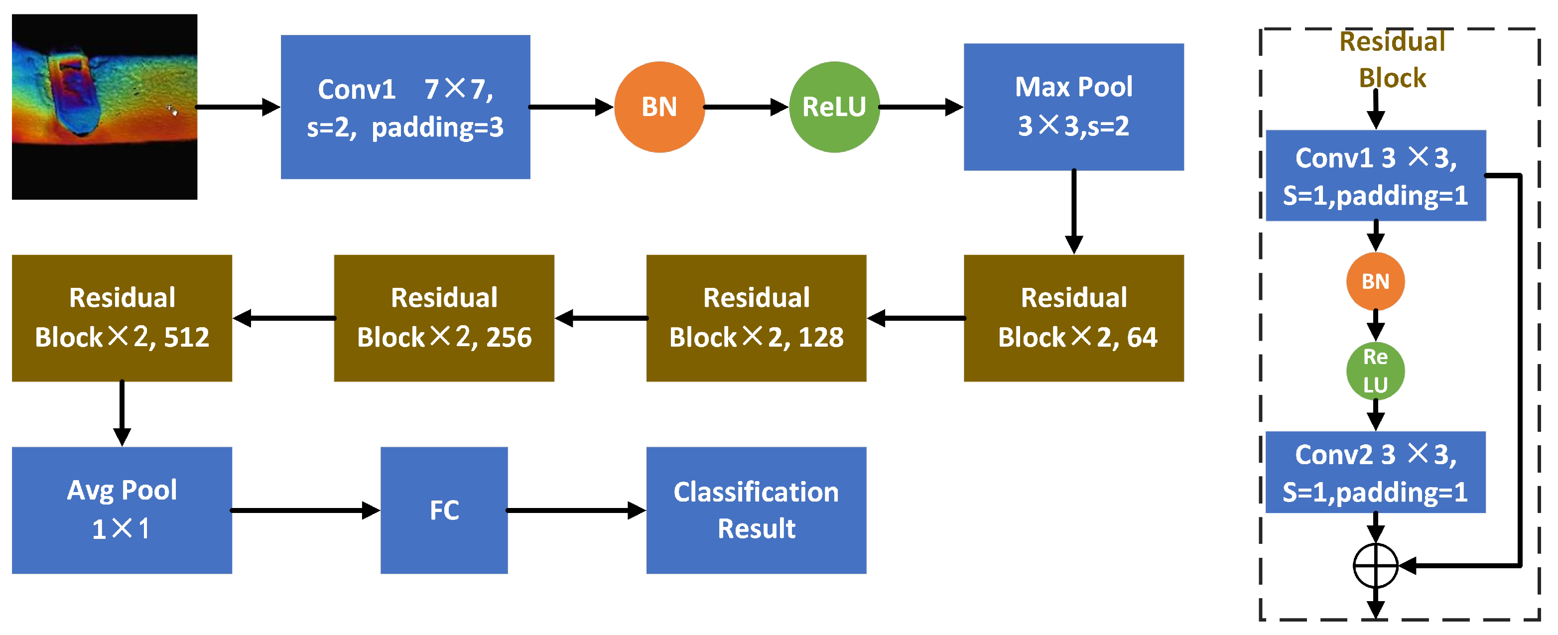
20]. As shown in
Figure 3, the beginning module of ResNet contains a 7 × 7 large convolution kernel and a maximum pooling layer, while the final module contains an average pooling layer and a fully connected layer. ResNets with different depths have the same beginning and final module, and their difference is embodied in the structure and stacking number of residual blocks in the middle layers. The residual block of shallow ResNet models contains two 3 × 3 convolution kernels, two batch normalization (BN) layers, and an activation function (AF). We build the baseline model with two residual blocks stacked in each of the middle four layers, and the input channel dimensions are [64, 128, 256, 1024], from shallow to deep.
2.2.2. The Optimization on ResNet-ACW
To achieve higher accuracy on the sonar image dataset, we modified the baseline model as follows:
- 1
ResNet-18 uses the ReLU function with the formula as follows.
Assume that the input of a neuron is
, the output is
z after multiplying with the weight
W, and the output after ReLU is
. By the forward propagation formula and the ReLU activation function definition, we have
For a fixed learning rate
, the weight
W increases as the absolute value
of the gradient increases. When the next forward propagation is performed, if the output
is less than 0, there is an output
of the activation function, then the chain of the derivation rule has
where the gradient of the weight
W is 0 and it will no longer change according to the weight update formula. At this time,
is an outlier for ReLU, causing the ReLU function to be permanently closed and resulting in the death of neurons.
Swish is an improved activation function based on ReLU and its expression and first derivative function are as shown in Equations (
4) and (
5).
Swish activation function is approaching 0 in the negative semi-axis, which can solve the problem of neuron deactivation. On ResNet-ACW, we replace ReLU with Swish.
- 2
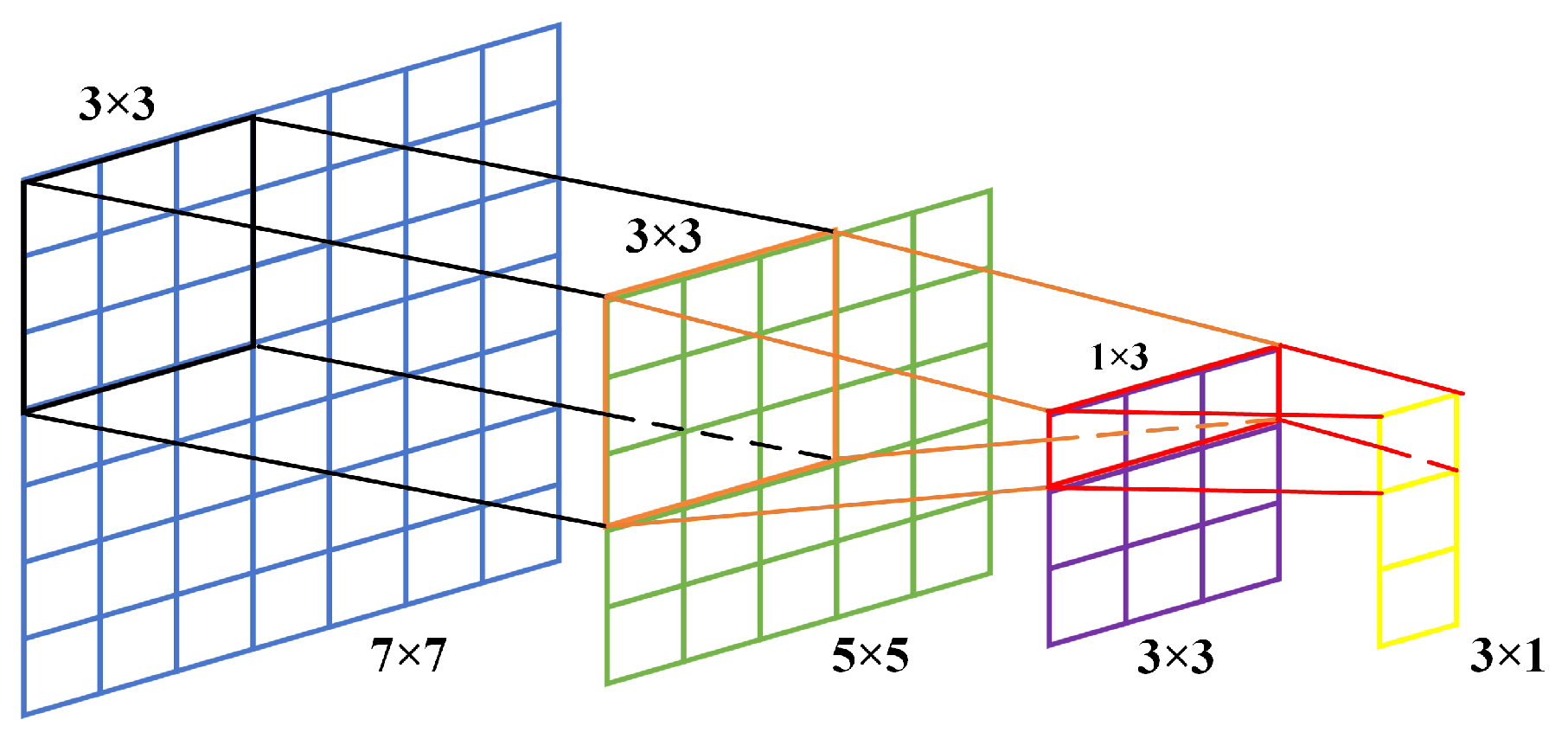
Sonar images have the characteristics of low resolution, low contrast, and blurred object edges. The 7 × 7 convolution kernel used by ResNet-18 is too large to fully abstract its features. Inspired by reference [
21], we decompose the large convolution kernel as shown in
Figure 4. The blue 7 × 7 convolution kernel is decomposed into a black
convolution kernel and a green 5 × 5 convolution kernel. The green 5 × 5 convolution kernel is decomposed into an orange 3 × 3 convolution kernel and purple 3 × 3 convolution kernel. According to the principle of asymmetric convolution [
22], the 3 × 3 convolution kernel is decomposed into smaller red 1 × 3 convolution kernels and yellow 3 × 1 convolution kernels.
We call the first convolutional layer in ResNet-18 as De0, and our proposed convolution kernel decomposition structure as De1 and De2. After decomposition, our structure obtains six convolutional layers with depths [32, 32, 32, 32, 32, 64, 64], deepening the first part of the network with almost constant parameters.
Figure 5 shows the structure of De1 and De2.
- 3
There is redundancy in the residual structure of ResNet-18, which leads to too many similar feature maps generated during the up-dimension operation [
23,
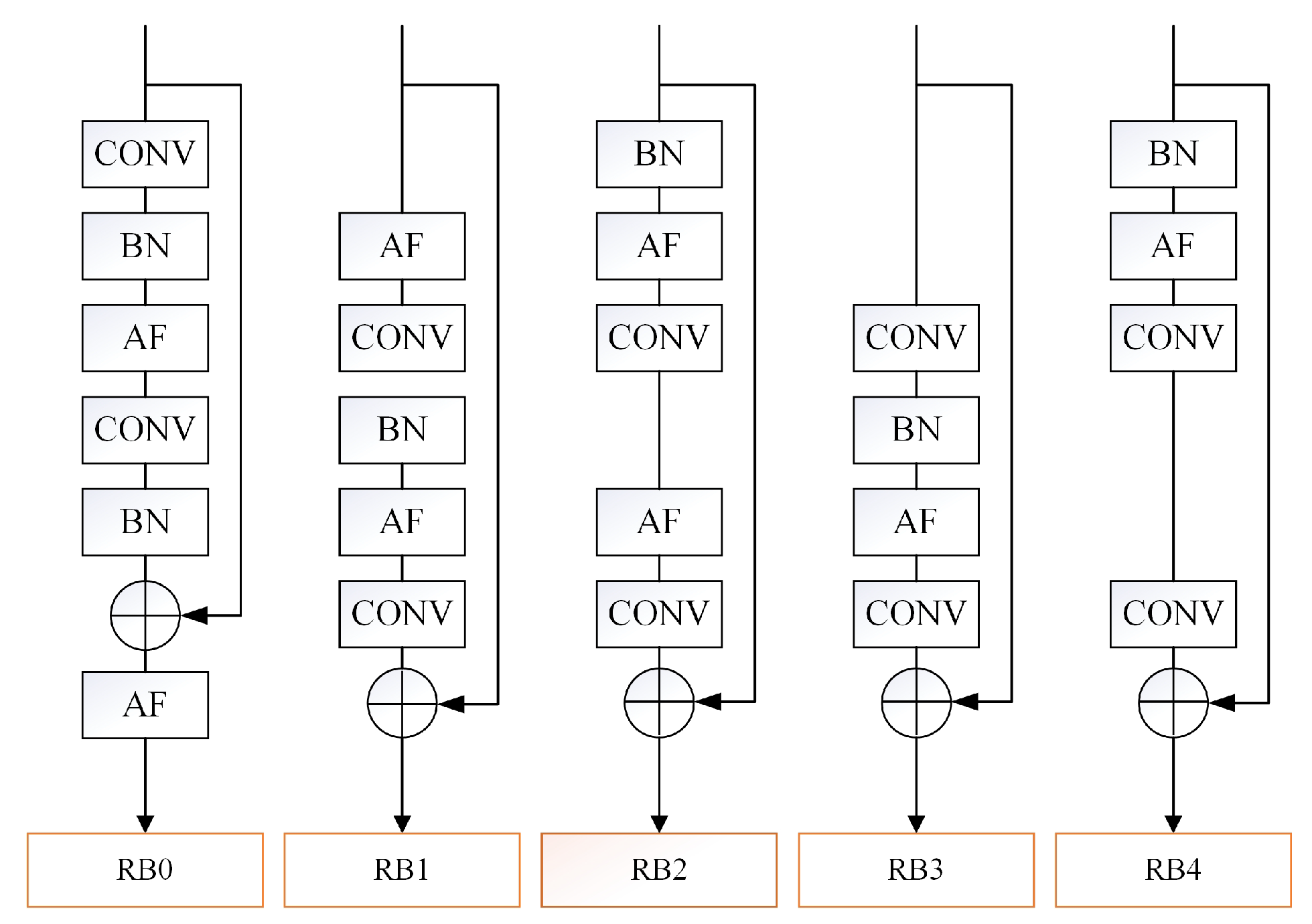
24]. The BN layer performs feature normalization on the entire batch of data and uses the mean and variance of a batch of data to simulate the mean and variance of all data. Due to the small amount of sonar image data and the small batch size, too much use of BN layers in small batch training will make the simulation effect worse and increase the difficulty of network learning. We refer to the residual block structure baseline model as RB0 and the residual block structures proposed in this paper as RB1, RB2, RB3, and RB4, which is shown in
Figure 6. Our proposed RB structures advance the AF layer before CONV to pre-activate CONV and delete a BN layer. RB3 and RB4 have an AF layer reduced on the basis of RB1 and RB2 for comparison.
- 4
Small batch input will also lead to poor stability of network training. Inspired by Dense Connect [
25], this paper proposes a new branch structure: weight reuse structure (WRS). The schematic diagram of the network structure combined with WRS is shown in
Figure 7. WRS reuses the high-order feature matrix output from the last layer of each part of the network. The features are dimensionally reduced and fused by extracting features and downsampling operations again through the convolutional layer on the branch. The depths of the convolution kernels on the three branches are 64, and the sizes of the convolution kernels are [3, 5, 5]. The feature fusion method used in this paper is as follows. After straightening the features of different channels, splice them in sequence, and output them through the fully connected layer. The feature with output of 512 on the trunk is sent to an FC layer with output of 64, and the feature fused in WRS is sent to another. Finally, the outputs of the two FC layers are fused again and sent to the fully connected layer whose output is the number of categories.
2.3. The Proposed GAN
2.3.1. DCGAN
Generative adversarial network is an unsupervised deep learning model. The network model framework consists of generator model and discriminative model. The generator model randomly generates data through certain hidden layer information and the discriminative model estimates whether the sample data come from real training data or the generator model. A common problem when training a GAN is the so-called mode collapse, where the generator produces the same image regardless of the input noise. The DCGAN proposed in 2015 used a convolutional neural network to build the generator and a discriminator, which solved the problems of unstable GAN training, mode collapse, and internal covariate transformation [
26]. Extensive studies have shown that the generator model and discriminative model of DCGAN can learn rich hierarchical representations on object components and backgrounds. Because the GAN proposed in the paper [
26] is designed to generate images with a size of 64 × 64 based on optical images, which is not suitable for the dataset and experimental conditions of our task, we build our GAN based on DCGAN to produce excellent sonar images.
2.3.2. Our Structure (LN-PGAN)
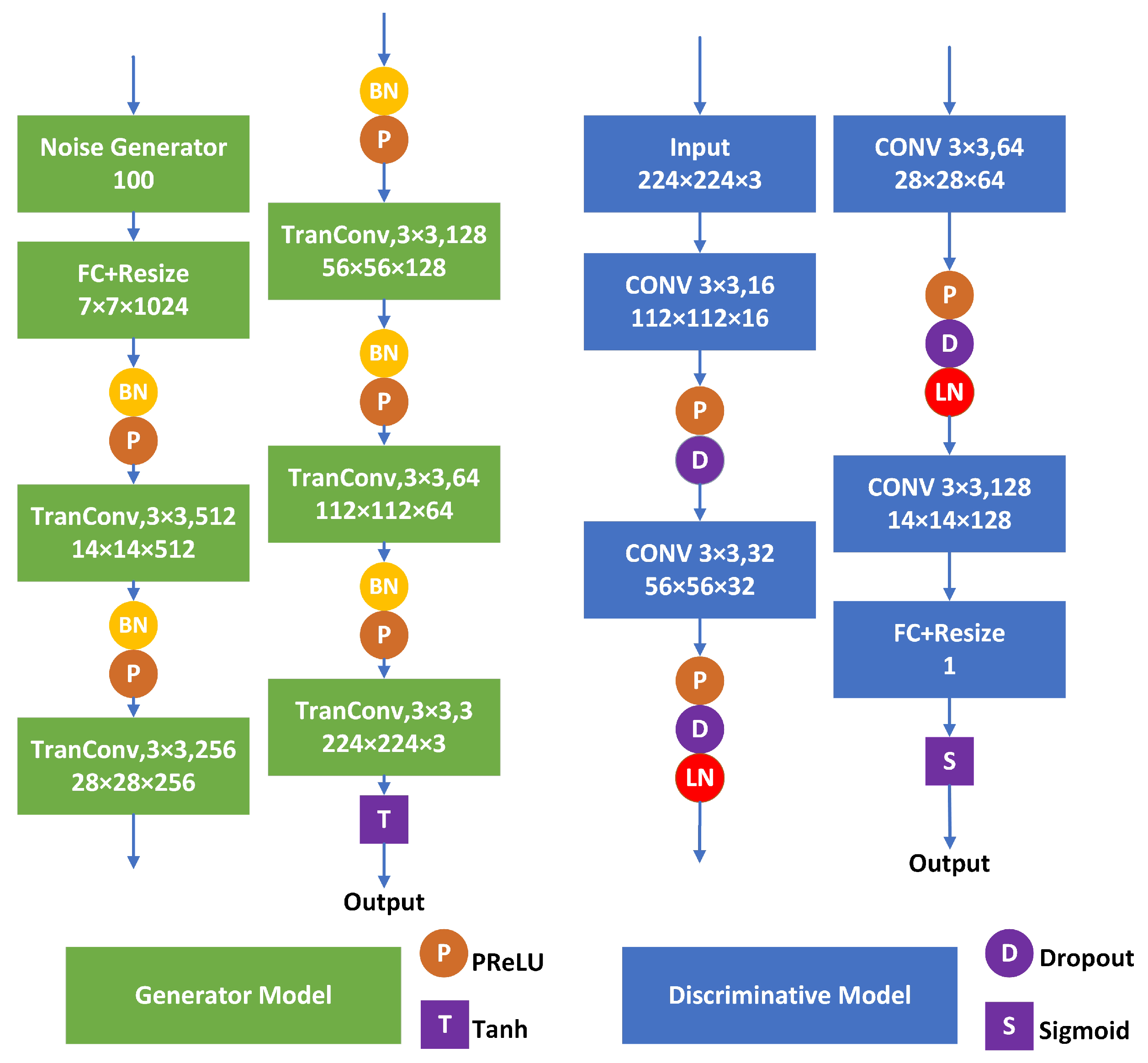
As shown in
Figure 8, the generator model designed in this paper first generates 100-dimensional random noise, maps it to a matrix of size 50,176 through a fully connected layer, and converts it into a matrix of 7 × 7 × 1024. The length and width of the matrix are expanded by the deconvolution operation with a convolution kernel size of 3 × 3 and a stride of 2. Before the deconvolution operation, the eigenvalues are normalized by batch normalization and PReLU activation function to accelerate the convergence of the network and improve the learning ability of the network. After 5 deconvolution layers, the output size is 224 × 224 × 3 generated data. The data generated by the generator model or real data are shuffled and inputted into the discriminative model. In the discriminative model, the image is extracted layer by layer through four convolutional layers with a stride of 2, and a value is output through the fully connected layer. Finally, this value passes through the integrated output discriminative model of the sigmoid activation function to estimate the probability of the source of the image. In the middle of the adjacent convolutional layers, the feature matrix is also integrated to a certain extent through batch normalization and activation function, and at the same time, the drop-out method is used to reduce the overfitting of the network. In particular, in the discriminative model, we replace BN with layer normalization (LN) and use PReLU activation function instead of LeakyReLU in both models. As mentioned earlier, BN normalizes number, weight, and height on the batch, which is not good for small batch size, while LN normalizes channel, weight, and height in channel direction independent of the small batch.
2.3.3. Image Evaluation
In addition to subjective analysis, peak signal-to-noise ratio (PSNR) is generally used to compare the similarity of two images. We can judge the quality of the generated image by GAN through calculating the PSNR of the sample image and the generated image. The PSNR calculation formula of two pictures
I and
K with size
is defined as:
where
is the maximum pixel value of image I, and the mean square error (MSE) is defined as:
In addition, structural similarity (SSIM) is measured from three aspects of lightness
l, contrast
c, and structure
s of two images, which is an effective evaluation index to measure the similarity of images.
where
where
and
are the mean values of
I and
K,
and
are the variances of
I and
K, and
is the covariance of
I and
K. The larger the value of PSNR, the more similar the two pictures are. In addition, the closer the value of SSIM is to 1, the closer the picture generated by the GAN is to the real picture.
2.4. Transfer Learning
Transfer learning applies the knowledge of the source domain and the learning task of the source domain to the learning of the prediction function on the target domain. Fine-tune is a method of transfer learning. This method freezes some layers of the pretrained model, usually the first few convolution layers of the network. The parameters in the frozen layers will not change with training, so it is beneficial to the extraction of the underlying features of the image. Other unfrozen layers of the network are subsequently trained, maintaining some variability in the network. Mini-ImageNet is a sub-dataset of ImageNet, with a total of 100 categories of data and 600 images per category. We pretrain and fine-tune our network model on mini-ImageNet to solve the problems of insufficient network training and low weight utilization.
2.5. The Fusion Few-Shot Strategy
In the methods mentioned in the previous sections, we improved ResNet-18 as a classifier, built a generative adversarial network to expand the dataset, and used the fine-tuning method in transfer learning to initialize and pretrain the network parameters. This section combines the optimization strategies above and proposes a small-sample sonar image classification method that combines multiple optimization strategies.
Figure 9 presents a schematic diagram of the strategy proposed in this paper. The specific steps are as follow:
Divide the dataset into training set, validation set, and testing set;
Input real data into LN-PGAN, generate synthetic data through the training of generative adversarial network, and expand the training set in the dataset according to certain principles;
Perform data preprocessing operations, such as noise reduction and data augmentation, with the training set composed of real data and synthetic data, as the training data of the network;
Based on transfer learning, the network model parameters pretrained with a large amount of data are imported into ResNet-ACW in a fine-tuning method;
Training and classification of ResNet-ACW.
3. Results
We run our model on a desktop workstation with an AMD Ryzen 9 3900X CPU, a 3080 GPU, 64 G of RAM, and Windows 10 as the operating system. To ensure credibility, each classification accuracy result is averaged over five tests.
3.1. Performance Comparison of Classical Networks on Sonar Image Datasets
We build AlexNet, VGG, and ResNet with different layers to compare their performance on our dataset and calculate the parameters and floating-point operations (FLOPs) of each network. For a convolution kernel with a size of
, the general calculation method of the network parameters is as follows:
where
and
are the depths of the input and output feature matrices. The calculation method of the floating-point operand of the general convolutional layer is as follows:
where
and
are the height and width of the output feature matrix of the layer. The FLOPs calculation of the fully connected layer is as follows:
where
I and
O are the number of input and output neurons in the fully connected layer.
Table 2 shows the network parameters, FLOPs, the average accuracy of the test set of five experiments on the sonar image dataset, and the running time of a single experiment for the three classic networks of AlexNet, VGG, ResNet, and their variants. Compared with VGG, ResNet takes up less computing resources and computing time to obtain the best classification results, which is consistent with the results of reference [
11].
3.2. Results of Different Optimization on ResNet-ACW
3.2.1. Activation Function
We replace the ReLU activation function used in the baseline model with a different activation function, including ELU, Swish, and PReLU.
Table 3 shows the test results. The Swish activation function achieves the best performance when applied to the baseline model, while the ELU activation function performs the worst. As a result, we choose Swish as the activation function to optimize the model.
3.2.2. Convolution Kernel Decomposition
We propose two convolution kernel decomposition structures in
Figure 5, named De1 and De2, respectively. In order to verify the improvement effect in the decomposition structure proposed in this paper on the network performance, the first part De0 of the benchmark network is decomposed according to both decomposition structures, and the training is carried out under the same experimental environment and standard. The results are shown in
Table 4, and both of our proposed decomposition structures improve the test accuracy of the baseline model without increasing the amount of parameters and FLOPs. The number of channels for a feature extraction increases with the number of convolution kernels and the network can extract more detailed information, which improves the classification accuracy of the network. Compared with the large convolution kernel, the stacked structure of small convolution kernels increases the number of convolution kernels with the same receptive field. The increase in the number of channels for a feature extraction improves the accuracy of the network, but the number of parameters does not change significantly, which is an advantage brought by the decomposition of large convolution kernels into small convolution kernel structures. Multiple memory calls become more time-consuming, so the decomposition structure will increase the operation time of the network to a certain extent. However, the time cost increase is within an acceptable range and will be resolved with the improvement in the computer hardware.
3.2.3. Residual Block
We propose four residual block structures in
Figure 6, named RB1, RB2, RB3, and RB4, respectively. We train the networks with different residual block structures according to the same experimental environment and standard, and the results are summarized in
Table 5. Changing the structure of the residual block does not affect the number of parameters and FLOPs of the network.
Although the network parameters and complexity of several residual structures are the same, it can be seen from
Table 5 that the pre-activation structure increases the training time of the network. When the convolutional layer is at the top of the structure, the data can be dimensionally reduced, and the latter structure will process the dimensionally reduced data faster. RB2 and RB3, as the improved structure of the residual block optimization in this paper, have achieved good results on the baseline model, among which the structure of RB3 is better. As a comparison structure of RB1, RB3 performs worse than RB0, which shows the importance of pre-activation from the side. In addition, RB4, as the contrast structure of RB2, performs better than RB3 and basically the same as RB0. The result of combining RB2 is better than RB1, which shows that the effect of the BN layer before the first convolutional layer is better than that after the first convolutional layer. To sum up, it is concluded that the residual structure is improved when optimizing the network structure in the sonar image dataset in this paper:
- 1
The pre-activated structure can increase the feature extraction ability of the structure to the input feature matrix, thereby improving the recognition rate of the entire network, but at the same time, it will increase the network running time to a certain extent. It is better not to delete the AF layer easily, which may make the network learn less important complex nonlinear features.
- 2
For sonar image datasets with a small number of samples and a small batch size, a certain BN layer can be deleted, which can effectively improve the accuracy of the network. The BN layer is better placed in the first volume before the accumulation layer, and the normalization of the batch features in advance is conducive to the feature extraction of the subsequent convolutional layers.
3.2.4. Weight Reuse Structure
In the previous discussion, we analyzed the advantages and disadvantages of large convolution kernels and small convolution kernels. Because the small convolution kernels can re-extract the front-end detailed features, and the large convolution kernels can sort out the back-end high-order features, the size selection of the convolution kernels on different branches should follow the principle of keeping the same or increasing from front to back in the WRS. As shown in
Figure 6, we refer to the convolutional layers on the first, second, and third branches as convolutional layer A, convolutional layer B, and convolutional layer C, respectively. In order to choose an optimal structure, the recognition performance when the convolutional layers A, B, and C on the WRS branch are composed of convolution kernels of different sizes is summarized in
Table 6. Convolutional layers A, B, and C are all composed of square convolution kernels with a depth of 64. In the table, ‘1’, ‘3’, and ‘5’ represent the side lengths of the square convolution kernels that make up the convolutional layers. From the results, it can be seen that when A is 3, B is 5, and C is 5, the WRS has the best performance, and when A is 3, B is 3, and C is 3, the performance is worse, which verifies the previous discussion on the role of convolution kernels with different sizes. Therefore, we choose A as 3, B as 5, and C as 5 as the optimal choice of the WRS in this paper.
3.2.5. Combination of the Optimized Structure of the Network
In the previous section, we discussed several structural improvement methods and gave the conclusion of the network structure improvement under the sonar image dataset in this paper. However, these conclusions are based on changes made to the baseline shallow residual network, and the combination of several improved structures has not been discussed. Therefore, it is impossible to determine which combination of structures can obtain the best training and classification results on the sonar image dataset. In order to obtain an optimal result, we combine different activation functions (PReLU, ELU, and Swish), different decomposition structures (De1 and De2), and different residual structure optimizations (RB1 and RB2), respectively, and conduct the training experiments. The results are shown in
Table 7.
There are certain rules through comparison. As we discussed earlier, the Swish function achieves the best performance among all the activation functions and the combination of the ELU function performs the worst. The performance of the decomposition structure De2 is significantly better than that of De1 and the combination of RB2 achieves better results. ResNet-18+Swish+De2+RB2 achieves the best result of 86.27%, which is 4.53% higher than the average accuracy of the baseline model. Through the permutation and combination of several structure optimizations, we obtain two network structure optimization combinations with the best accuracy. Then, these two structural optimization combinations are combined with the WRS again. We call the combination of swish+De1+RB2+WRS as S1 and the combination of swish+De2+RB2+WRS as S2. We also map this structural optimization method to other deep ResNets, and
Table 8 shows the training results. We name the optimal combination ResNet-18+Swish+De2+RB2+WRS as ResNet-ACW. The test results show that our optimization method is effective for residual networks of different depths.
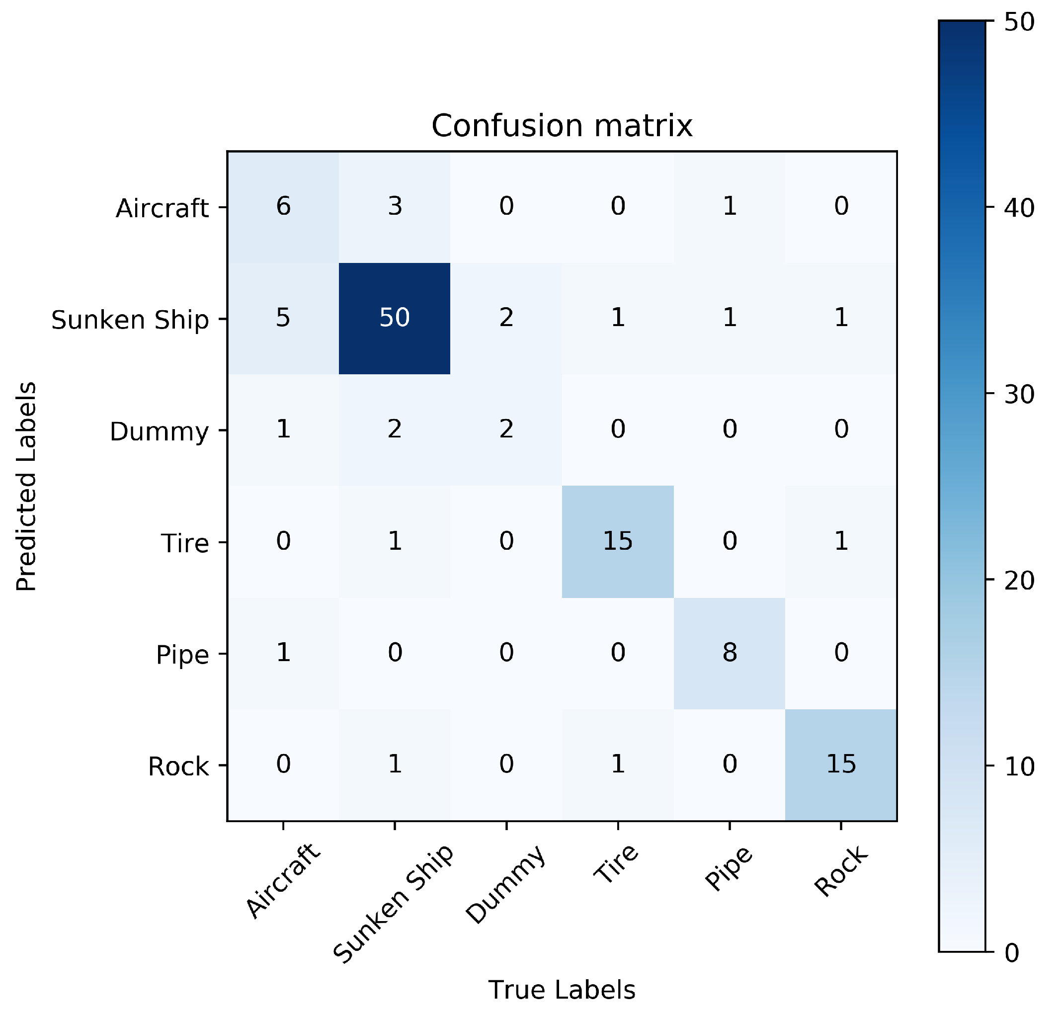
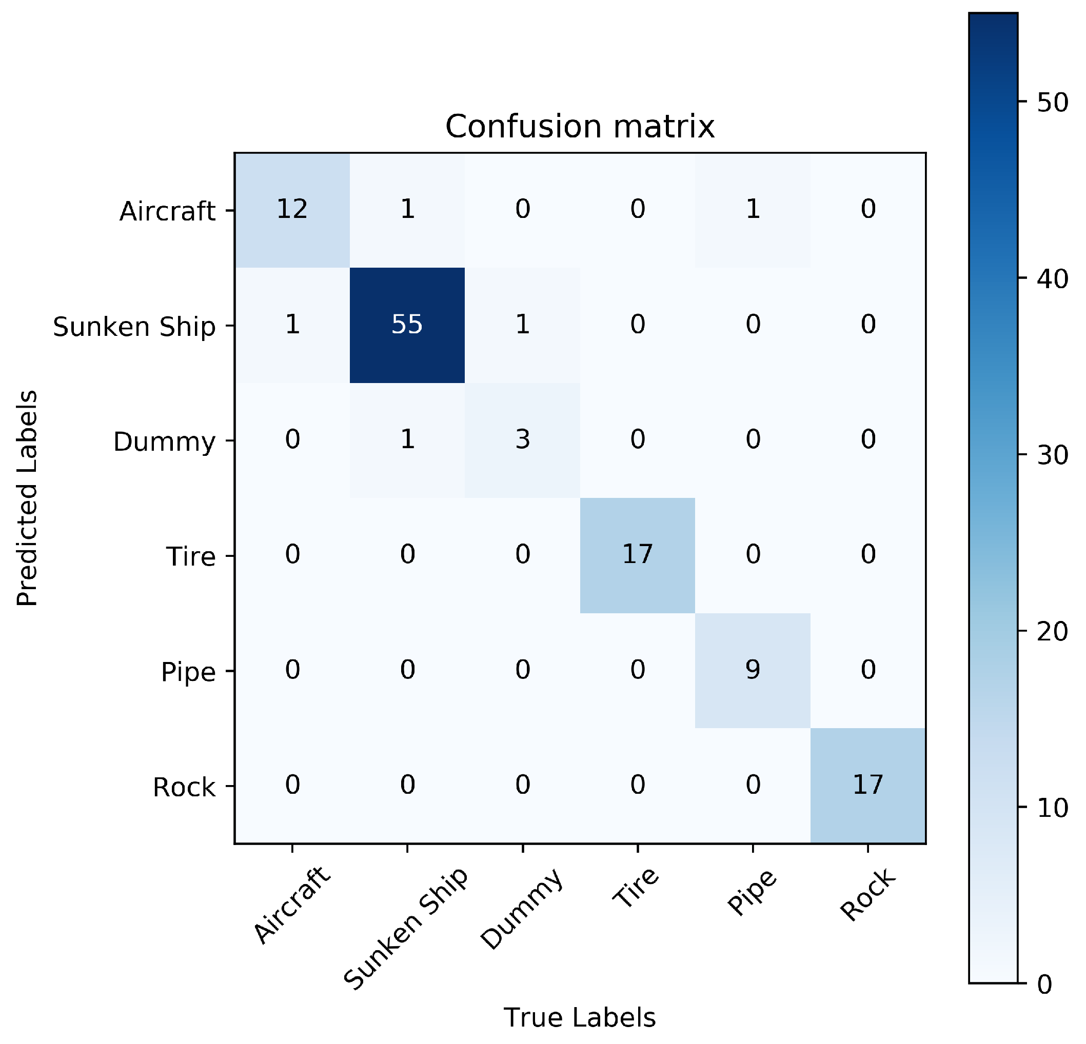
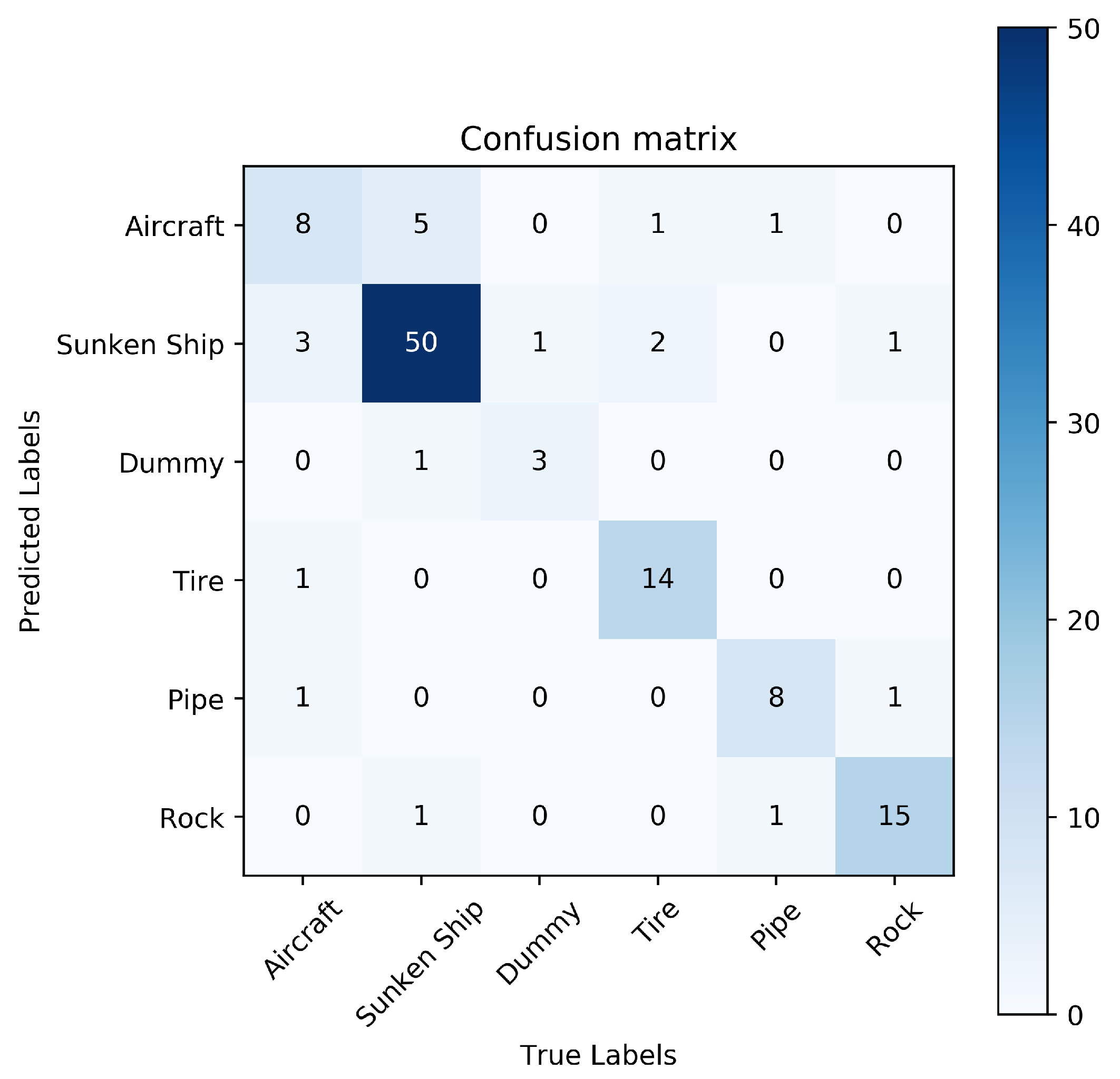
Figure 10 shows the confusion matrix of ResNet-18, and
Figure 11 shows the confusion matrix of ResNet-ACW. By comparing the confusion matrices, we find that the confusion between the aircraft and the sunken ship is severe when classifying with ResNet-18 and our method effectively improves the problem. At the same time, we find that the error rate of the aircraft and dummy is higher, which may be due to the small number of their samples and the failure of the network to better learn their characteristics. Therefore, we need an effective few-shot strategy to solve the above problem.
3.3. LN-P-GAN
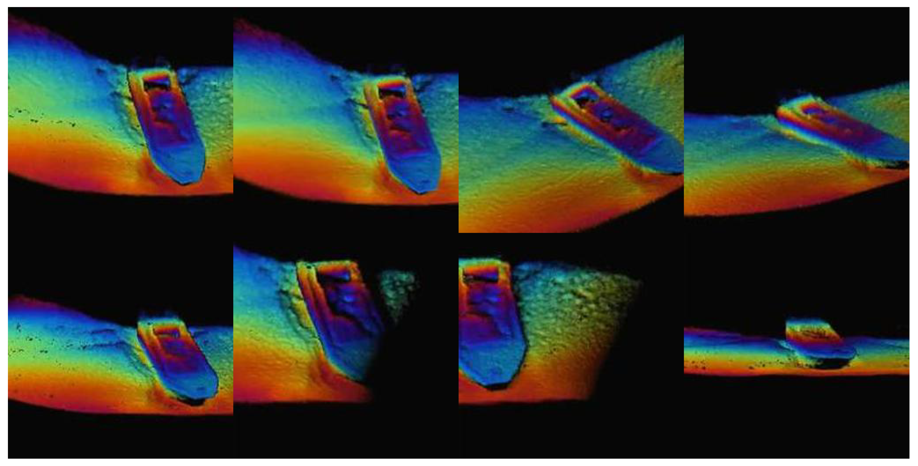
According to the working principle of a GAN, we select several similar sonar images in a class as real data, and then we can generate images that are similar but not identical to real data through the GAN. The generated image has the structural features of the original image and is different from the original image to a certain extent, and the generated image is called synthetic data. Taking the shipwreck sonar image as an example, we input the eight pictures shown in
Figure 12 into the LN-P-GAN constructed in this paper and record the pictures output by the generator model after every 100 iterations.
Figure 13 shows the sonar image of the sunken ship generated by the generator after 5000 iterations. From the given example, it can be seen that the pictures generated by the generator model start with random noise, gradually learn the contour information of the sonar image, reduce the noise, and finally learn more contours. For additional detailed information, it is very close to the real sonar image, but at the same time it incorporates some other real data features, so it is not exactly the same as the original image.
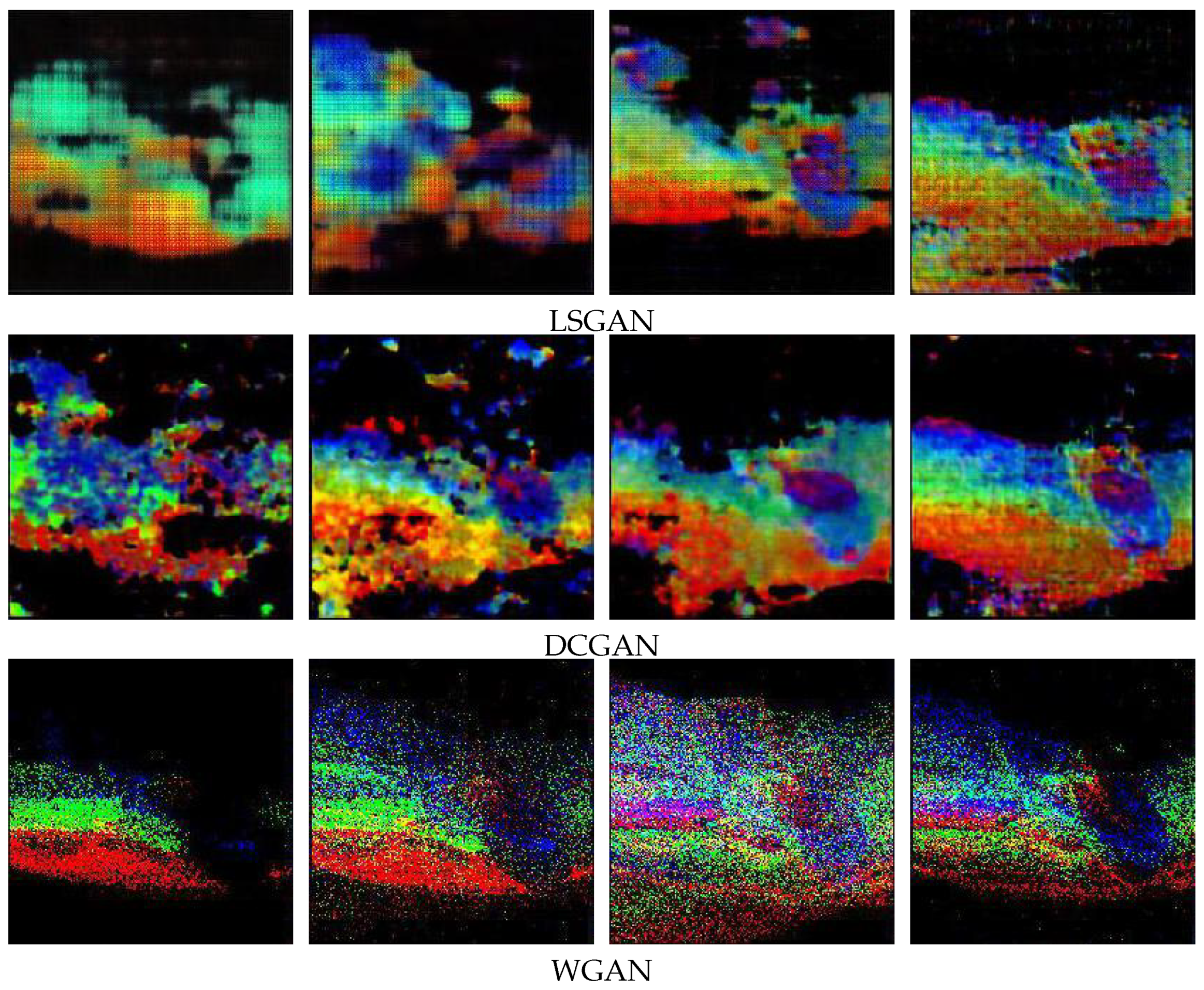
We also build the DCGAN [
26], LSGAN [
27], and WGAN [
28] for the comparison, and the results of the 500th, 1000th, 2000th, and 5000th iterations are shown in
Figure 14. Take 10 pictures generated by four different GANs after 5000 iterations, calculate the PSNR and SSIM with real input pictures according to Equations (
6) and (
10), and take their average values. The results are summarized in
Table 9, and the images generated by the LN-PGAN are better than those generated by the DCGAN, LSGAN, and WGAN in terms of the PSNR and SSIM.
Compared with the DCGAN and LSGAN, the LN-PGAN generates less image noise and converges faster, which proves the effectiveness in optimizing the generator model and the discriminative model. By observing the generated images, we find that the DCGAN and LSGAN do not learn the main features of the source image, which leads to the poor overall retention of the generated images. Although the WGAN has the fastest convergence speed, it has too much noise in the image and lost a lot of information of the source image to generate a usable sonar image. The images generated by the LN-PGAN obtain the highest PSNR and SSIM, which are 20.09 dB and 0.46, respectively, far higher than other GANs. The higher PSNR and SSIM prove that our image is closer to the real sonar image. At the same time, the value of the SSIM is 0.46, which shows that the image we generate is still different from the source image, supplementing the feature breadth of network learning and avoiding the problems in [
19].
We expand the samples according to the classification accuracy of the network and test the baseline network and ResNet-ACW on the expanded dataset.
Table 10 shows that ResNet ACW achieves 93.77% accuracy by reasonably expanding the dataset with the synthetic data generated by the GAN. It is an effective and practical method to enlarge the data regularly through the GAN, which reduces the overfitting of the network and solves the problem of insufficient underwater sonar image data. It can be predicted that continuing to expand the dataset can still reduce the network overfitting to a certain extent, but it also needs to pay the cost of increased training time.
3.4. Transfer Learning
We use the same method as in this paper to partition the mini-ImageNet dataset and then pretrain and fine-tune our model on the partitioned data. For ResNet, the first five sections are available for freezing. We call the number of frozen parts
.
represents that the first five parts are frozen, and
means that network parameters are not frozen.
Table 11 shows the fine-tuning test results of the baseline model and ResNet-ACW. As can be seen from the results in
Table 11, the fine-tuning method can greatly improve the accuracy of the network verification set, indicating that the network parameters pretrained by Mini-ImageNet are successfully transferred to the network used for sonar image recognition. When
, both the baseline and ResNet-ACW achieve the best network recognition rate.
3.5. The Fusion Strategy
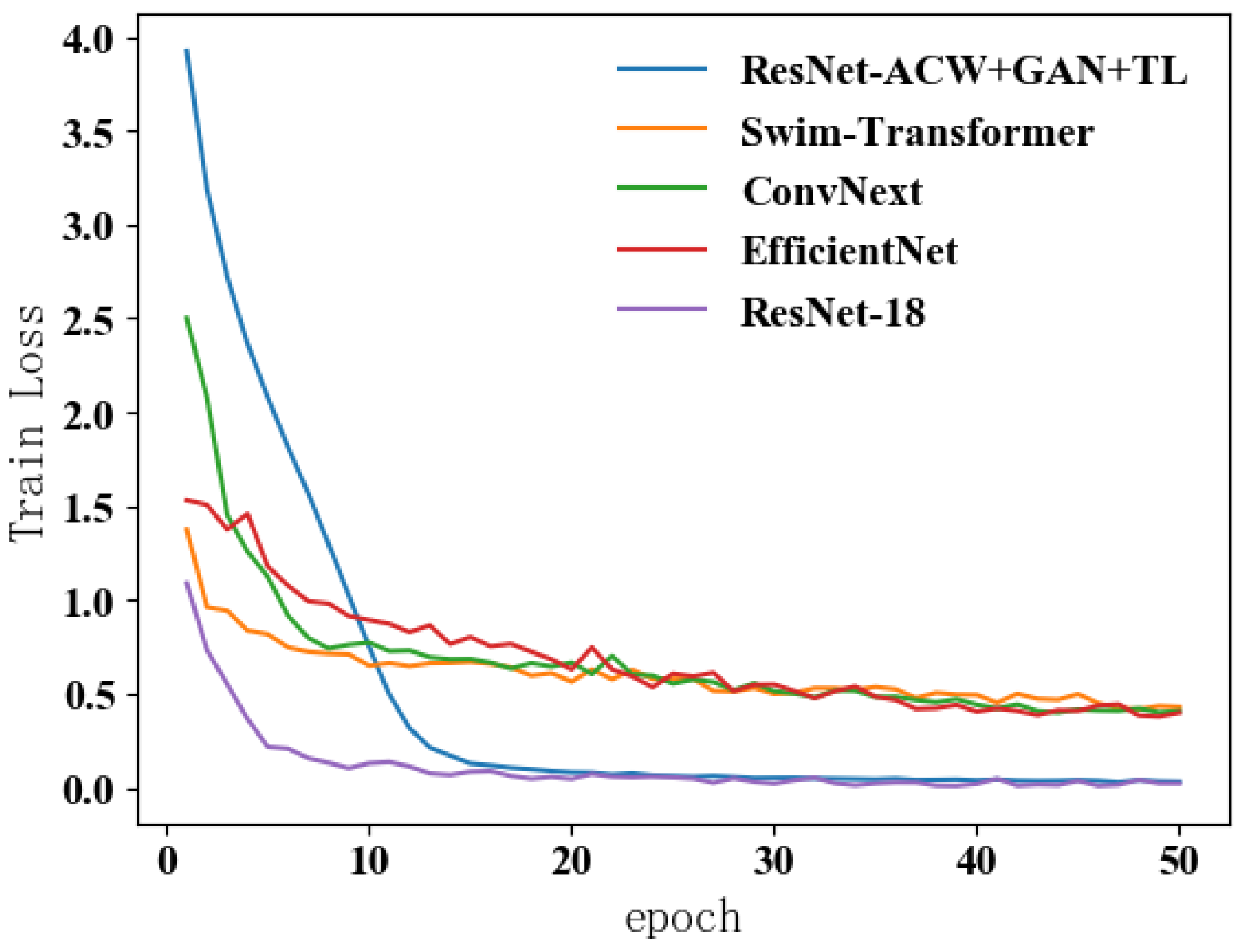
We combine each optimization part proposed in this paper according to the process shown in
Figure 9 and compare the training process optimized by this combination strategy with some novel used network structures, such as EfficientNet [
29], Convnext [
30], and SwinTransformer [
31].
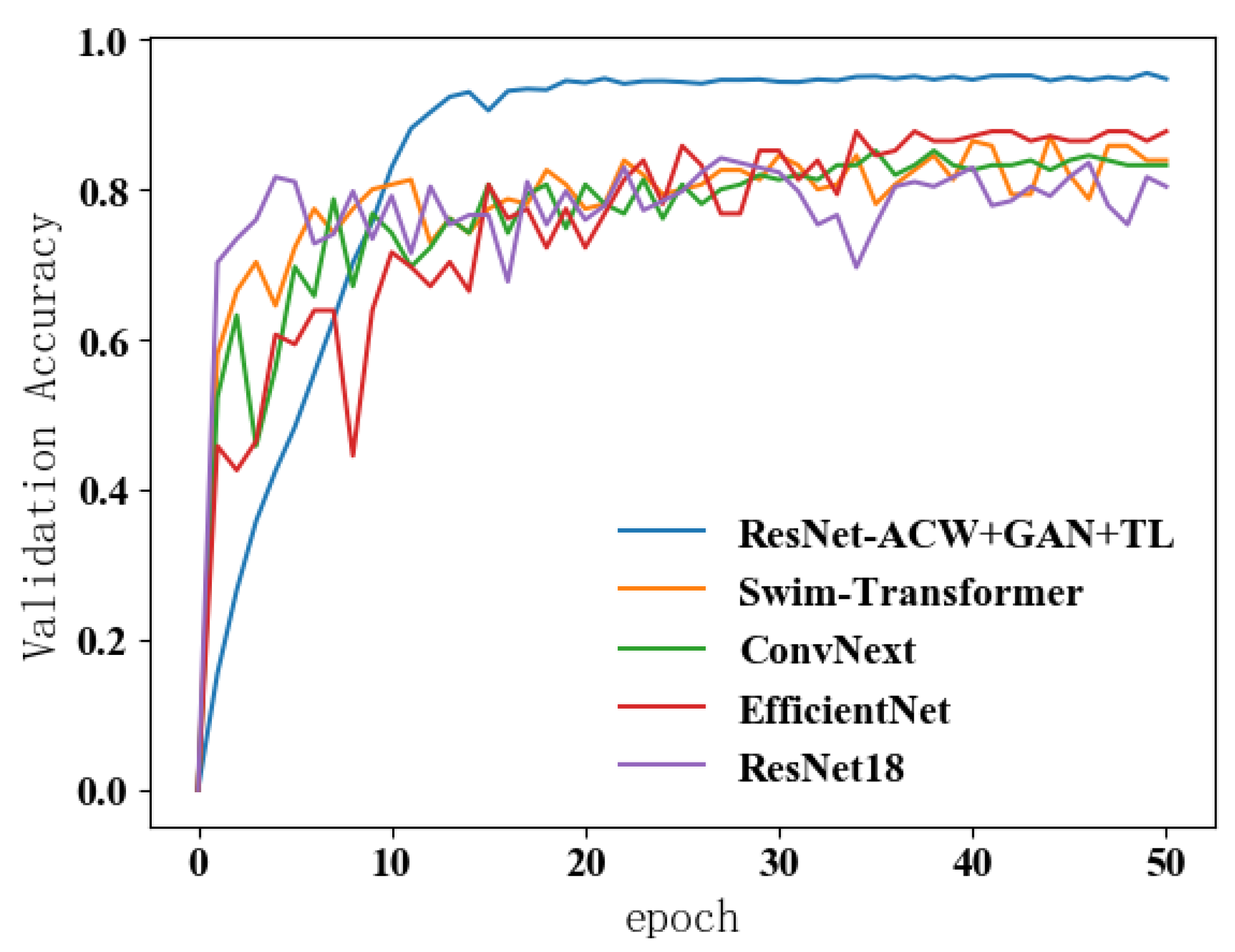
Figure 15 shows the validation accuracy curves of these networks, and
Figure 16 shows their training losses.
Table 12 shows the test accuracy of these networks and our method. Finally, ResNet-ACW using the fusion strategy achieves the optimal test set classification accuracy of 95.93% and improves by about 15% compared with the baseline model. It can be seen from the training results that contrast to the state-of-the-art networks or transformer models, the training process of our method is more stable and converges faster.
Figure 17,
Figure 18,
Figure 19 and
Figure 20 show the confusion matrices of ResNet-ACW+GAN+FL, SwinTransformer, ConvNext, and EfficientNet, respectively. Compared with
Figure 11, our method significantly improves the discrimination of confusing aircrafts and sunken ships and improves the overall classification accuracy. Observing the state-of-the-art classification models, we find that although these models are better than the ResNet-18 classification, they still fail to solve the accurate classification of confusing items. Our proposed network model outperforms these models without the optimization of the few-shot fusion strategies. After the GAN and FL, our method has no obvious confusion, and the classification accuracy is much higher than these methods. The result verifies the reliability of our method.
4. Conclusions and Discussion
This work has contributed to the classification task of sonar images. We have built a sonar image dataset of 768 images with RGB and single-channel data which contains six categories of targets. By comparing the common sonar image classifiers such as AlexNet, VGG, and ResNet, we found that ResNet-18 performs best on our dataset. In order to better classify the sonar images, we improved ResNet-18 around four aspects, the activation function, convolution kernel decomposition, residual block, and weight reuse structure, and propose our new network model ResNet-ACW. The improvements based on the activation function and the residual block did not increase the parameters, FLOPs, and calculation time of the network but achieved better classification results. The convolution kernel decomposition structure increased the number of FLOPs and a few parameters and increased the classification accuracy at the expense of a certain calculation time. The increased weight reuse structure could make the training process of the network more stable and improve the ability of the network to extract image features. The proposed ResNet-ACW achieved 87.01% accuracy, which was 5.27% higher than ResNet-18 and even exceeded the state-of-the-art classifier models. By analyzing the confusion matrices, we found that although ResNet-ACW improved the accuracy, there were still confusion terms, which is caused by the insufficient learning of the sonar image features. Therefore, we need to optimize the few-shot strategy for the classification process.
We proposed a fusion few-shot strategy based on a GAN and transfer learning. The fusion strategy consists of a novel GAN (LN-PGAN) and a fine-tuning method in transfer learning. We improved the generator model and discriminative model and proposed the LN-PGAN based on the DCGAN. By comparing with the DCGAN, WGAN, and LSGAN, our GAN model achieved a higher PSNR and SSIM, which means the synthetic image is closer to real sonar image data. At the same time, the synthetic data generated by the LN-PGAN were different from the source image with sonar image features, which provided additional features for the network to learn. We used the fine-tuning method in transfer learning to pretrain the network and obtained the best effect by freezing different layers. The fine-tuning method improved the ability of the network convolution kernel to extract features by freezing the training of the network parameters layer by layer, which reduced the parameters of the network and finally effectively reduced the overfitting. After the fusion optimization, our method achieves 95.93% classification accuracy on the sonar image dataset. Through the training and loss curves, our method avoided the overfitting problem and the low accuracy problem under small samples. Meanwhile, our algorithm had a faster fitting speed and a more stable training process to make the algorithm more robust. According to the confusion matrices, our algorithm overcame the classification problem of confusing items and could accurately extract the key features between the different categories.
Restricted to the sonar image collecting way, however, the types of datasets we built were not complex, both with a data imbalance problem. In the following work, we will continue to supplement our sonar image data, including some closer targets formed in worse environments, and further study the training problems caused by the sample imbalance. We observed shadows in some sonar images and the shadows are often close to the target itself. It is difficult to remove the shadow by a method such as saliency segmentation and directly find that the feature block in the image comes from which part of the original image in the deep feature map extracted by the network. Meanwhile, some sonar images often provide additional information, such as backscatter maps, when they are formed. How to input them into the network as a priori knowledge will also be our follow-up work.
In summary, we built a new network model ResNet-ACW for sonar image datasets, which works well on both RGB and single-channel image data. Aiming at the overfitting problem and low classification accuracy of a deep learning model under small samples, we propose a new generative adversarial network and combine it with the fine-tuning method in transfer learning. The results show that the network structure optimization method based on sonar images and the training optimization scheme based on the fusion strategy can effectively improve the sonar image classification accuracy and reduce the overfitting of a network. Our algorithm achieves a classification accuracy of 95.93% on the six-category target sonar image dataset, which is 14.19% higher than the baseline model.
Author Contributions
Conceptualization, Z.D.; methodology, Z.D.; software, Z.D.; validation, Z.D., H.L. and T.D.; formal analysis, Z.D.; investigation, Z.D. and T.D.; data curation, Z.D.; writing—original draft preparation, Z.D.; writing—review and editing, H.L. and T.D.; supervision, H.L.; project administration, H.L.; funding acquisition, H.L. All authors have read and agreed to the published version of the manuscript.
Funding
This research was funded by the National Natural Science Foundation of China under grant number 61971354.
Institutional Review Board Statement
Not applicable.
Informed Consent Statement
Not applicable.
Data Availability Statement
Not applicable.
Conflicts of Interest
The authors declare no conflict of interest.
References
- Radeta, M.; Zuniga, A.; Motlagh, N.H.; Liyanage, M.; Freitas, R.; Youssef, M.; Nurmi, P. Deep Learning and the Oceans. Computer 2022, 55, 39–50. [Google Scholar] [CrossRef]
- Xu, H.; Yang, L.; Long, X. Underwater Sonar Image Classification with Small Samples Based on Parameter-based Transfer Learning and Deep Learning. In Proceedings of the 2022 Global Conference on Robotics, Artificial Intelligence and Information Technology (GCRAIT), Chicago, IL, USA, 30–31 July 2022. [Google Scholar]
- Krishnan, H.; Lakshmi, A.A.; Anamika, L.S.; Athira, C.H.; Alaikha, P.V.; Manikandan, V.M. A Novel Underwater Image Enhancement Technique using ResNet. In Proceedings of the 2020 IEEE 4th Conference on Information & Communication Technology (CICT), Chennai, India, 3–5 December 2020; pp. 1–5. [Google Scholar]
- Nguyen, H.-T.; Eon-Ho, L.; Sejin, L. Study on the Classification Performance of Underwater Sonar Image Classification Based on Convolutional Neural Networks for Detecting a Submerged Human Body. Sensors 2020, 20, 94. [Google Scholar] [CrossRef] [PubMed]
- Liu, F.; Ding, H.; Li, D.; Wang, T.; Luo, Z.; Chen, L. Few-shot Learning with Data Enhancement and Transfer Learning for Underwater Target Recognition. In Proceedings of the 2021 OES China Ocean Acoustics (COA), Harbin, China, 14–17 July 2021. [Google Scholar]
- Lecun, Y.; Bengio, Y.; Hinton, G. Deep learning. Nature 2015, 521, 436–444. [Google Scholar] [CrossRef] [PubMed]
- Neupane, D.; Seok, J. Bearing fault detection and diagnosis using case Western Reserve University dataset with deep learning approaches: A review. IEEE Access 2020, 8, 93155–93178. [Google Scholar] [CrossRef]
- Seok, J. Active sonar target classification using multi-aspect sensing and deep belief networks. Int. J. Eng. Res. Technol. 2018, 11, 1999–2008. [Google Scholar]
- Wu, M.; Wang, Q.; Rigall, E.; Li, K.; Zhu, W.; He, B.; Yan, T. ECNet: Efficient convolutional networks for side scan sonar image segmentation. Sensors 2019, 19, 2009. [Google Scholar] [CrossRef] [PubMed]
- Li, C.; Huang, Z.; Xu, J.; Guo, X.; Gong, Z.; Yan, Y. Multi-channel underwater target recognition using deep learning. Acta Acust. 2020, 45, 506–514. [Google Scholar]
- Qin, X.; Luo, X.; Wu, Z.; Shang, J. Optimizing the Sediment Classification of Small Side-Scan Sonar Images Based on Deep Learning. IEEE Access 2021, 9, 29416–29428. [Google Scholar] [CrossRef]
- Jin, L.; Liang, H.; Yang, C. Sonar image recognition of underwater target based on convolutional neural network. J. Northwestern Polytech. Univ. 2021, 39, 285–291. [Google Scholar] [CrossRef]
- Li, C.; Ye, X.; Cao, D.; Hou, J.; Yang, H. Zero shot objects classification method of side scan sonar image based on synthesis of pseudo samples. Appl. Acoust. 2021, 173, 107691. [Google Scholar] [CrossRef]
- Huang, C.; Zhao, J.; Yu, Y.; Zhang, H. Comprehensive Sample Augmentation by Fully Considering SSS Imaging Mechanism and Environment for Shipwreck Detection Under Zero Real Samples. IEEE Trans. Geosci. Remote Sens. 2022, 60, 1–14. [Google Scholar] [CrossRef]
- Zhou, Y.; Chen, S.-C.; Wu, K.; Ning, M.-Q.; Chen, H.-K.; Zhang, P. SCTD 1.0:Sonar Common Target Detection Dataset. Comput. Sci. 2021, 48, 334–339. [Google Scholar]
- Chen, Y.; Liang, H.; Pang, S. Study on Small Samples Active Sonar Target Recognition Based on Deep Learning. J. Mar. Sci. Eng. 2022, 10, 1144. [Google Scholar] [CrossRef]
- Yulin, T.A.N.G.; Shaohua, J.I.N.; Gang, B.I.A.N.; Yonghou, Z.H.A.N.G.; Fan, L.I. The transfer learning with convolutional neural network method of side-scan sonar to identify wreck images. Acta Geod. Cartogr. Sin. 2021, 50, 260–269. [Google Scholar]
- Huo, G.; Wu, Z.; Li, J. Underwater Object Classification in Sidescan Sonar Images Using Deep Transfer Learning and Semisynthetic Training Data. IEEE Access 2020, 8, 47407–47418. [Google Scholar] [CrossRef]
- Steiniger, Y.; Kraus, D.; Meisen, T. Generating SyntheticSidescan Sonar Snippets Using Transfer-Learning in Generative Adversarial Networks. J. Mar. Sci. Eng. 2021, 9, 239. [Google Scholar] [CrossRef]
- He, K.; Zhang, X.; Ren, S.; Sun, J. Deep Residual Learning for Image Recognition. In Proceedings of the 2016 IEEE Conference on Computer Vision and Pattern Recognition (CVPR), Las Vegas, NV, USA, 27–30 June 2016; pp. 770–778. [Google Scholar]
- Srivastava, N.; Hinton, G.; Krizhevsky, A.; Sutskever, I.; Salakhutdinov, R. Dropout: A simple way to prevent neural networks from overfitting. J. Mach. Learn. Res. 2014, 15, 1929–1958. [Google Scholar]
- Szegedy, C.; Vanhoucke, V.; Ioffe, S.; Shlens, J.; Wojna, Z. Rethinking the Inception Architecture for Computer Vision. In Proceedings of the 2016 IEEE Conference on Computer Vision and Pattern Recognition (CVPR), Las Vegas, NV, USA, 27–30 June 2016; pp. 2818–2826. [Google Scholar]
- Han, K.; Wang, Y.; Tian, Q.; Guo, J.; Xu, C.; Xu, C. GhostNet: More features from cheap operations. In Proceedings of the 2020 IEEE/CVF Conference on Computer Vision and Pattern Recognition (CVPR), Seattle, CA, USA, 27 June–1 July 2020; pp. 1577–1586. [Google Scholar]
- Chu, Y.; Wang, J.; Zhang, X.; Liu, H. Image Classification Algorithm Based on ImprovedDeep Residual Network. J. Univ. Electron. Sci. Technol. China 2021, 50, 243–248. [Google Scholar]
- Huang, G.; Liu, Z.; Van Der Maaten, L.; Weinberger, K.Q. Densely Connected Convolutional Networks. In Proceedings of the 2017 IEEE Conference on Computer Vision and Pattern Recognition (CVPR), Honolulu, HI, USA, 21–26 July 2017; pp. 2261–2269. [Google Scholar]
- Radford, A.; Metz, L.; Chintala, S. Unsupervised Representation Learning with Deep Convolutional Generative Adversarial Networks. arXiv 2015, arXiv:1511.06434. [Google Scholar]
- Qi, G. Loss-Sensitive Generative Adversarial Networks on Lipschitz Densities. Int. J. Comput. Vis. 2020, 128, 1118–1140. [Google Scholar] [CrossRef]
- Arjovsky, M.; Chintala, S.; Bottou, L. Wasserstein GAN. arXiv 2017, arXiv:1701.07875. [Google Scholar]
- Tan, M.; Le, Q. EfficientNet: Rethinking Model Scaling for Convolutional Neural Networks. In Proceedings of the International Conference on Machine Learning (ICML), Long Beach, CA, USA, 10–15 June 2019. [Google Scholar]
- Liu, Z.; Mao, H.; Wu, C.Y.; Feichtenhofer, C.; Darrell, T.; Xie, S. A ConvNet for the 2020s. arXiv 2022, arXiv:2201.03545. [Google Scholar]
- Liu, Z.; Lin, Y.; Cao, Y.; Hu, H.; Wei, Y.; Zhang, Z.; Guo, B. Swin Transformer: Hierarchical Vision Transformer using Shifted Windows. arXiv 2021, arXiv:2103.14030. [Google Scholar]
Figure 1.
The context of this paper.
Figure 1.
The context of this paper.
Figure 2.
Sonar image in the dataset.
Figure 2.
Sonar image in the dataset.
Figure 3.
The structure of ResNet-18.
Figure 3.
The structure of ResNet-18.
Figure 4.
Convolution kernel decomposition.
Figure 4.
Convolution kernel decomposition.
Figure 5.
Structure of De1 and De2.
Figure 5.
Structure of De1 and De2.
Figure 6.
Residual block structures.
Figure 6.
Residual block structures.
Figure 7.
Convolution kernel decomposition.
Figure 7.
Convolution kernel decomposition.
Figure 8.
Flow of LN-PGAN.
Figure 8.
Flow of LN-PGAN.
Figure 9.
Flow of the fusion few-shot strategy.
Figure 9.
Flow of the fusion few-shot strategy.
Figure 10.
Confusion matrix of ResNet-18.
Figure 10.
Confusion matrix of ResNet-18.
Figure 11.
Confusion matrix of ResNet-ACW.
Figure 11.
Confusion matrix of ResNet-ACW.
Figure 12.
LN-P-GAN input image.
Figure 12.
LN-P-GAN input image.
Figure 13.
Output image of LN-PGAN.
Figure 13.
Output image of LN-PGAN.
Figure 14.
Output image of the contrastive GANs.
Figure 14.
Output image of the contrastive GANs.
Figure 15.
Val_acc curves of networks.
Figure 15.
Val_acc curves of networks.
Figure 16.
Train losses of the networks.
Figure 16.
Train losses of the networks.
Figure 17.
ResNet-ACW+GAN+FL.
Figure 17.
ResNet-ACW+GAN+FL.
Figure 18.
SwinTransformer.
Figure 18.
SwinTransformer.
Table 1.
The quantity of samples in each category.
Table 1.
The quantity of samples in each category.
| Category | Aircraft | Sunken Ship | Dummy | Tire | Pipe | Rock | Total |
|---|
| Quantity | 87 | 379 | 28 | 112 | 70 | 110 | 786 |
Table 2.
Performance summary of several classical networks on sonar image datasets.
Table 2.
Performance summary of several classical networks on sonar image datasets.
| Network | Parameters | FLOPs | Test Accuracy | Training Time |
|---|
| AlexNet | 14.60 M | 0.62 G | 74.13% | 1150 s |
| VGG-11 | 64.82 M | 15.12 G | 76.46% | 2703 s |
| VGG-13 | 65.00 M | 22.54 G | 77.65% | 3619 s |
| VGG-16 | 70.31 M | 30.88 G | 77.12% | 4199 s |
| VGG-19 | 75.62 M | 39.20 G | 78.13% | 4795 s |
| ResNet-18 | 11.18 M | 3.64 G | 81.74% | 1583 s |
| ResNet-34 | 21.29 M | 7.36 G | 81.03% | 2027 s |
| ResNet-50 | 25.05 M | 8.24 G | 80.69% | 2886 s |
| ResNet-101 | 44.04 M | 15.70 G | 81.55% | 4097 s |
Table 3.
The quantity of samples in each category.
Table 3.
The quantity of samples in each category.
| Network | Activation Function | Test Accuracy | Accuracy Increment | Training Time |
|---|
| Baseline Model | ReLU | 81.74% | / | 1583 s |
| PReLU | 82.21% | 0.47% | 1649 s |
| ELU | 81.43% | −0.31% | 1596 s |
| Swish | 82.85% | 1.11% | 1787 s |
Table 4.
Test results of the convolution kernel decomposition structure.
Table 4.
Test results of the convolution kernel decomposition structure.
| Network | De Structure | Parameters | FLOPs | Test Accuracy | Accuracy Increment | Training Time |
|---|
| Baseline Model | De0 | 11.18 M | 3.64 G | 81.74% | / | 1583 s |
| De1 | 11.20 M | 4.10 G | 83.82% | 2.08% | 1783 s |
| De2 | 11.20 M | 4.10 G | 83.14% | 1.40% | 1778 s |
Table 5.
Test results of the residual block structure.
Table 5.
Test results of the residual block structure.
| Network | Residual Block | Test Accuracy | Accuracy Increment | Training Time |
|---|
| Baseline Model | RB0 | 81.74% | / | 1583 s |
| RB1 | 83.48% | 1.74% | 1605 s |
| RB2 | 83.81% | 2.07% | 1626 s |
| RB3 | 81.09% | −0.65% | 1590 s |
| RB4 | 81.75% | 0.01% | 1595 s |
Table 6.
Effect of the size of the convolution kernel on the WRS branch.
Table 6.
Effect of the size of the convolution kernel on the WRS branch.
| Network | A | B | C | Test Accuracy | Accuracy Increment |
|---|
| Baseline Model | / | / | / | 81.74% | / |
| ResNet-18+WRS | 1 | 1 | 1 | 83.04% | 1.30% |
| 1 | 1 | 3 | 83.42% | 1.68% |
| 1 | 3 | 3 | 83.63% | 1.89% |
| 1 | 3 | 5 | 84.15% | 2.41% |
| 1 | 5 | 5 | 84.11% | 2.37% |
| 3 | 3 | 3 | 83.17% | 1.43% |
| 3 | 3 | 5 | 84.04% | 2.30% |
| 3 | 5 | 5 | 84.92% | 3.18% |
| 5 | 5 | 5 | 84.63% | 2.89% |
Table 7.
Test results of different structural combinations.
Table 7.
Test results of different structural combinations.
| Network | Activation Function | Decomposition | Residual Block | Test Accuracy | Accuracy Increment |
|---|
| Baseline Model | PReLU | De1 | RB1 | 83.12% | 1.38% |
| De1 | RB2 | 84.13% | 2.43% |
| De2 | RB1 | 84.81% | 3.07% |
| De2 | RB2 | 85.48% | 3.74% |
| ELU | De1 | RB1 | 82.78% | 1.04% |
| De1 | RB2 | 83.18% | 1.44% |
| De2 | RB1 | 83.11% | 1.37% |
| De2 | RB2 | 83.13% | 1.39% |
| Swish | De1 | RB1 | 83.44% | 1.70% |
| De1 | RB2 | 85.82% | 4.08% |
| De2 | RB1 | 85.68% | 3.94% |
| De2 | RB2 | 86.27% | 4.53% |
Table 8.
Test results of S1 and S2 structures combined with ResNet of different depths.
Table 8.
Test results of S1 and S2 structures combined with ResNet of different depths.
| Network | Test Accuracy | Accuracy Increment | Training Time |
|---|
| ResNet-18-S1 | 86.84% | 5.1% | 2327 s |
| ResNet-ACW | 87.01% | 5.27% | 2484 s |
| ResNet-34-S1 | 85.94% | 4.91% | 3143 s |
| ResNet-34-S2 | 86.37% | 5.34% | 3086 s |
| ResNet-50-S1 | 85.72% | 5.03% | 4687 s |
| ResNet-50-S2 | 86.10% | 5.41% | 4312 s |
| ResNet-101-S1 | 86.19% | 4.64% | 6051 s |
| ResNet-101-S2 | 86.38% | 4.83% | 5933 s |
Table 9.
Comparison of the generated images.
Table 9.
Comparison of the generated images.
| GAN | PSNR (dB) | SSIM |
|---|
| LN-P-GAN | 20.09 | 0.46 |
| DCGAN | 14.99 | 0.33 |
| LSGAN | 17.58 | 0.36 |
| WGAN | 14.65 | 0.20 |
Table 10.
Change in network accuracy after expansion of synthetic data.
Table 10.
Change in network accuracy after expansion of synthetic data.
| Network | Acc before Expansion | Acc after Expansion | Accuracy Increment |
|---|
| baseline | 81.74% | 90.35% | 8.61% |
| ResNet-ACW | 87.01% | 93.77% | 6.76% |
Table 11.
Test results of fine-tuning by changing the number of frozen layers.
Table 11.
Test results of fine-tuning by changing the number of frozen layers.
| Network | | Test Accuracy | Accuracy Increment | Network | | Test Accuracy | Accuracy Increment |
|---|
| Baseline | 0 | 86.11% | 4.37% | ResNet-ACW | 0 | 89.75% | 2.74% |
| 1 | 87.79% | 6.05% | 1 | 90.81% | 3.80% |
| 2 | 87.01% | 5.27% | 2 | 91.12% | 4.11% |
| 3 | 88.11% | 6.37% | 3 | 91.47% | 4.46% |
| 4 | 88.04% | 6.30% | 4 | 91.41% | 4.40% |
| 5 | 81.15% | −0.59% | 5 | 83.75% | −3.26% |
Table 12.
Test results of different networks and our method.
Table 12.
Test results of different networks and our method.
| Network | Test Accuracy |
|---|
| ResNet-ACW+GAN+TL | 95.93% |
| SwinTransformer | 83.34% |
| ConvNext | 86.49% |
| EfficientNet | 85.62% |
| ResNet-18 | 81.74% |
| Publisher’s Note: MDPI stays neutral with regard to jurisdictional claims in published maps and institutional affiliations. |
© 2022 by the authors. Licensee MDPI, Basel, Switzerland. This article is an open access article distributed under the terms and conditions of the Creative Commons Attribution (CC BY) license (https://creativecommons.org/licenses/by/4.0/).


