Article

Forecasting Liquefied Natural Gas Bunker Prices Using Artificial Neural Network for Procurement Management

1
College of Maritime Sciences, Korea Maritime & Ocean University, Busan 49112, Republic of Korea
2
Interdisciplinary Major of Maritime AI Convergence, Korea Maritime and Ocean University, Busan 49112, Republic of Korea
3
Fuel Gas Technology Center Carbon Neutrality Technology Research Team, Busan Mieum Headquarters, Korea Marine Equipment Research Institute, Busan 49111, Republic of Korea
4
Offshore Platform Research Division, Korea Research Institute of Ship and Ocean Engineering, KRISO, Daejeon 34103, Republic of Korea
*
Authors to whom correspondence should be addressed.
J. Mar. Sci. Eng. 2022, 10(12), 1814; https://doi.org/10.3390/jmse10121814
Submission received: 2 November 2022 / Revised: 18 November 2022 / Accepted: 21 November 2022 / Published: 24 November 2022
(This article belongs to the Section Ocean Engineering)

Abstract

:
The LNG price is basically determined based on the oil price, but other than that, it is also determined by the influence of the method of LNG transportation; storage; processes; and political, economic, and geographical instability. Liquefied natural gas (LNG) may not reflect its market value if the destination of the purchase is restricted or the purchase contract includes a take-or-pay clause. Furthermore, it is difficult for the buyer to flexibly manage procurement, resulting in the decoupling of oil and natural gas prices. Therefore, as the LNG bunker price is expected to be more volatile than the marine bunker price in the future, shipping companies need to prepare countermeasures based on scientific forecasting techniques. This study aims to be the first to analyze the forecasting of short-term LNG bunker prices using recurrent neural network (RNN) models suitable for highly volatile data such as time series. Predictive analysis was performed using simple RNN, long short-term memory (LSTM), and gated recurrent unit (GRU) models, which effectively forecast time-series data, and the prediction performance of LSTM among the three models was excellent. LSTM had relatively excellent prediction performance of outliers and beyond. In addition, it was possible to effectively manage ship operating costs with improved forecasting in practice. Furthermore, this study contributes to establishing a systematic strategy for supervisors in global shipping companies, port authorities, and LNG bunkering companies.

1. Introduction

1.1. Background

Even though freight rate has been skyrocketed during COVID-19, shipping industry has been pressured by competition and oversupply issue until 2020. Shipping freight rates remained low for approximately ten years since the collapse of Lehman Brothers in 2008, demonstrating the adverse effects of external variables on profitability. During the same period, the increase in the freight rates was slowed by a second factor—a rapid increase in the supply of shipping vessels within a short period of time. Therefore, shipping company have to choose efficient decision, especially about cost management, under this circumstance. The one of major part of cost management is a bunker management because it is essential for shipping companies to reduce bunker consumption in view of high bunker price and shipping emissions [1]. Bunker costs account for 47% of ship operating costs on average and reducing them requires changes to the ship design or navigation method [2]. For example, for a container ship sailing at 24 knots, one analysis found that bunker costs accounted for 60% of the total ship costs (including ship operation, capital, bunker, and port costs) and 40% of the total cost (ship costs along with supply, repair, container maintenance, administrative, cargo handling, and cargo claim costs) [3]. In addition, the analysis revealed that bunker costs accounted for 75 and 20% of total voyage costs in long- and short-distance voyages, respectively. On average, the bunker cost accounts for over 50% of the total ship operating costs [4]. Thus, many shipping companies adopted slow steaming or changed fuel oils to control costs and cope with soaring bunker prices in 2007. Furthermore, environmental regulations were put in place by the International Maritime Organization (IMO) and port authorities to navigate at low speeds.
In addition, at its 76th session, the IMO Marine Environment Protection Committee (MEPC) adopted a plan to reduce carbon emissions by 2% per year between 2023 and 2026. It also set a goal of reducing ship carbon emissions by 70% and greenhouse gas emissions by 50% by 2050 compared with 2008 levels. The sulfur oxides’ regulation, which was strengthened in 2020 to reduce air pollutants, is another example of IMO regulations. Since then, shipping companies have shifted from high sulfur fuel oil (HSFO) with 3.5% sulfur content to low sulfur fuel oil (VLSFO) with 0.5% sulfur content or liquefied natural gas (LNG) bunker, occasionally installing a scrubber to meet the sulfur oxides’ emissions standard of 0.5%. Among the three methods, shipping companies have been using VLSFO and LNG the most and LNG bunkers are increasing in the mid-to-long term. As shown in Figure 1, the total LNG-capable orderbook is steadily increasing.
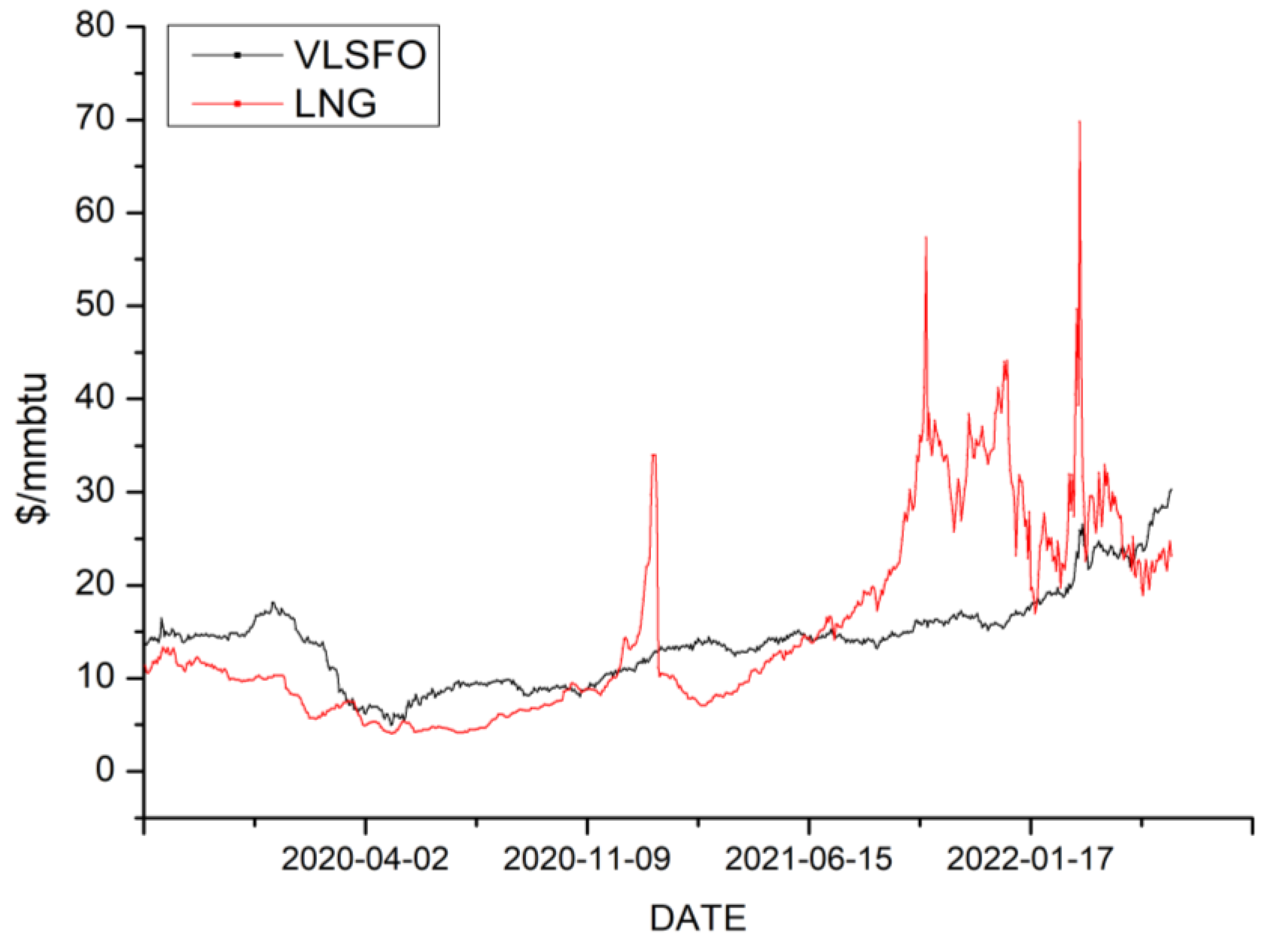
However, shipping companies should pay more attention to satisfying the environmental regulations because these new fuels have high volatilities. The price volatility of VLSFO has been quite high since the regulation of sulfur content limitation. However, as shown in Figure 2, the volatility of LNG bunker prices is higher than that of VLSFO.
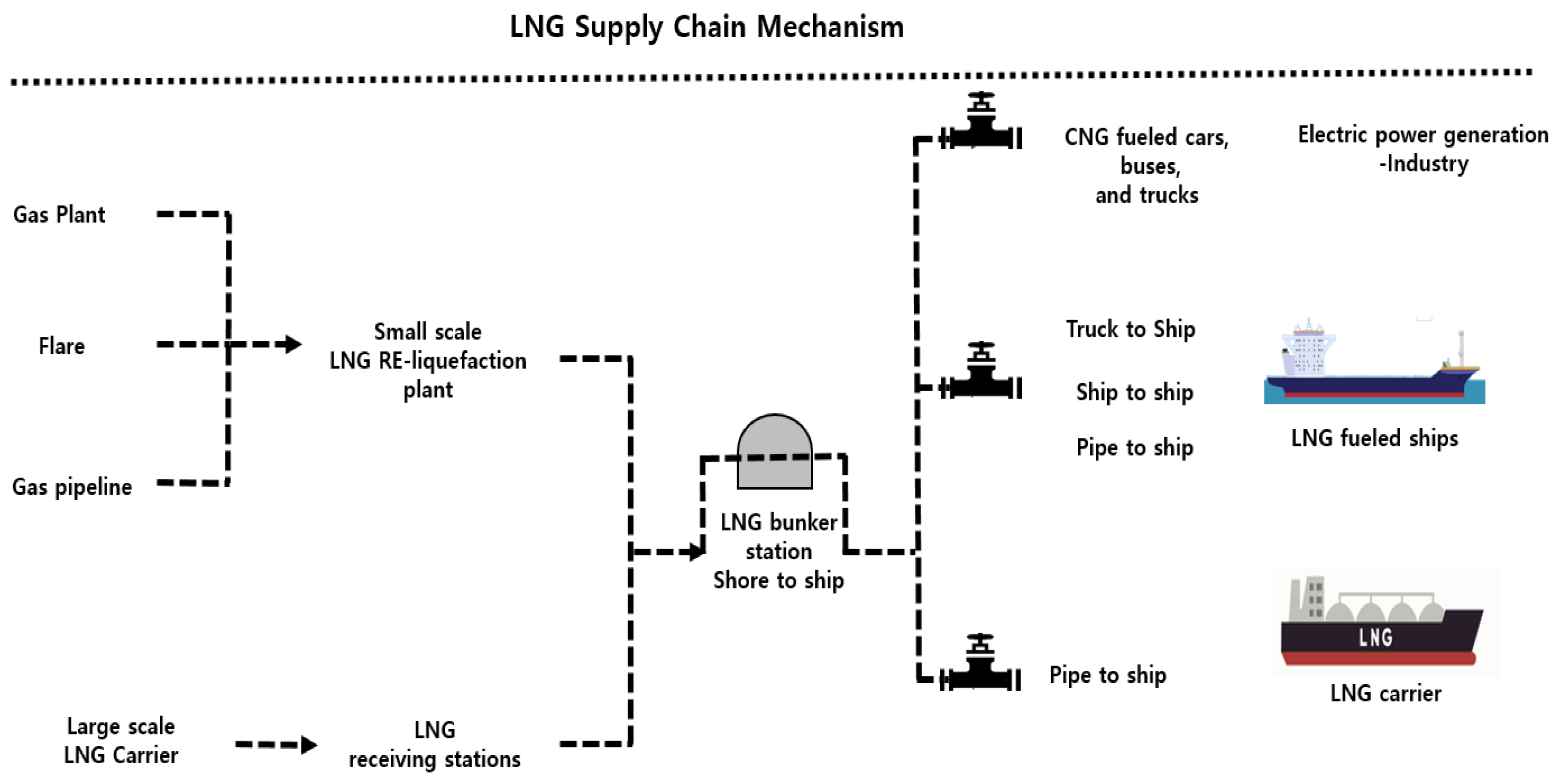
As shown in Figure 3, this is because of the differences in the complexity of the LNG supply chain, transportation and storage processes, political and economic instability, and various port and terminal-related infrastructures. Long-term LNG contract prices in Asia-Pacific are generally determined by oil prices. The LNG market value may not be reflected if the destination of the LNG purchase is restricted or the purchase contract includes a take-or-pay clause. Furthermore, it is difficult for the buyer to flexibly manage procurement, resulting in the decoupling of oil and natural gas prices. Russia’s full-scale invasion of Ukraine has pushed LNG and oil prices to historic highs, as the conflict has resulted in high market volatility and a coordinated global economy. J.P. Morgan’s Global Research Institute has examined the expectations for LNG and oil prices as the possibility of an ongoing conflict poses potential risks to supply chain management [7]. Therefore, shipping companies need to prepare countermeasures based on scientific forecasting techniques, as the LNG bunker price is expected to be more volatile than the marine bunker price in the future.

1.2. Purpose

As discussed earlier, shipping companies have implemented countermeasures such as changing the navigation method to slow steaming, LNG bunker adjustment, using derivative products, and forging long-term agreements for bunker fuel supply to cope with the volatility in the LNG bunker prices. An analysis showed that changing the navigation method to increase fleet sizes while reducing vessel speeds can potentially minimize costs [8]. Furthermore, it has been established that the use of derivative products can have a hedging effect on the volatility of LNG bunker prices [9]. In the end, these competitive advantage countermeasures can be viewed as a way to deal with medium- and long-term volatility. Therefore, a cost management strategy based on short-term LNG fuel price forecasting is required. Because tramp vessels, unlike regular liner vessels, have such options for procuring LNG bunker fuel, it is possible to control costs by determining the time and place of LNG bunker fuel procurement through short-term forecasts of less than a month. Therefore, in this study, we aimed to forecast short-term LNG bunker prices using a recurrent neural network (RNN) model suitable for learning from highly volatile data such as time-series data. We also employed horizontal comparative analysis to investigate forecast-related characteristics through comparative verifications of the RNN models. Our forecast method can potentially assist major global shipping companies in making better business decisions.

1.3. Literature Review

As vessels become larger and faster, comprehensive cost management must be implemented systematically for voyage expenses such as cargo and port costs, in addition to the bunker, crew, ship maintenance, and insurance costs. The LNG bunker cost, in particular, is highly volatile. Hence, LNG bunker prices must be precisely estimated throughout the lifetime of a vessel. A charterer or shipowner can reduce the costs by systematically establishing an LNG bunker procurement plan for each voyage if medium- and long-term forecasting of the prices is possible. Nonetheless, there is relatively little reported research on forecasting LNG bunker prices despite the abundance of studies on forecasting general bunker fuel prices. However, major global shipping companies as well as universities and research institutes are paying increasing attention to the cost management of LNG bunker fuel owing to the recent expansion of the ship emission control areas centering on Europe and the United States and the IMO’s 2020 environmental regulations [10].
Analysis shows that orders for LNG-fueled ships have increased significantly owing to the enforcement of IMO environmental regulations [11]. Accordingly, as shown in Table 1, deliveries of LNG-fueled ships will increase beyond that of conventional oil-fueled ships after 2024; however, delivery of LNG-fueled ships may decrease as the zero-carbon policy expands in the future. Their expansion over the next 10 years means the growth of the LNG bunkering market, and it can be confirmed that global shipping companies are also required to manage LNG bunker costs.
Stefanakos and Schinas [13] performed a predictive analysis of bunker prices using the weekly HSFO 380CST prices at major bunker supply ports, such as Rotterdam, Fujairah, Singapore, and Houston. The vector autoregressive moving average model was employed, which is typically used for financial time-series forecasting. The prediction performance of the models with previous variables added for the one lag of the four ports and the one to four lags of one port for the upcoming third quarter was excellent. Furthermore, the prediction performance for a medium-term analysis over 52 weeks was within 20%. In their other work [14], Stefanikos and Schinas used the fuzzy time-series model to analyze bunker fuel at the same ports after including HSFO 180CST, MDO, and MGO bunker fuel types. The results revealed that the forecast for MDO in Rotterdam performed the worst. Choi used system dynamics [15] to analyze the HSFO 380CST prices using annual data from the Singapore port. Crude oil production and consumption, West Texas Intermediate (WTI), world GDP, exchange rates, cargo demand, supply of vessels, demand/supply ratio, and freight rates were the variables affecting bunker prices. According to the analysis results, the average bunker price between 2017 and 2029 will be 26% higher than that between 1990 and 2015. Kim [16] performed a forecasting analysis of bunker prices using the weekly HSFO 380CST in Singapore. Three recurrent neural network model such as RNN, LSTM, and GRU was employed, which is normally used for time-series data. The prediction performance of RNN was better than others. However it has been different length of sequence for forecasting among models.
Several studies have been conducted based on crude oil prices that have a pattern similar to that of marine fuel oil. An analysis of the performance of an empirical mode decomposition (EMD)-based neural network model and an ARIMA model to predict the daily price of WTI and Brent crude oils revealed excellent results for the neural network model to which EMD was applied [17]. Similarly, for predicting the monthly price of WTI and Brent crude oils, the prediction performance was compared using the support vector machine (SVM), random walk model, ARIMA, fractional integrated ARIMA, Markov-switching ARFIMA, and feed-forward neural network. The Diebold–Mariano test revealed a greater predictive power for SVM in Brent crude oil compared with the other models at a significance level of 5% [18]. In addition, the monthly price of WTI crude oil futures was predicted using the multi-layer back propagation neural network and Harr A trous wavelet decomposition [19]. Furthermore, Salvi et al. [20] used LSTM to predict the daily price of Brent oil, Güleryüz and Özden [21] predicted the weekly prices, and Wu et al. [22] analyzed the WTI daily prices using LSTM with ensemble empirical mode decomposition.
As described above, most of the preceding studies are predictions of crude oil or ship’s bunker oil. Most of the data in the studies used weekly prices. The reason is that the weekly price prediction has the greatest impact on the bunker cost management of the shipping company. In particular, these characteristics are more prominent in the tramp market that does not generally take long-term contracts. Although the methods used for prediction in previous studies are very diverse, there are few studies comparing predictions between recurrent neural networks specialized in time series. Therefore, this study intends to proceed with the study by referring to the contents of these previous studies. Therefore, this study can make a gap from previous studies through the following three characteristics. First, it will be a trial study that conducted the prediction of LNG bunker price with high volatility compared with crude oil or bunker. In addition, the prediction will contribute to the decision-making of shipping companies using the weekly price referenced in previous studies. Second, we will predict three recurrent neural networks specialized in time-series data and compare their performance. Recurrent neural network models are commonly used for time-series data such as price prediction because the previous data are circulated. Therefore, it is possible to verify the effectiveness of the prediction through this models. Third, the recurrent neural network has been called the black box model because it lacks a relatively statistical causal relationship. Therefore, the performance comparison of the predicted values will be statistically supplemented through the Diebold–Mariano test.

2. Materials and Methods

2.1. Data

This study used the weekly prices of LNG bunkers from Singapore, which is the largest LNG bunker hub in Asia. The analysis used 144 weekly time-series data between September 2019 and May 2022. The data were divided into a training and test set in an 8:2 ratio. The data from September 2019 to July 2021 served as the training set, and the data from July 2021 to November 2021 served as the validation set. It is conventional to split the training and test set in a ratio between 7:3 and 8:2 to train neural network models. Consequently, this split was followed in this study. Furthermore, the Collaboratory tool from Google was used to forecast the LNG bunker prices using RNNs and artificial neural networks. The program was implemented using Python and run on GPUs in Google cloud computing environment GPUs. Table 2 lists the descriptive statistics of the data. Time-series data are nonstationary in general. As a result, the data were validated using the augmented Dickey–Fuller (ADF) test. The null hypothesis in this test is that data have a unit root. This means that data are nonstationary. Furthermore, this test does not reject the null hypothesis. As a result, LNG Bunker price data are non-stationary as well. However, artificial neural networks that allow non-linearities would be helpful for this data [23].

2.2. Research Modeling

2.2.1. Simple RNN

The simple RNN model used in this study is designed to analyze time-varying data (i.e., time-series data) and is constructed based on the study by Rumelhart et al. [24]. Unlike a traditional artificial neural network, a simple RNN feeds back a portion of the data between the input and output layers to deliver time-series information. In simple RNN, the output of the hidden layer becomes the input of the next hidden layer again. These layers are commonly referred to as cells. Therefore, the hidden layer vector ( h t ) is expressed in Equation (1) and the output vector ( y t ) is expressed in Equation (2). Here, x t is input vector at time t , W is parameter matrices, vector f becomes one of the nonlinear activation functions, and b is a bias.
h t = t a n h ( W h h t 1 + W x x t + b )
y t = f ( W h h t + b )

2.2.2. LSTM

A conventional simple RNN model has a long-term dependency problem, owing to the vanishing gradient during the training process. A simple RNN model using memory cells was developed to address this issue. The LSTM [25] and GRU models [26] are examples of such a model. The LSTM model employs a memory cell structure that includes a forget gate, an input gate, and an output gate that employ sigmoid and hyperbolic tangent functions to delete unnecessary information while storing essential long-term memory information, allowing LSTMs to use long-term memory information. First, the forget gate is used to determine which cell to discard. As in Equation (3), the forget gate ( f t ) can be acquired, which is derived from the combination of input ( x t ) and old hidden state ( h t 1 ) through a sigmoid function. The input gate is represented by Equations (4) and (5). The input gate determines the new information to be input. This gate is divided into two sections. There is the input gate ( i t ), like f t , and a new long-term candidate ( C ~ t ) through the hyperbolic tangent function. Vectors from the input and the forget gates are entered as new long-term values ( C t ), as exhibited in Equation (6). This is the sum of the product of f t and C t 1 and the product of i t and C ~ t . Finally, the output ( O t ) is calculated similarly to the i t or f t using h t 1 and x t , as shown in Equation (7). The new short-term state value ( h t ) is calculated by multiplying O t and C t derived through the hyperbolic tangent function, as shown in Equation (8). Learning is accomplished in this manner by transmitting the short-term state values h t and C t .
f t = σ ( W x f x t + W h f h t 1 + b f )
i t = σ ( W x i x t + W h i h t 1 + b i )
C ~ t = t a n h ( W x i x t + W x c h t 1 + b c )
C t = f t C t 1 + i t C ~ t
O t = σ ( W x o x t + W h o h t 1 + b o )
h t = O t t a n h ( C t )

2.2.3. GRU

The GRU model consists of a reset gate and an update gate, similar to the LSTM forget gate and input gate combination. A reset gate ( r t ) exists in the GRU model, as shown in Equation (9). The reset gate multiplies the old hidden state ( h t 1 ) and input ( x t ) by weights and outputs 0 or 1 after passing the sigmoid activation function. As shown in Equation (10), the update gate ( Z t ) is similar to the LSTM’s forget gate and input gate combined. Like a reset gate, an update gate ( Z t ) is output based on the weights of h t 1 and x t . Z t determines how much hidden state information from the previous time is used and the present input value is combined with 1 Z t to determine how much present information is reflected. The new candidate hidden state ( h ~ t ), which is between −1 and 1 owing to the hyperbolic tangent function, is composed of the sum of x t and the elementwise multiplication of r t and h t 1 , as expressed in Equation (11). Finally, the amount of information on the old hidden state ( h t 1 ) is calculated using Z t , and the amount of information on the new candidate hidden state ( h ~ t ) is calculated using 1 Z t . As a result, the new hidden state ( h t ) is calculated from the sum of these two parts, as shown in Equation (12).
r t = σ ( W x r x t + W h r h t 1 + b r )
Z t = σ ( W x z x t + W h z h t 1 + b z )
h ~ t = t a n h ( W x h ~ x t + W h h ~ ( r t h t 1 ) + b h ~ )
h t = Z t h t 1 + ( 1 Z t ) h ~ t

2.2.4. Hyper Parameter Modelling

In this study, the three RNN models described above were used for forecasting. A supervised learning problem was constructed using time-series data for forecasting by classifying the time step (t) data to be predicted and the past data at (t − α). Additionally, the previous studies [16,27,28,29] that used neural network model to forecast were consulted to determine the extent of the lag to be used from the past data. As short-term forecasts are based on weekly data, the sequence length of the neural network model was set into 3 based on these studies. Other parameters were set as follows, referring to previous studies [16,20,21,27,28,29] based on recurrent neural networks.
When predicting LNG bunker prices, large-scale numbers must be calculated repeatedly to obtain the price per ton. As a result, the input data were converted into a value between 0 and 1 using a min–max scaler to improve prediction performance. The activation function in the model is a Relu function, which outputs 0 for a negative input and the input itself for positive input. As a result, it solves the problem associated with the use of a sigmoid function. The Adam optimizer, as in previous studies, was used to optimize the model based on the loss function. The Adam algorithm combines the advantages of the momentum and RMSProp algorithms, both of which are adaptive gradient methods. The number of hidden layers was set to one based on previous studies [16,30,31], which concluded that sufficient forecasting capability could be achieved using just one hidden layer. The number of neurons in the hidden layer was fixed at 30 to keep the model concise. The batch size was set to 30 in all models. The learning rate was set to 0.001, which is the default value in the Adam algorithm. For an epoch, determining a suitable number is difficult. Hence, the validation and training sets were compared. The point at which the value of loss function starts to increase for the validation set and the model begins to overfit the training data was used as a reference for early stopping and determining the number of epochs to avoid overfitting. Furthermore, to prevent the validation set’s loss function from abruptly terminating as a result of a change, the training was set to stop only if the loss function had not improved for at least five iterations. The dropout values used were 0.

2.3. Performance Indicators

To compare the prediction performance of the models, mean absolute error (MAE) [32], mean squared error (MSE) [33], root mean squared error (RMSE) [34], and mean absolute percentage error (MAPE) [35] were used as verification indicators. MAE, MSE, RMSE, and MAPE are commonly used indicators to evaluate prediction performances. These indicators are defined as follows:
M A E = 1 n i = 1 n | y i y ^ i | ,
M S E = 1 n i = 1 n ( y i y ^ i ) 2 ,
R M S E = 1 n i = 1 n ( y i y ^ i ) 2 ,
M A P E = 100 n i = 1 n | y i y ^ i y i | ,
where y i and y ^ i are the observed and predicted data, respectively. n is the size of the observed data.
Furthermore, the Diebold–Mariano test [16,17,36] was used to analyze the differences in statistical prediction performances between the models.

3. Results

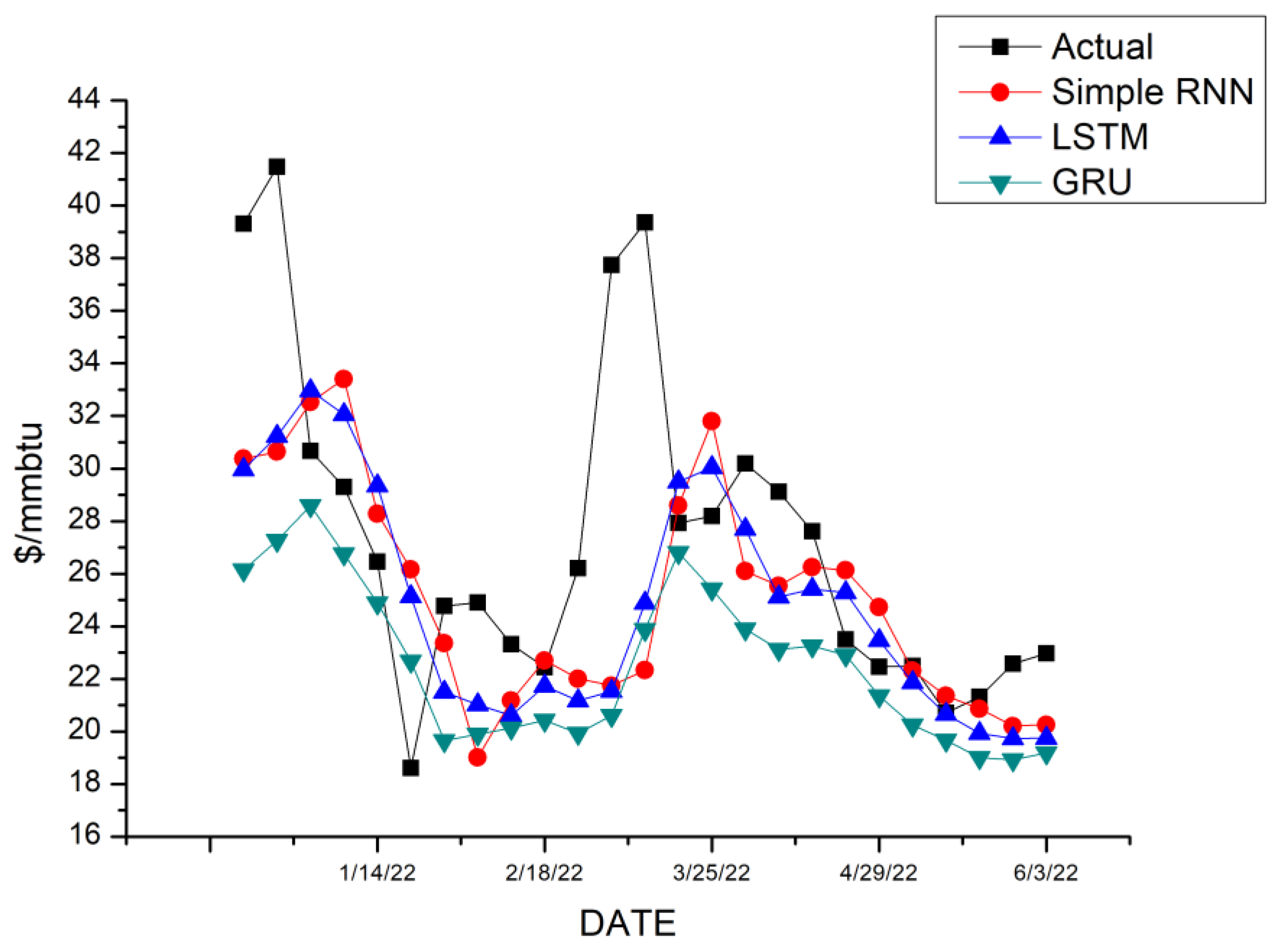
The forecasting was based on the selected hyperparameters. Table 3 shows the verification indicators from the analysis. The results indicate that the LSTM had excellent prediction performance for all the verification indicators (MAE, MSE, MAPE, and RMSE) followed by the simple RNN and GRU. Compared with the simple RNN, the GRU model had relatively low predictive performance in all indicators. The GRU model was relatively overfitted compared with the other models. This is presumed to be because of the relatively small variability of the training set compared with the test set in the data used for analysis. As shown in Figure 4, which expresses the predicted values of each model, GRU had less variability compared with the other models. Accordingly, it showed lower predictive performance for rapidly changing LNG bunker prices. Considering the sudden change in the LNG price at any time, it is estimated that the performance of this prediction characteristic may be relatively inferior to other models in the LNG bunker price prediction.
The Diebold–Mariano test was used to validate the statistical significance of the model performances by varying the loss functions and using the LSTM model as the best model and the simple RNN model as the reference model. The analysis results are listed in Table 4. The LSTM model showed an excellent prediction performance at the 1% significance level compared with GRU based on all loss functions. Unlike previous studies [16], RNN did not show the best performance, but did not have statistical significance with the LSTM model with the best performance. It was found that the simple RNN model showed higher predictive performance than GRU at the 5% significance level based on the loss function excluding the squared error.
In conclusion, the LSTM model performed the best in terms of prediction. In studies on forecasting the prices of crude oil, the LSTM or GRU models generally show excellent prediction performances [21,22,37] because they use long-term memory, which can solve the vanishing gradient problem and use long-term information, making them advantageous for analyzing time-series data, which is affected by past information. In the case of simple RNN, it has relatively high volatility and high sensitivity in a specific range, but owing to excessive sensitivity, it was limited in following the rapidly changing LNG bunker price. In the case of LSTM, however, the sensitivity is somewhat low in a specific range because it reflects a large part of the volatility of the existing LNG bunker price, but it shows high predictive performance when rapidly changing and regressing after a specific range. In the case of GRU, low variability caused by overfitting resulted in poor predictive performance for outliers.

4. Discussion

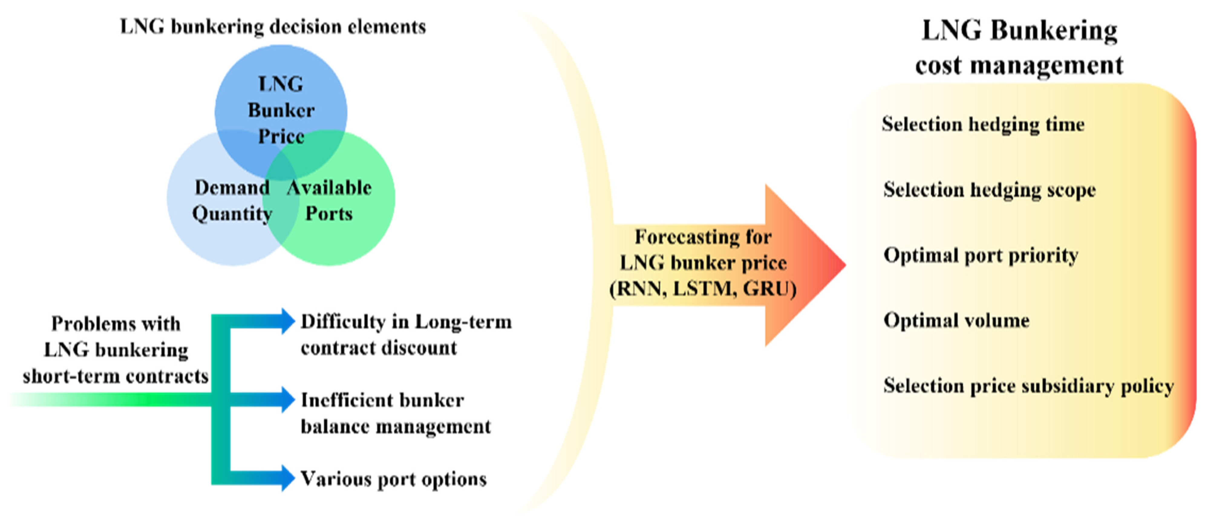
Owing to the intensified sulfur oxide environmental regulations of the IMO, shipping companies have options such as low-sulfur oil, LNG as marine fuel, and scrubber installation. Among these methods, the use of LNG bunker is feasible in the medium- to long-term and, in particular, it has been adopted as the method for the majority of new shipbuilding orders. According to Table 1, orders for LNG-fueled ships are expected to increase over 1~20 years. In addition to these changes, a change in the management method in terms of the cost reduction of shipping companies that have suffered a long-term shipping stagnation following the financial crisis can lead to efficient cost management of LNG bunkers. The main factor in selecting an LNG bunkering port is the suitability for the LNG bunkers price, required quantity, supply and demand, and port regulations, as shown in Figure 5. In general, liners can receive LNG bunkers at a relatively stable price through long-term contracts with specific bunkering companies in specific ports by taking advantage of economies of scale because they have various sailing routes and large fleets. It is easy to calculate the amount required for LNG bunkering in the case of ships sailing on regular routes. However, tramp shipping cannot obtain a discount owing to a long-term contract, and there is a difficulty in determining the supply and demand through various ports in a short-term contract according to a new sailing plan. Therefore, a short-term forecast of the price of LNG bunkers under these circumstances can be helpful. Through short-term forecasting, shipping companies can also consider supply and demand, selection of supply and demand ports, and the size and timing of hedge contracts.
However, natural gas, which is a raw material for LNG bunkering linked to the price of LNG bunkering, has very high volatility compared with crude oil owing to the influence of seasonal factors and political and industrial factors. Therefore, the LNG bunker price, which has high volatility and non-linear characteristics, was analyzed with a recurrent neural network model with high predictive ability. As a result of analyzing three recurrent neural network models, simple RNN, LSTM, and GRU, the predictive performance of LSTM using long-term memory was analyzed to be relatively high. Shipping companies create additional economic benefits by considering various factors such as ship operation, port characteristics, cargo management, weather conditions, and prices of alternative fuels, as well as predictability based on a predictive model that considers only the characteristics of LNG bunkering prices. This study has limitations in determining the economic advantages and differences by applying the simple RNN, LSTM, and GRU models, respectively. Through this study, it is expected that the volatility of LSTM will be significant in the prediction of the LNG bunker price, which shows high volatility without a one-way trend. Finally, this study is expected to contribute to establishing a systematic strategy for supervisors in global shipping companies, port authorities, and LNG bunkering companies.

5. Conclusions

Generally, marine fuel oil is an important cost item that makes up for 47% of an average ship’s operating cost [2]. The LNG bunkering price is highly volatile and, because of the high dynamics, it is necessary to accurately estimate the price during the operation period of the vessel.
To academically solve these practical problems, this study investigated methods for obtaining short-term LNG bunker price forecasts, which can be used by shipping companies as an effective cost-control measure for the cost associated with LNG bunkers. LNG bunker fuel procurement decisions based on short-term responses play a critical role in managing the expenses of shipping companies. These short-term responses necessitated the forecasting LNG bunker prices. Predictive analysis was performed using simple RNN, LSTM, and GRU models, which are effective in forecasting time-series data.
First, LSTM showed the best prediction performance among the three models based on indicators such as MAE, MSE, MAPE, and RMSE. LSTM was followed by simple RNN and GRU. GRU was determined to be relatively overfitted compared with the other models. As the LNG bunkering price data used in the analysis showed high volatility in recent years, it is assumed that overfitting deteriorated the forecasting performance. However, LSTM and simple RNN showed relatively good predictive performance for the test set despite such variability.
Second, the Diebold–Mariano test was performed to statistically estimate the prediction accuracy of the prediction value. As a result, it was analyzed that LSTM showed excellent predictive performance at the 1% significance level compared with GRU. However, LSTM was not found to be statistically superior to simple RNN. In comparing simple RNN to GRU, simple RNN was analyzed to be statistically superior at the 5% significance level based on absolute error and square proportional error. Therefore, it was determined that GRU has a significantly lower predictive performance compared with the other models.
To the best of our knowledge, this study was the first to analyze the LNG bunker prices using simple RNN models. Hence, this study merits academic significance. Furthermore, it was possible to effectively manage ship operating costs in practice for their own fleet by improving the accuracy of short-term bunker price forecasts. This study was limited by the vague standard for adjusting the model hyperparameters. In future research, we aim to improve the performance by investigating the selection of hyperparameters. These hyperparameters can then be used to search for a set of parameters that correspond to the set of data needed to make business decisions by categorizing various factors that influence the fluctuation in LNG bunker prices.

Author Contributions

Conceptualization, K.K. and S.L.; Methodology, K.K. and S.L.; Validation, C.-h.L. and S.L.; Investigation, S.L. and D.J.; Resources, K.K. and W.-J.L.; Data Curation, D.J.; Writing Preparation, S.L. and C.-h.L.; Writing—Review and Editing J.J., K.K., H.J., and C.-h.L.; Visualization, J.J., K.K., H.J., and W.-J.L.; Supervision, S.L. and C.-h.L.; Project Administration, S.L. and H.J.; Funding Acquisition, H.J., C.-h.L., D.J., and W.-J.L. All authors have read and agreed to the published version of the manuscript.

Funding

This study was supported by a grant from the National R&D Project, “Development of LNG Bunkering Operation Technologies Based on Operation System and Risk Assessment,” funded by the Ministry of Oceans and Fisheries, South Korea, grant number PMS4310; this research was supported by Korea Institute of Marine Science and Technology Promotion (KIMST) funded by the Ministry of Oceans and Fisheries, grant number 20220603.

Institutional Review Board Statement

Not applicable.

Informed Consent Statement

Not applicable.

Data Availability Statement

Not applicable.

Conflicts of Interest

The authors declare no conflict of interest. The funder had no role in the design of the study; in the collection, analyses, or interpretation of data; in the writing of the manuscript; or in the decision to publish the results.

References

  1. Wang, S.; Meng, Q.; Liu, Z. Bunker consumption optimization methods in shipping: A critical review and extensions. Transp. Res. Part E Logist. Transp. Rev. 2013, 53, 49–62. [Google Scholar] [CrossRef] [Green Version]
  2. Stopford, M. Maritime Economics 3e; Routledge: London, UK, 2009. [Google Scholar]
  3. Notteboom, T.E.; Vernimmen, B. The effect of high fuel costs on liner service configuration in container shipping. J. Transp. Geogr. 2009, 17, 325–337. [Google Scholar] [CrossRef]
  4. Alizadeh, A.H.; Nomikos, N.K. Shipping Derivatives and Risk Management; Palgrave Macmillan: London, UK, 2009; ISBN 978-0-230-21591-7. [Google Scholar]
  5. Clarkson Research Shipping Intelligence Network. Available online: https://sin.clarksons.net/ (accessed on 19 March 2022).
  6. Platts bunkerwire. Available online: https://www.spglobal.com/commodityinsights/en/products-services/shipping/bunkerwire (accessed on 28 September 2022).
  7. Available online: https://www.jpmorgan.com/insights/research/oil-gas-energy-prices (accessed on 28 September 2022).
  8. Ronen, D. The effect of oil price on containership speed and fleet size. J. Oper. Res. Soc. 2011, 62, 211–216. [Google Scholar] [CrossRef]
  9. Alizadeh, A.H.; Kavussanos, M.G.; Menachof, D.A. Hedging against bunker price fluctuations using petroleum futures contracts: Constant versus time-varying hedge ratios. Appl. Econ. 2004, 36, 1337–1353. [Google Scholar] [CrossRef]
  10. Qi, J.; Wang, H.; Zheng, J. Promoting liquefied natural gas (LNG) bunkering for maritime transportation: Should ports or ships be subsidized? Sustainability 2022, 14, 6647. [Google Scholar] [CrossRef]
  11. Livaniou, S.; Chatzistelios, G.; Lyridis, D.V.; Bellos, E. LNG vs. MDO in marine fuel emissions tracking. Sustainability 2022, 14, 3860. [Google Scholar] [CrossRef]
  12. Lloyd’s Register Advisory Service Korea LNG Bunkering Review (Busan, Incheon, and Ulsan Ports). 2022.
  13. Stefanakos, C.N.; Schinas, O. Forecasting bunker prices; A nonstationary, multivariate methodology. Transp. Res. Part C Emerg. Technol. 2014, 38, 177–194. [Google Scholar] [CrossRef]
  14. Stefanakos, C.; Schinas, O. Fuzzy time series forecasting of bunker prices: Nonstationary considerations. WMU J. Marit. Aff. 2015, 14, 177–199. [Google Scholar] [CrossRef]
  15. Choi, J. Forecasting Bunker Price Using System Dynamics. J. Korea Port Econ. Assoc. 2017, 33, 75–87. [Google Scholar] [CrossRef]
  16. Kim, K. A Study on the Forecasting of Bunker Price Using Recurrent Neural Network. J. Korea Soc. Comput. Inf. 2021, 26, 179–184. [Google Scholar] [CrossRef]
  17. Yu, L.; Wang, S.; Lai, K.K. Forecasting crude oil price with an EMD-based neural network ensemble learning paradigm. Energy Econ. 2008, 30, 2623–2635. [Google Scholar] [CrossRef]
  18. Yu, L.; Zhang, X.; Wang, S. Assessing potentiality of support vector machine method in crude oil price forecasting. Eurasia J. Math. Sci. Technol. Educ. 2017, 13, 7893–7904. [Google Scholar] [CrossRef]
  19. Jammazi, R.; Aloui, C. Crude oil price forecasting: Experimental evidence from wavelet decomposition and neural network modeling. Energy Econ. 2012, 34, 828–841. [Google Scholar] [CrossRef]
  20. Salvi, H. Long short-term model for brent oil price forecasting. Int. J. Res. Appl. Sci. Eng. Technol. 2019, 7, 315–319. [Google Scholar] [CrossRef]
  21. Güleryüz, D.; Özden, E. The prediction of Brent crude oil trend using LSTM and Facebook prophet. Avrupa Bilim Ve Teknol. Derg. 2020, 1–9. [Google Scholar] [CrossRef]
  22. Wu, Y.; Wu, Q.; Zhu, J. Improved EEMD-based crude oil price forecasting using LSTM networks. Physica A 2019, 516, 114–124. [Google Scholar] [CrossRef]
  23. Manowska, A.; Bluszcz, A. Forecasting Crude Oil Consumption in Poland Based on LSTM Recurrent Neural Network. Energies 2022, 15, 4885. [Google Scholar] [CrossRef]
  24. Rumelhart, D.E.; Hinton, G.E.; Williams, R.J. Learning representations by back-propagating errors. Nature 1986, 323, 533–536. [Google Scholar] [CrossRef]
  25. Hochreiter, S.; Schmidhuber, J. Long short-term memory. Neural Comput. 1997, 9, 1735–1780. [Google Scholar] [CrossRef]
  26. Cho, K.; van Merrienboer, B.; Gulcehre, C.; Bahdanau, D.; Bougares, F.; Schwenk, H.; Bengio, Y. Learning Phrase Representations using RNN Encoder-Decoder for Statistical Machine Translation. 2014. Available online: https://arxiv.org/abs/1406.1078 (accessed on 28 September 2022).
  27. Kim, D.; Kim, H.; Sim, S.; Choi, Y.; Bae, H.; Yun, H. Prediction of dry bulk freight index using deep learning. J. Korean Inst. Ind. Eng. 2019, 45, 111–116. [Google Scholar] [CrossRef]
  28. Han, M.; Yu, S. Prediction of Baltic Dry Index by Applications of Long Short-Term Memory. J. Korean Soc. Qual. Manag. 2019, 47, 497–508. [Google Scholar]
  29. Lim, S.; Yun, H. Forecasting bulk market indices with recurrent neural network models. J. Marit. Bus. 2018, 40, 159–180. [Google Scholar]
  30. Cybenko, G. Approximation by superpositions of a sigmoidal function. Math. Control Signals Syst. 1989, 2, 303–314. [Google Scholar] [CrossRef]
  31. Zhang, G.; Patuwo, B.E.; Hu, M.Y. Forecasting with artificial neural networks: The state of the art. Int. J. Forecast. 1998, 14, 35–62. [Google Scholar] [CrossRef]
  32. Willmott, C.J.; Matsuura, K. Advantages of the mean absolute error (MAE) over the root mean square error (RMSE) in assessing average model performance. Clim. Res. 2005, 30, 79–82. [Google Scholar] [CrossRef]
  33. Wallach, D.; Goffinet, B. Mean squared error of prediction as a criterion for evaluating and comparing system models. Ecol. Model. 1989, 44, 299–306. [Google Scholar] [CrossRef]
  34. Chai, T.; Draxler, R.R. Root mean square error (RMSE) or mean absolute error (MAE)?—Arguments against avoiding RMSE in the literature. Geosci. Model Dev. 2014, 7, 1247–1250. [Google Scholar] [CrossRef] [Green Version]
  35. de Myttenaere, A.; Golden, B.; Le Grand, B.; Rossi, F. Mean absolute percentage error for regression models. Neurocomputing 2016, 192, 38–48. [Google Scholar] [CrossRef] [Green Version]
  36. Diebold, F.X.; Mariano, R.S. Comparing predictive accuracy. J. Bus. Econ. Stat. 2002, 20, 134–144. [Google Scholar] [CrossRef]
  37. Lin, H.; Sun, Q. Crude oil prices forecasting: An approach of using ceemdan-based multi-layer gated recurrent unit networks. Energies 2020, 13, 1543. [Google Scholar] [CrossRef]
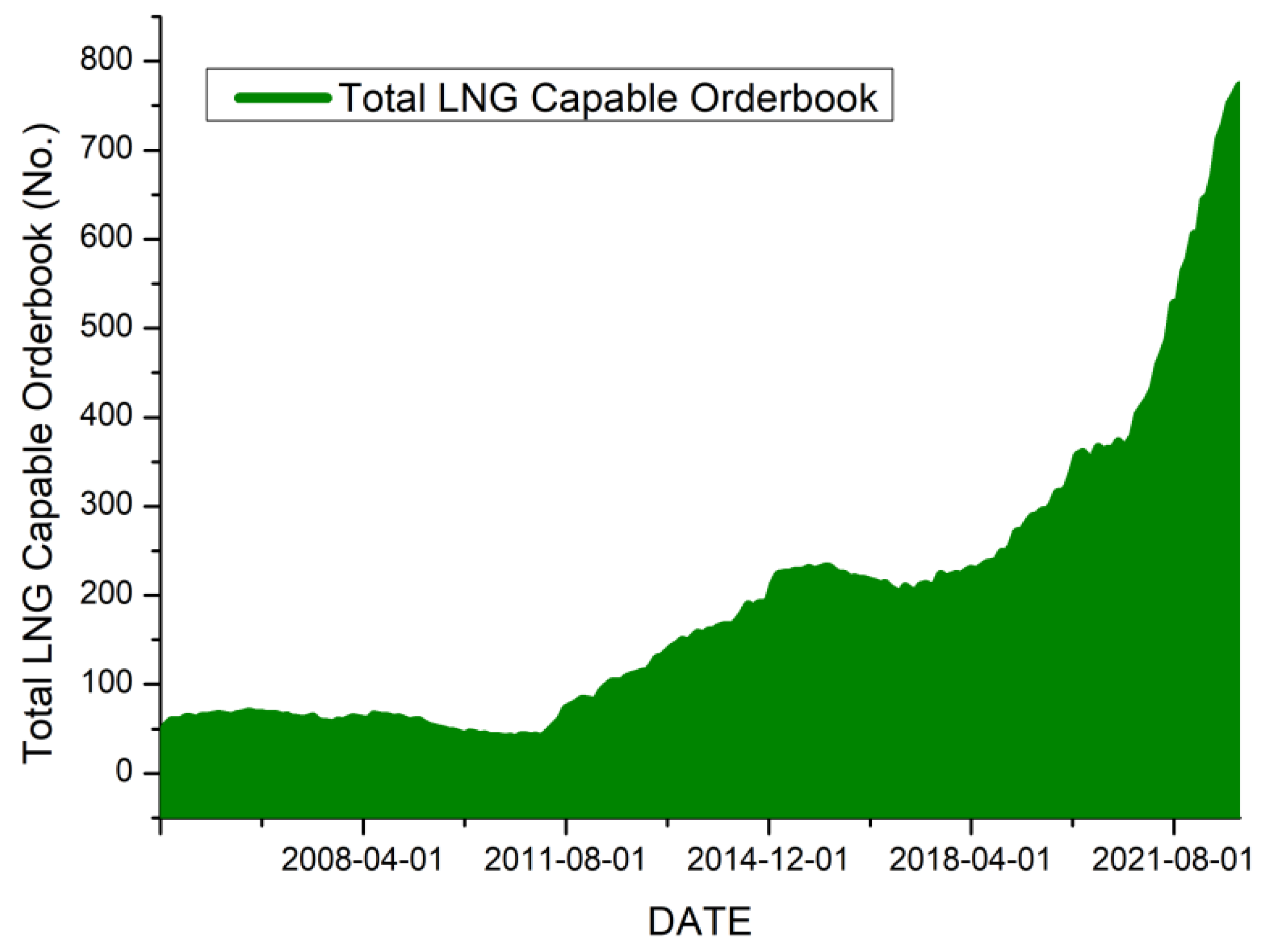
Figure 1. LNG-capable orderbook trend (adapted from Clarkson research [5]). LNG, liquefied natural gas.
Jmse 10 01814 g001
Figure 2. LNG bunker price trend in the port of Singapore (computed by the authors using data from Platts Bunkerwire [6]). LNG, liquefied natural gas; VLSFO, very low sulfur fuel oil.
Jmse 10 01814 g002
Figure 3. LNG supply chain overview. LNG, liquefied natural gas.
Jmse 10 01814 g003
Figure 4. Prediction of LNG bunker price by each method. RNN, recurrent neural network; LSTM, long short-term memory; GRU, gated recurrent unit.
Jmse 10 01814 g004
Figure 5. LNG bunkering cost management using short-term forecasting.
Jmse 10 01814 g005
Table 1. LNG-fueled ship and decarbonisation scenario.
PeriodPrediction
Early 2020sGradual ramp up of deliveries of LNG-fueled ships
2024–2030LNG-fueled ship deliveries begin to surpass those of conventional oil-fueled ships
2030sLNG-fueled ships shares begin to fall as zero-carbon technologies develop
2040sZero-carbon vessels account for the major share of shipyard output
Source: author revised based on LNG Bunkering Review (Busan, Incheon, and Ulsan Ports) [12]. 2022. LNG, liquefied natural gas.
Table 2. Descriptive statistics of liquefied natural gas bunker prices.
StatisticsWeekly LNG Bunker Price
Observations144
Mean15.04
Std. error0.83
Median11.09
Std. dev.10.00
ADF testt-stat.−1.85
Prob0.353
Source: Computed by the authors using data from Platts Bunkerwire [6].
Table 3. Performance of the proposed models.
ModelMAEMSEMAPERMSE
Simple RNNTr1.17611.812.45
Te4.2638.1314.146.18
LSTMTr1.235.7512.192.4
Te4.1433.8113.775.82
GRUTr1.155.2612.12.29
Te5.0947.5216.816.89
Tr and Te mean training set and test set, respectively. RNN, recurrent neural network; LSTM, long short-term memory; GRU, gated recurrent unit; MAE, mean absolute error; MSE, mean squared error; MAPE, mean absolute percentage error; RMSE, root mean squared error.
Table 4. Diebold–Mariano test results.
BenchmarkSquared ErrorAbsolute ErrorSquared Proportional Error
Simple RNNGRUSimple RNNGRUSimple RNNGRU
LSTM−1.254
(0.105)
−2.623
(0.004)
−0.577
(0.282)
−3.159
(0.001)
−1.029
(0.152)
−3.289
(0.001)
Simple RNN −1.576
(0.058)
−2.160
(0.015)
−1.702
(0.044)
( ) is a p-value, RNN, recurrent neural network; LSTM, long short-term memory; GRU, gated recurrent unit.
Publisher’s Note: MDPI stays neutral with regard to jurisdictional claims in published maps and institutional affiliations.