1. Introduction
The health of the ship is a prerequisite for navigation. At present, in the field of ship health monitoring, fault diagnosis is mainly carried out for bearings, diesel engines and other parts of various ship systems [
1,
2]. However, the hydraulic system is the main component of the main equipment, such as steering gear, fin stabilizers, main propulsion device, deck machinery, etc. The health status of the hydraulic system is of great significance for the fault diagnosis of ship equipment. As the working medium of the hydraulic system, the pollutants contained in the hydraulic oil contain important information about the operating state of the equipment [
3,
4]. According to statistics, more than 75% of mechanical failures of hydraulic systems were caused by hydraulic-oil particulate pollutants [
5]. Analyzing the information of particulate pollutants in marine hydraulic oil comprehensively and accurately has a great significance for the fault diagnosis of hydraulic systems [
6].
Oil-particle detection mainly includes magnetic-based oil-particle detection, acoustic-based oil-particle detection, and optical-based oil-particle detection. Magnetic-based oil-particle detection methods mainly include inductive and capacitive particle sensors. An inductive particle sensor can measure the change of coil inductance when particles pass through. In this way, ferromagnetic particles and non-ferromagnetic wear particles in oil are distinguished and detected. It can obtain particle size but cannot detect non-metallic pollutants with high accuracy [
7,
8,
9]. A capacitive particle sensor can detect non-metallic particle pollutants. However, metal particle pollutants cannot be detected separately [
10,
11], and neither method can identify specific characteristics, such as the shape of oil particles. Although acoustic wave-based oil-particle detection can distinguish between metal particles and bubbles, it cannot distinguish between ferromagnetic and non-ferromagnetic metal particles. More than that, it is incredibly vulnerable to interference from external environments such as temperature and noise, and it is also challenging to obtain specific characteristics of oil particles [
12,
13]. Optical-based oil-particle detection is mainly divided into photoelectric and optical imaging sensors. Photoelectric sensors mainly use laser or uniform light to detect large flux particles and small particles through light scattering or shading. The detection accuracy is high, but it is easily affected by bubbles and light refraction [
14,
15,
16]. The above oil-particle detection methods have a fatal disadvantage; that is, the specific characteristics of oil particles cannot be obtained, and only some simple differentiation or counting can be carried out. In the field of obtaining the specific characteristics of oil particles, the methods based on optical imaging sensors are mainly used at present.
The optical imaging sensor extracts the image through the imaging sensor, then processes the image through an algorithm. Liu et al. designed a microfluidic channel conducive to observing the movement characteristics of particles, then used the Gaussian mixture model (GMM) and the blob-tracking algorithm to realize particle tracking [
17]. Wang et al. used an iron spectrometer to obtain the wear-particle image and proposed a new non-reference method for the objective evaluation of wear-particle edge detection to achieve the contour extraction of wear particles [
18]. Jia et al. used an iron spectrometer and optical microscope to obtain the image of wear particles and designed convolutional neural network (DCNN) models to identify seven kinds of wear particles [
19].
It can be seen that in the field of particle detection of optical imaging sensors, the current mainstream method is to process particle images through traditional image processing or depth learning to obtain particle information. In the traditional image processing field of particle detection, an iron spectrometer is often used to obtain images, but only some particle counting or edge detection operations are carried out, and the particle feature information obtained is also relatively limited. Furthermore, the volume of the iron spectrometer is large, so it is difficult to realize real-time detection. Moreover, obtaining representative particles of non-magnetic and non-metallic particles is difficult, and it is easy to calculate errors [
20,
21]. Due to the rapid development of depth learning, many researchers choose to use depth learning methods to achieve particle detection [
22,
23]. However, when the amount of data is relatively small, the use of depth learning methods can easily lead to overfitting [
24,
25]. For example, to identify four types of particles, where each particle has three features, it is necessary to provide particle images with 12 different features, and the amount of particle image data of each type should be large enough. The labor cost of this method is relatively high [
26], and often the trained model is only suitable for a single scene. If the environment changes, the model needs to be retrained.
To solve the above problems, this paper proposed a method based on OpenCV to identify the particle pollutants in hydraulic oil, as an extension of the traditional particle image processing field. Instead of using an iron spectrometer to obtain a particle pollutants image, CCD is used to obtain the image of particle contamination in hydraulic oil. Moreover, it is no longer just to realize the technology of particles and the function of edge detection. Instead, a series of specific characteristics such as specific size, area, perimeter and shape of particles in oil are successfully detected through morphological processing, contour extraction and shape detection. Additionally, the algorithm has strong applicability. It can realize the real-time online monitoring of oil without complex equipment and instruments.
2. Materials and Methods
2.1. Oil Particle Image Detection Platform
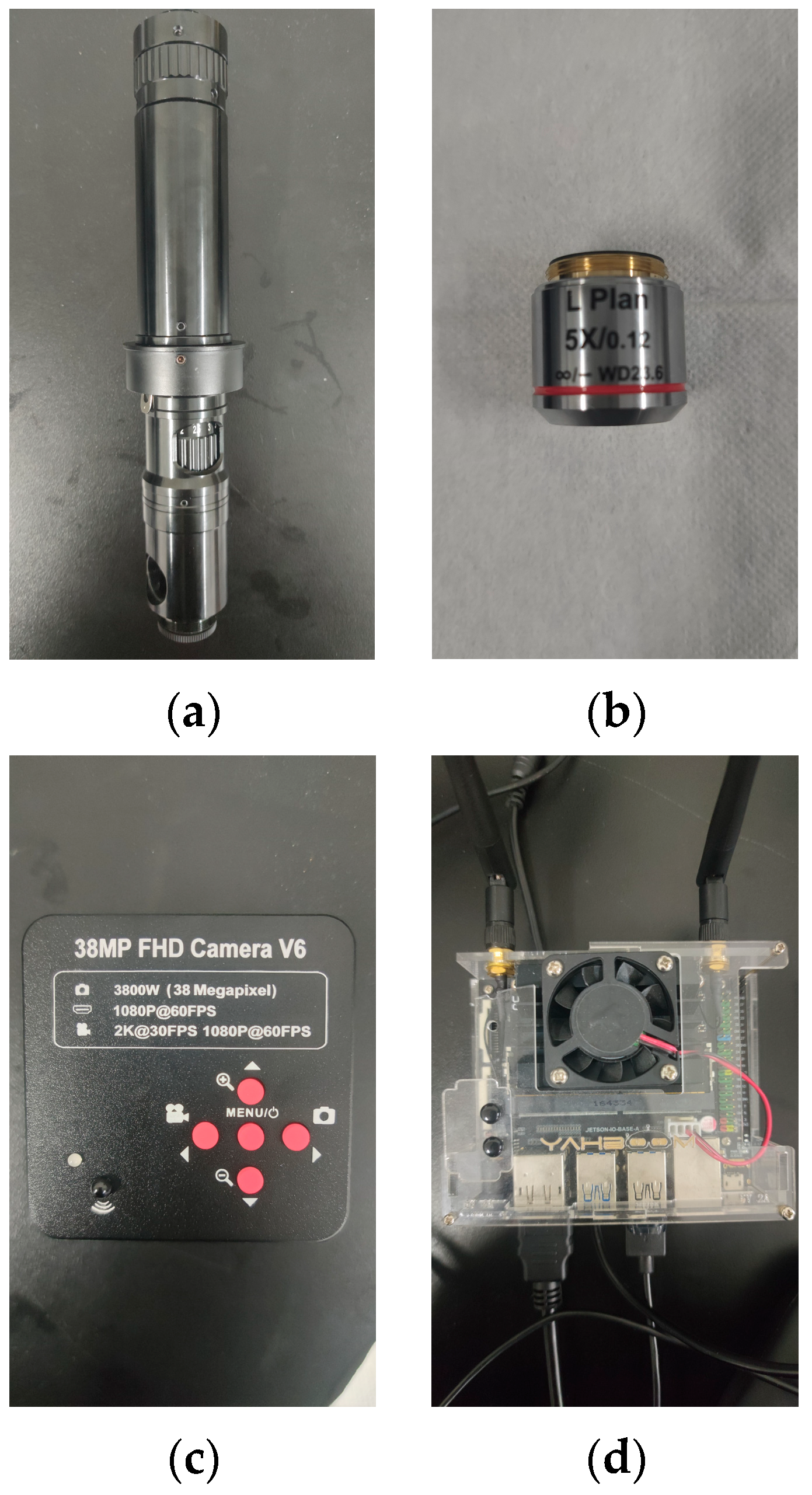
In order to obtain oil particle pictures, an oil-particle-detection platform needs to be built. In order to facilitate its integration into the subsequent miniaturization devices, this paper used a small coaxial optical industrial microscope (
Figure 1a), objective lens (
Figure 1b) and CCD image sensor (
Figure 1c) to replace the large microscope and ferrograph.
The image collected by the CCD image sensor communicates with Nvidia’s Jetson Nano device (
Figure 1d) through a USB interface. The device has a GPU to facilitate subsequent image processing operations. After image processing, the image will be transmitted to the display screen through the antenna on the device.
The whole platform is as shown in
Figure 2.
2.2. Image Morphology Processing
Particle contaminants in oil contain rich information of the state of equipment, but the particle image obtained from oil by the CCD image sensor cannot directly extract its information. It is necessary to apply OpenCV to perform a series of morphological processing steps on the image, to facilitate subsequent operations.
2.2.1. Grayscale and Binarization
A pixel is the smallest unit in an image, and each pixel is mainly represented by three primary colors: R, G, and B (red, green, and blue). In OpenCV, the three components of each pixel have fixed values, so each preprocessed image is represented by a three-dimensional matrix of which the size is three times the total pixels. Before the image’s morphological processing, it is necessary to undertake grayscale and binarization steps on the image to facilitate subsequent operations.
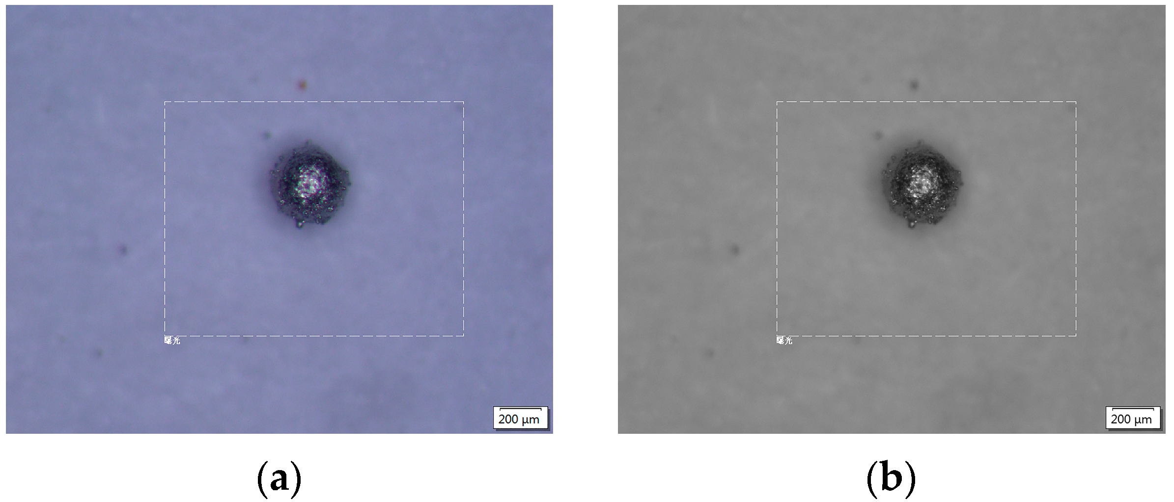
Grayscale transforms the original three-channel image, with R component matrix, G component matrix, and B component matrix, into a single-channel matrix, with R equal to G equal to B component. Compared with the original color image, the grayscale image has the advantages of high processing efficiency and a small footprint. Since the sensitivity of human eyes to color is different, blue is the lowest, red is the medium, and green is the highest, so the weighted-mean method, as shown in Equation (1), is used to grayscale the image.
The original image of oil particles and the grayscale image are shown in
Figure 3.
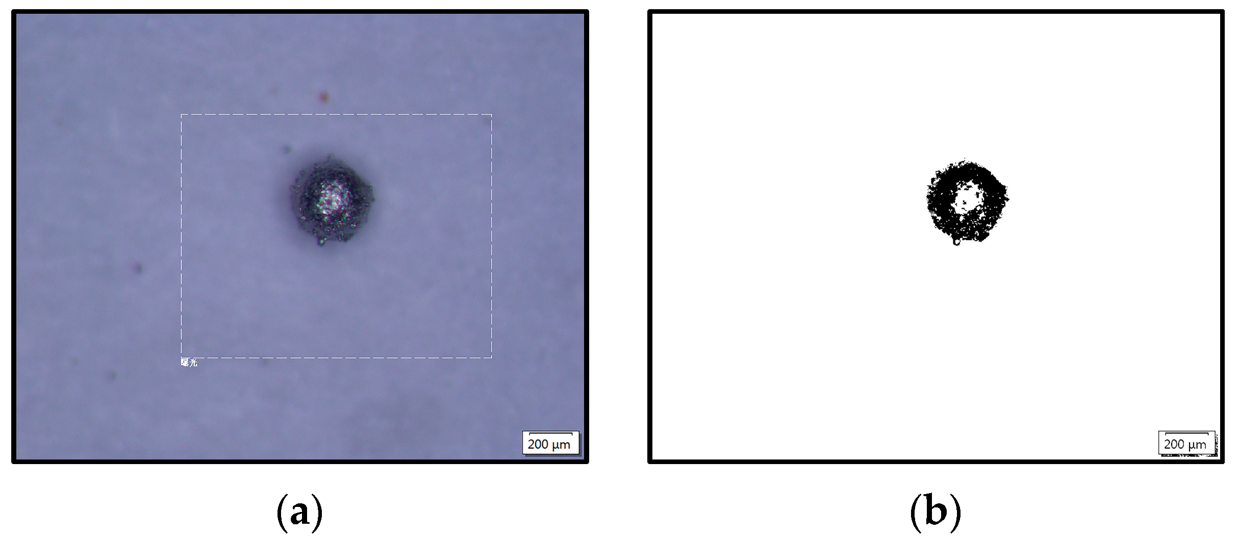
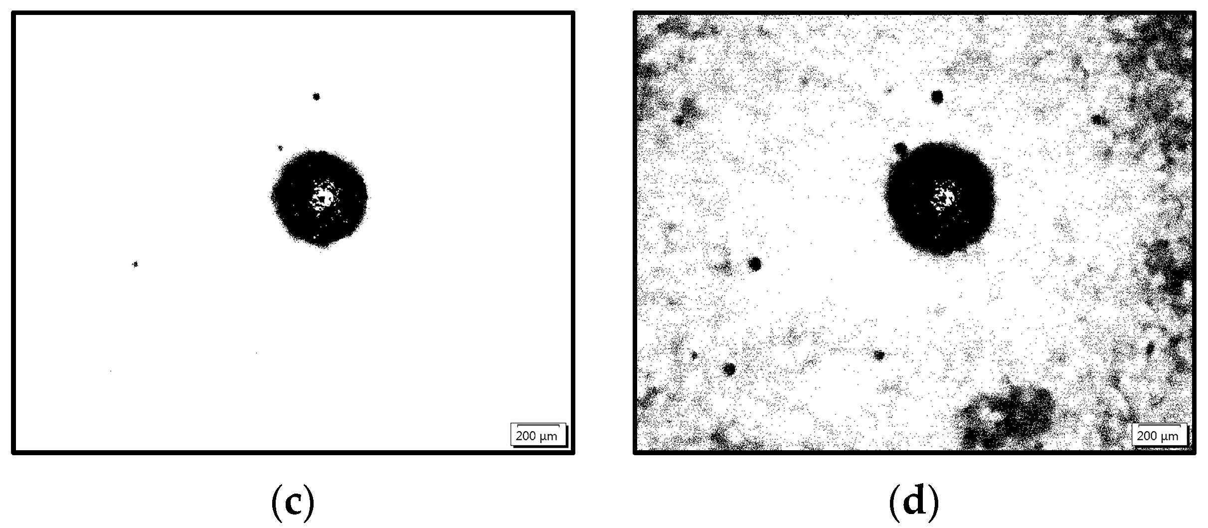
The oil particle image needed to be binarized to simplify the image further. Binarization is to set the gray value to 0 or 255 based on grayscale to convert it to a black and white image for highlighting its contour features. The binarization operation with different thresholds will obtain different results. The binarized images with different thresholds are shown in
Figure 4.
2.2.2. Opening/Closing
According to
Figure 4, after binarization and threshold adjustment, some noise points will still affect subsequent operations.
The opening operation erodes an image and then dilates the eroded image. It can remove isolated minor points and burrs without changing the size and position of the particles, so it achieves the purpose of eliminating noise points. Closing is a process in which first a dilation operation is performed and then an erosion operation is performed, which can help close small holes or flaws on the object and facilitate subsequent contour extraction operations. Similarly, it is also essential to reasonably adjust the number of opening/closing operations. Many tests found that in this application scenario, the best image effect can be obtained after two opening operations and then four closing operations. The images after the operation are shown in
Figure 5.
2.3. Oil Particle Contour Extraction
The most important thing for analyzing the particles in the oil is to extract their characteristics, including the oil particle area, perimeter, shape, and other characteristic parameters, and contour extraction is the premise of obtaining these parameters.
It requires an edge detection algorithm to obtain the contours of oil particles. Common edge detection algorithms include Robert edge detection, Prewitt edge detection, Sobel edge detection, Canny edge detection, and other methods. Among them, the Canny edge detection algorithm is an excellent edge detection algorithm in theory. It has many applications, so in this paper the Canny edge detection algorithm was used to realize the contour extraction function.
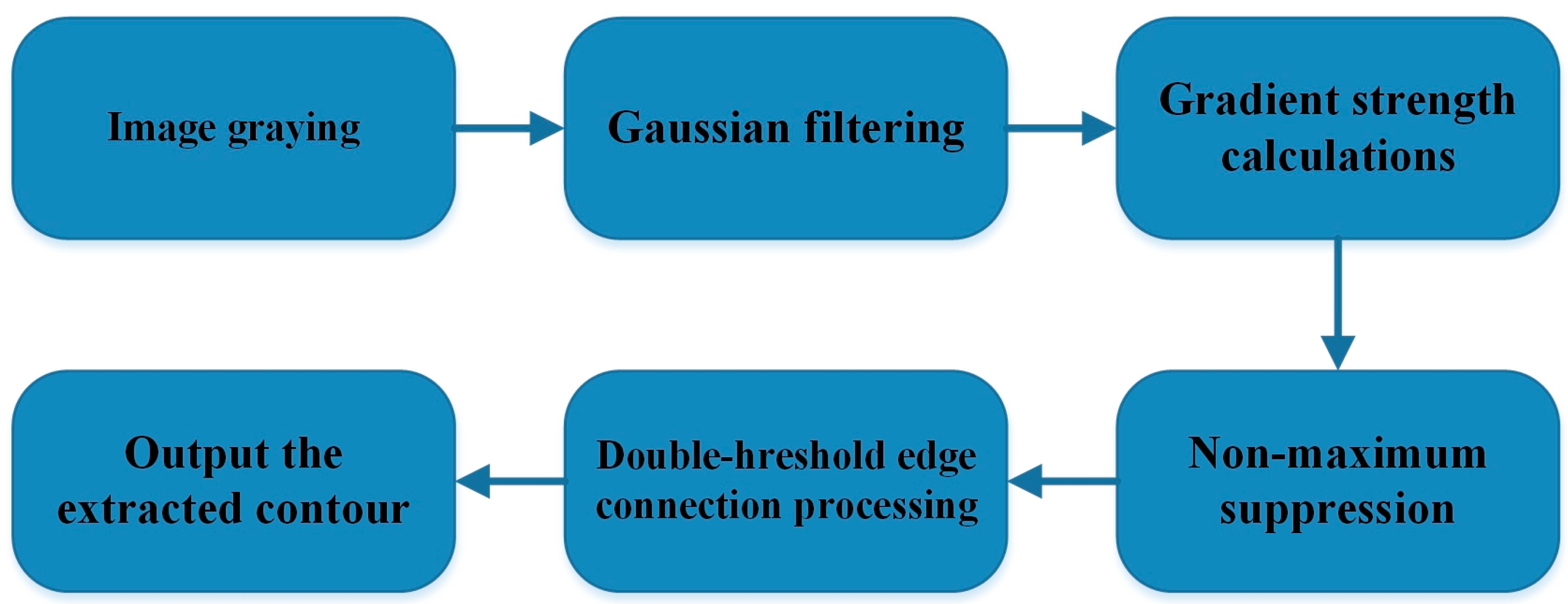
The overall technical roadmap of the Canny edge detection algorithm is shown in
Figure 6. Before contour extraction, the algorithm first performs a series of image morphology processing steps, such as image graying, Gaussian filtering, and denoising, which facilitates subsequent operations. The algorithm then screens the edges of possible oil contamination through gradient strength calculations. After that, the algorithm will use non-maximum suppression and double-threshold edge-connection processing operations to reduce the probability of false detection. Finally, it will output the extracted contour, then calculate the perimeter and area of the contour.
2.3.1. Canny Edge Detection and Contour Extraction
The edge detection algorithm is easily affected by various kinds of noise in the image. Therefore, the Canny edge detection algorithm will start with the Gaussian filtering on the grayscale image, and it will smooth the image and achieve the effect of denoising. The equation of Gaussian filtering is shown in (2).
where f(x,y) is the original image function.
Next, the Canny edge detection algorithm looks for the place with the strongest gradient (the place with the strongest change) in the entire image and marks it as a possible edge pixel. The gradient of each pixel is obtained by using the Sobel operator. The Sobel operator shown in Equation (3) is used to convolve each pixel in the image to obtain the first-order gradient of the image and then set an appropriate threshold to determine whether the point is an edge point.
where S
x and S
y are horizontal direction and vertical direction of the Sobel operator.
The gradient components of x direction and y direction are shown in Equation (4).
The gradient amplitude and direction at point (x, y) are shown in Equations (5) and (6).
The Sobel operator may cause misjudgment of edge points because many noise points also have large gradients. Therefore, the Canny edge detection method will apply non-maximum suppression technology on the pixels after the operation to eliminate the edge misdetection phenomenon.
Non-maximum suppression compares the gradient strength of the pixel with a positive gradient direction pixel and a negative gradient direction pixel. If the gradient strength of this point is the largest, it will be retained. Otherwise, it will be suppressed (set to 0). This method can clarify the original blurred boundary and eliminate some falsely detected edge points.
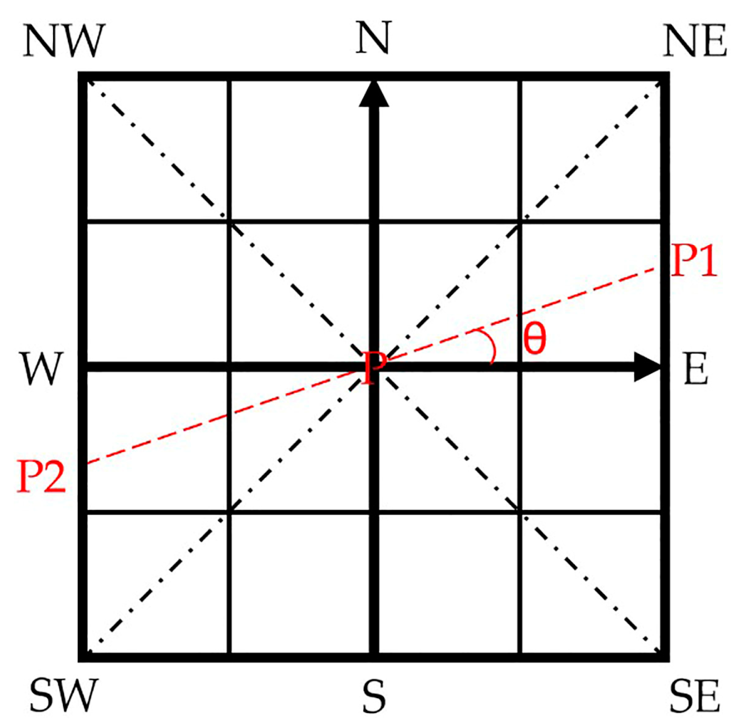
As shown in
Figure 7, to improve the calculation accuracy, linear interpolation is used between two adjacent pixels to obtain the pixel gradient that needs to be compared.
In
Figure 7, E, NE, N, NW, W, SW, S, and SE are the pixel points corresponding to different directions of the pixel point that need to be judged; P1 and P2 are the sub-pixel points corresponding to the gradient direction of the pixel point. The pixel gradient of P1 and P2 is calculated by Equation (7).
where E, SE, W, SW is the gradient intensity of the corresponding pixel in this direction. G
p1 and G
p2 are the gradient intensity of the corresponding sub-pixel point in the gradient direction of the pixel point. If the gradient intensity of the pixel is bigger than G
p1 and G
p2, it is determined as a possible edge point.
Next, the Canny edge detection algorithm will use the double-threshold edge-connection processing on the image. In this step, two thresholds, MinVal and MaxVal, will be set. The edges with gradient strength greater than MaxVal will be retained, and those with a gradient strength less than MinVal will be discarded. In the edge between MinVal and MaxVal, the part higher than MaxVal will be retained and the other will be discarded, as shown in
Figure 8, where edge A in the figure is retained, and edge B is discarded.
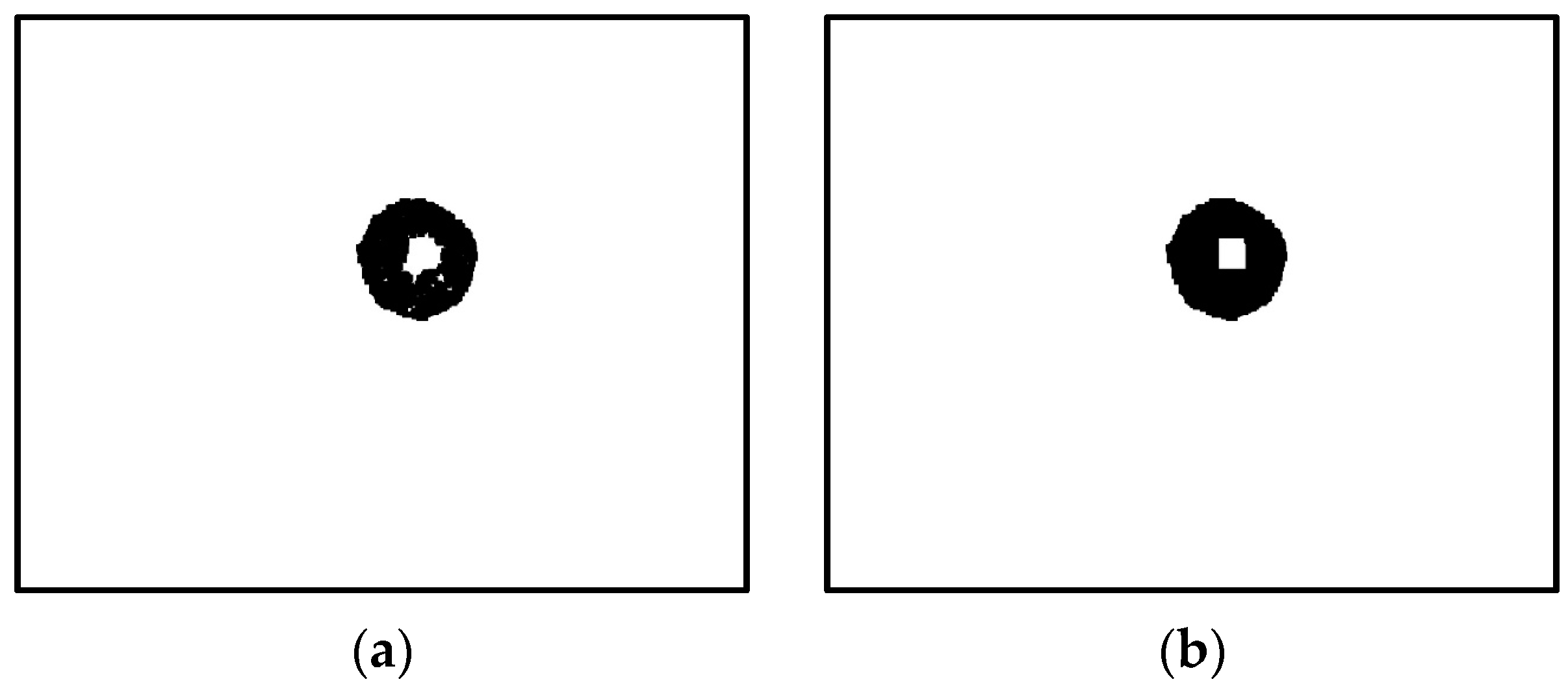
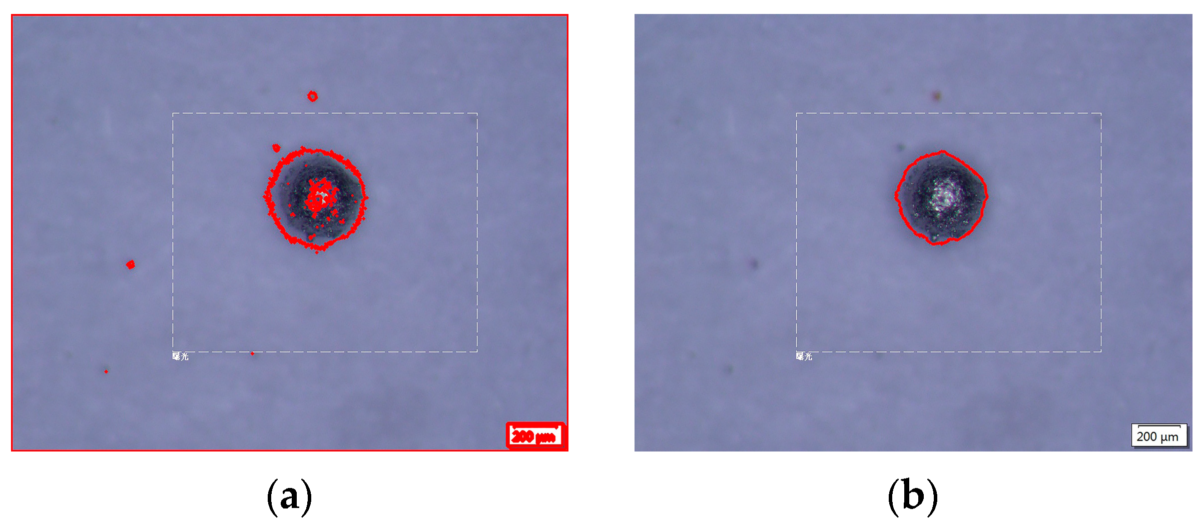
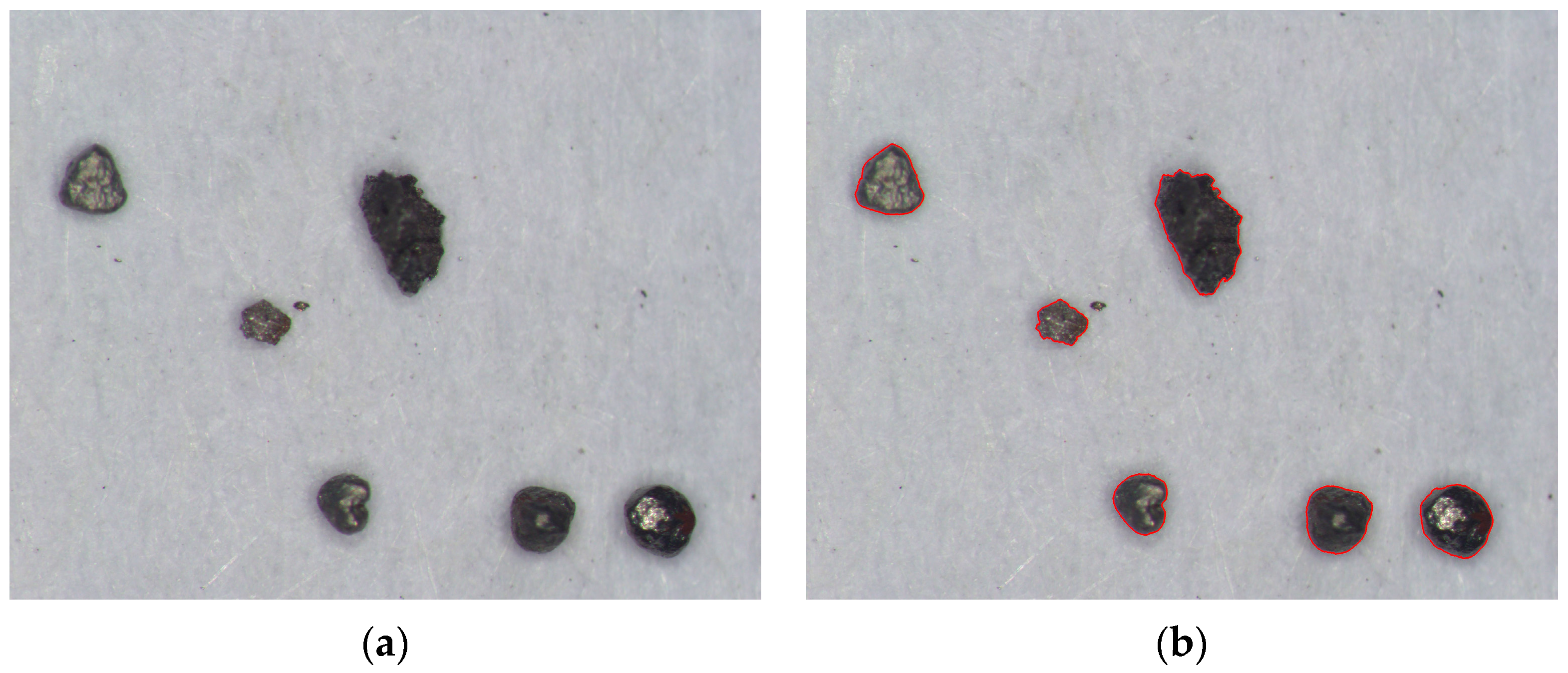
Finally, the Canny edge detection algorithm will output the extracted image contour. After utilizing the Canny edge detection algorithm on the morphologically processed image, the output image is shown in
Figure 9b. If the Canny edge detection algorithm directly extracts the contours without morphological processing, the result will be
Figure 9a. The extracted contours include contours with a large number of noise points.
The final contour extraction result is shown in
Figure 10, which shows that the algorithm can detect the contour of various particles.
2.3.2. Area, Perimeter and Result Analysis
After obtaining the contour of the oil particle through the Canny edge detection algorithm in OpenCV, the contourArea and arcLength functions can also be used to obtain the area and perimeter of the oil particle. The countArea function and arcLength function are mainly calculated by Green’s equation and arc length function [
27,
28]. The algorithm’s accuracy can be calculated by Equation (8).
where
is the accuracy of perimeter and area of the oil particles calculated by the algorithm and it is relative to the actual particle perimeter and area, i is the current oil particle number, K
L and K
A is perimeter and area of the oil particle, W
L, W
A is perimeter and area of the actual oil particles.
This paper extracts ten particle samples to measure the algorithm’s accuracy, as shown in
Table 1.
According to
Table 1, the algorithm’s accuracy in obtaining the perimeter and area of oil particles is about 95%, of which the reliability is high.
2.4. Oil Particle Shape Detection Based on Image Moment
Currently, in object shape detection, there are mainly two types: shape detection based on depth learning and shape detection based on traditional image recognition. Between them, deep learning is widely used in shape detection due to its advantages of comprehensive coverage and high accuracy. However, due to the data-driven characteristics of deep learning, its accuracy may be very low when its data set is relatively small, and the probability of false detection will significantly increase. In some cases where the data set is small, traditional image recognition techniques are often used to obtain better results.
There are many methods to detect the shape of objects through traditional image recognition methods, including corner detection, template matching, image moments, and other algorithms. These algorithms aim to obtain the target’s contour by the method described above.
Corner detection needs to calculate each pixel’s corner response function (CRF) value. It will judge whether the pixel is a local maximum. If so, it is determined as a corner. The shape of the target is simply detected by the number of corners. If the number of corners of the target is detected to be four, it is judged to be rectangular. If the number of corners of the target is detected to be three, it is determined to be a triangle; when the number of corners is higher than a certain threshold, it can be circular. The accuracy of this method is low, and it is difficult to identify its specific shape when facing an irregular target. False judgment easily occurs. Thus, this algorithm is unsuitable for detecting oil particles [
29,
30].
The template matching algorithm mainly obtains a coefficient matrix by traversing each pixel of the original image, then carrying out the correlation operations. The similarity between the template image and the original image can be compared through the parameter values in the coefficient matrix to obtain the results. The accuracy of the template matching algorithm is affected by the number of templates. If the target detected does not exist in the template library, it will lead to false judgment. As a consequence of the various shapes of particles in the oil, this method is also unsuitable for detecting oil particles [
31,
32].
The algorithm based on image moments can obtain feature parameters of each object shape by calculating the image moments in the image. Therefore, it can also extract the features of the irregular object for analysis without setting templates in advance, which reduces the labor cost. Moreover, the algorithm has high accuracy and fast operation efficiency, and the extracted feature parameters can also be used for other subsequent analyses. Hence, image moments were used to detect the object’s shape in this paper.
2.4.1. Obtain the Centroid through the First-Order Image Moment
Moment is a concept in statistics that can be regarded as an extension of the concepts of mean and variance. By considering the pixel coordinates of the image as two-dimensional random variables and the grayscale values as probabilities, we can apply the moments in statistics as image moments. Image moments include zeroth moment, first moment, second moment, Hu-moment, etc. The first-order moment is used to describe the image’s shape characteristics and the shape’s probability distribution. Therefore, this paper adopts the first-order and zeroth-order moments to realize the shape detection of oil particles. The first- and zero-order moments of the image and the centroid coordinates obtained from them can be calculated by equations [
33].
2.4.2. Polygon Fitting
The contour obtained after contour extraction has many corners. Although the approximate shape of the object itself is just a simple image, such as a sphere or a rectangle, due to the irregularity of the oil particles, the contour still has many corners. These uneven corners significantly affect the computer’s detection of object shapes, so it is necessary to fit the extracted contour into a polygon with only a few corners.
The Douglas–Peuckers algorithm is a special algorithm for polygon fitting. It takes a limited number of points from the digitized contour, turning them into a polyline, and to some extent, it can keep the original shape of the target. In this paper, the Douglas–Peucker algorithm was used to fit the extracted contour polygon. In this algorithm, the parameter epsilon (approximation precision of polygon fitting, which means the maximum distance between the original curve and the approximate curve) needs to be specially set. The smaller the value is, the more corner points are retained, and the greater the precision will be. The larger the value is, the smaller the number of corners remaining, and the smaller the precision will be.
The images corresponding to different
epsilon values are shown in
Figure 11.
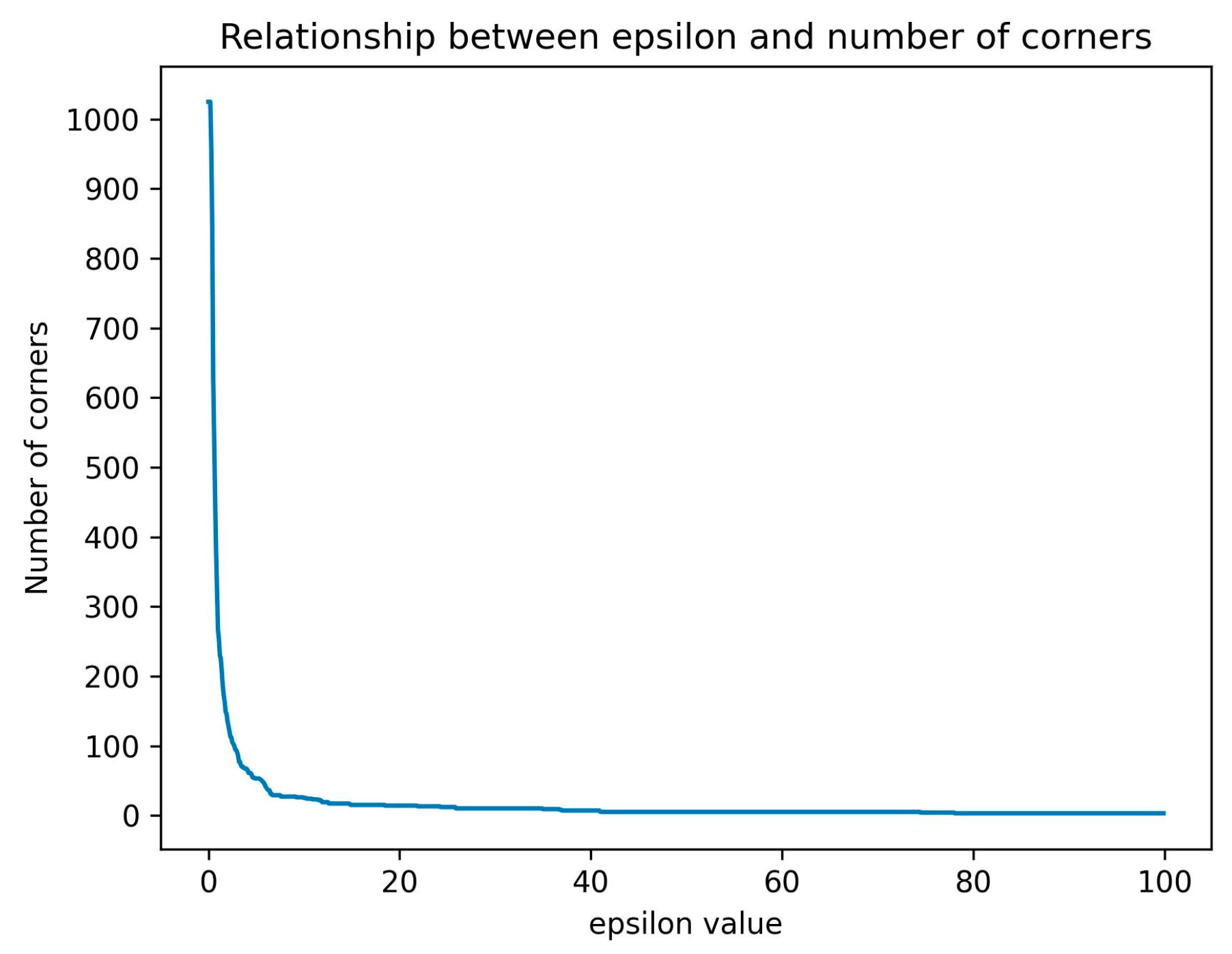
The relationship between epsilon and number of corners is shown in
Figure 12.
By comparing
Figure 11 and
Figure 12, it is not difficult to find that the contour with a smaller
epsilon has more corners than the big one. The polygonal fitting diagram retains the basic shape of the oil particles, which is convenient for subsequent analysis.
Thus, it can be seen that different targets should be set with corresponding epsilon, so this paper uses Equation (9) to set this value dynamically.
where
L is the circumference of the contour.
2.4.3. Shape Detection
After calculation of the centroid and polygonal fitting of the contour, the oil particle distance-angle can be drawn, where the x-axis is the size of the circumference angle centered on the centroid, and the y-axis is the distance from the circumference angle to the edge.
The angle and the distance from the circumference angle to the edge can be calculated by Equations (10) and (11).
where I
x and I
y is the ordinate and abscissa of the pixel point.
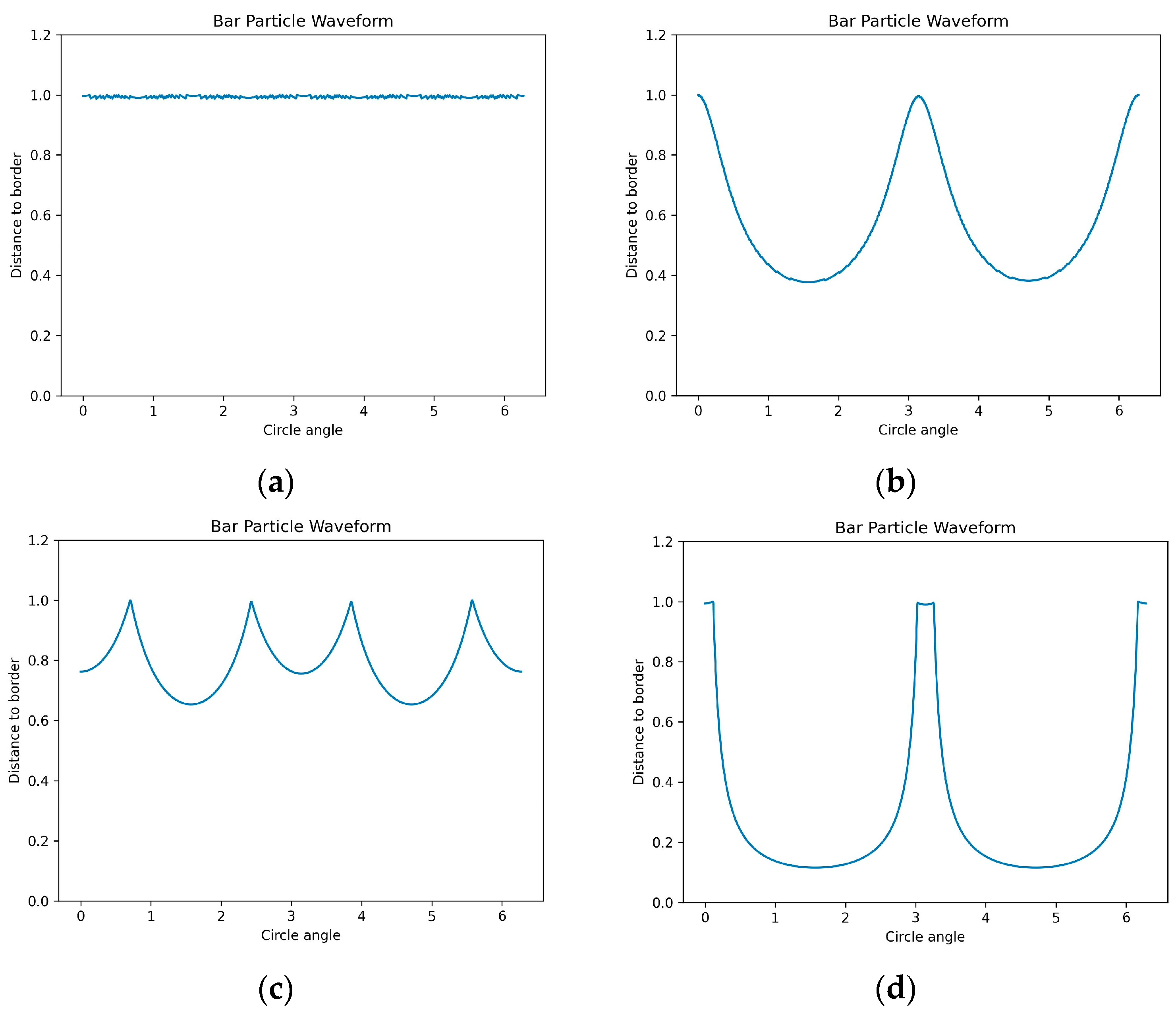
In
Figure 13, different particles’ waveforms have different shapes, so the following conclusions can be drawn:
- (1).
The waveform of the circle is a straight line, but because there is no perfect circle in nature, it is often presented in the form of an ellipse. The waveform of the ellipse has a certain degree of periodicity and appears in the form of a sine wave (as shown in
Figure 13a). The flattening degree of the ellipse is proportional to the fluctuation amplitude of the sine wave (as shown in
Figure 13b).
- (2).
The waveform of the polygon (excluding circle and ellipse) has many non-derivable points, and the number of non-derivable points is equal to the number of corners.
- (3).
The angle corresponding to the corner of the polygon is inversely proportional to the sharpness of the non-guided points (this means the D-value between the left derivative and the right derivative of the non-differentiable point value.)
- (4).
The waveform of the symmetric graph shows a high degree of symmetry and even periodicity.
According to
Figure 13, we can judge whether it is a spherical particle through the periodicity of the sine wave (since there is no perfect circle in nature, it can be considered that if the particle waveform has a large number of corners and is periodic, it can be identified as a spherical particle). The flattening degree is proportional to the fluctuation amplitude of the signal.
The main four unguided points of the blocky particles waveform are sharp and the four corners are periodic, as shown in
Figure 13c. In
Figure 13d, the four main unguided points of the strip particles waveform are similar to those of the blocky particles waveform, but the distance between one pair and the other is relatively long. The other particle waveforms can be regarded as irregular particles.
We could clearly analyze the waveforms of different particle shapes from the above.
2.4.4. Extracting Characteristic Parameters by Difference Operation
Although from
Figure 13 we can identify the particle shape of oil particles with our eyes, in order to detect oil particles in real time, an algorithm needs to be designed so that the computer can analyze the waveform. The most important parameters to identify the particle shape is the wave crest and wave trough in the waveform, so this paper used the difference method to extract the characteristic parameters in the waveform.
In the continuous domain, the first and second derivatives are generally used to judge the wave peaks and troughs in the waveform graph. The function needs to be fitted in the discrete domain before using the derivative method, but this method has defects. In order to achieve a high degree of fitting effect, the polynomial degree of fitting will be very high, which will cause the derivation process to become highly complex. Therefore, in the discrete domain, the difference method is often used to judge the wave peaks and troughs in the waveform.
The first-order difference method is to subtract two consecutive terms in the time series of the discrete waveform. The first-order difference operation is according to Equation (12).
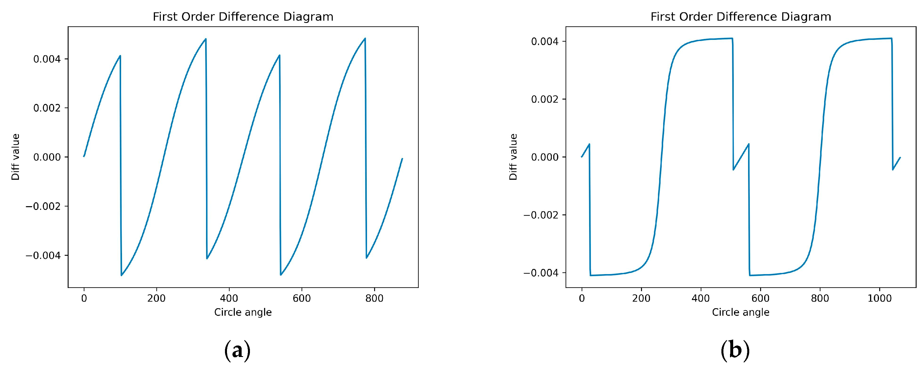
Figure 14 shows the results of blocky and strip particles after using the difference method.
Figure 14a is the first-order difference diagram of blocky particles, and
Figure 14b is the first-order difference diagram of strip particles.
According to
Figure 14, there are some step points, which are the number of corner points of the particle shape. As shown in
Figure 14, the number of corner points of the strip and rectangular particles is four. The degree of the step (the absolute of the highest point value minus the lowest point value) is the size of the angle. As shown in
Figure 14, the degrees of the four steps are almost equal because the corners of blocky particles and rectangular particles are both 90 degrees. The distance between two steps represents the length of the adjacent edge between two corner points. As shown in
Figure 14a, the distance between adjacent steps is almost equal, indicating that the particles tend to be blocky. In
Figure 14b, the distance between the first and second steps is far greater than that between the second and third steps, indicating that the particles tend to be strip-shaped particles.
In summary, this paper implements an algorithm to obtain the shape characteristics of the particles in the oil fluid in real time.
3. Conclusions
This research provides a new idea for the condition monitoring and fault diagnosis of ships and offshore engineering equipment, based on OpenCV. The designed method can be used in oil detection to achieve real-time detection of the circumference, area, and shape of particles in marine hydraulic oil. The accuracy can reach 95%.
In the field of using traditional image processing methods to detect oil particles, this paper not only uses the Canny edge detection algorithm to extract the particle contour, but also uses morphological processing to optimize the algorithm, and finally extracts the particle contour, perimeter and area. Furthermore, this paper also uses a method based on the image moment to successfully detect the specific shape of particles by analyzing the distance from the center of mass to the contour. Compared with other traditional image detection methods, this method can detect more specific characteristics of oil particles.
Compared with the deep learning algorithm currently used in a wide range, the advantage of the new method is that it does not require a massive training set and has high operation efficiency; for different circumstances, the depth learning algorithm needs to retrain. This algorithm only needs to adjust the corresponding parameters and has strong adaptability. There is no need to worry about the “overfitting” problem caused by the small amount of data in the depth learning algorithm.
Due to some disadvantages of the algorithm, we are considering combining it with the depth learning algorithm, in other words, using this algorithm to detect oil particles and the depth learning algorithm to classify oil particles. For example, in order to detect four types of oil particles with four shapes, if only the depth learning method is used, a total of 16 groups of data need to be prepared. Assuming that the data size of each group is 10,000, a total of 160,000 data sets is required. However, if the method in this paper is used to detect the shape and contour of particles, and deep learning is used to classify oil particles, only 40,000 data sets are needed, which is equivalent to reducing the amount of data by 75%. In general, this method can significantly reduce the training set required by the depth learning algorithm and improve the accuracy of the overall algorithm when the training set is not big enough. It is of great significance for the fault diagnosis of marine hydraulic systems.


 ,
, 


