4.1. Effects of Winds
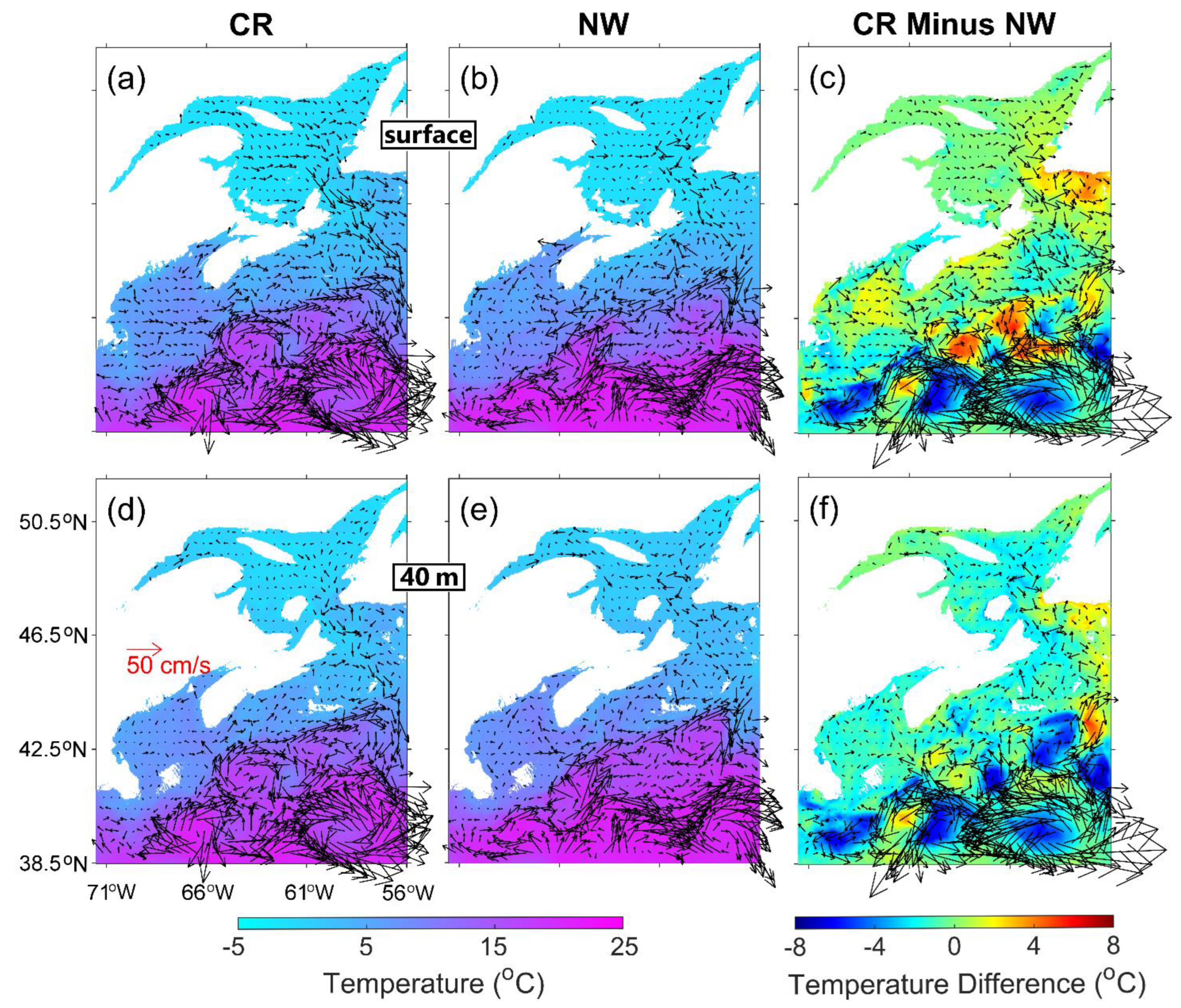
To examine the role of wind forcing over the GSL-ScS-GoM region and adjacent deep waters, the monthly-mean model results produced by submodel L2 in case CR are compared to their counterparts in case NW. Model results in February and August 2018 are chosen to represent the typical winter and summer months.
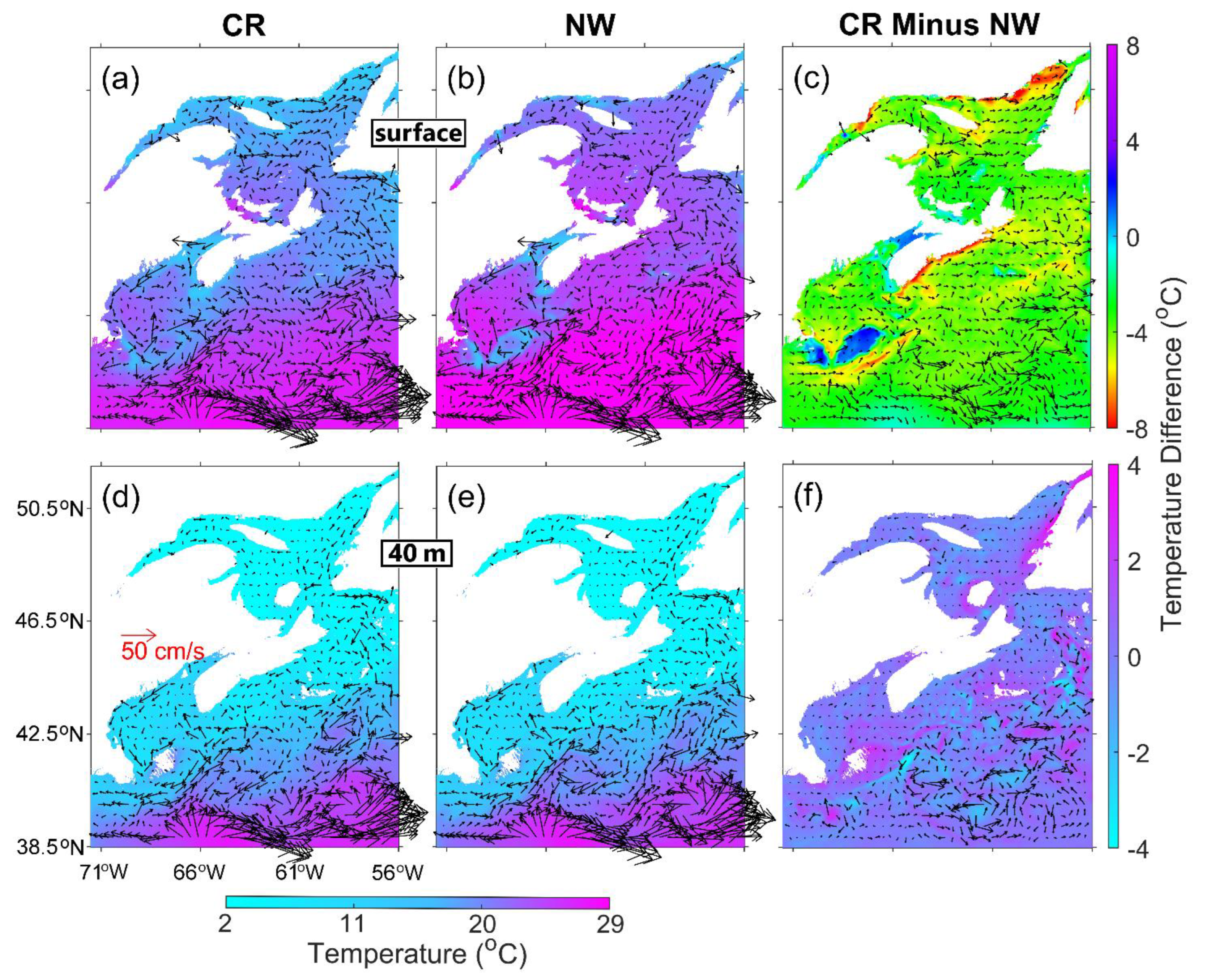
The February-mean SST (
;
Figure 8a) in 2018 has the typical horizontal distribution in the winter months, which is relatively cool and varies between −2 °C and 5 °C over the ScS, GSL, BoF, and southwestern NFS. Over the GoM and slope water region off the ScS,
varies between 5 °C and 15 °C. In the deep ocean waters to the south of the slope waters,
is warm and ranges between 15 °C and 21 °C. The February-mean surface circulation
also has many recognized features over the region, including the seaward surface currents over the southeastern GSL, spatially-varying currents on the ScS and GoM, the northeastward jet over the slope water region off the ScS, and the northern part of the Gulf Stream and associated eddies and meanders in the deep waters to the south of the slope water region (
Figure 8a). Both
and
in this month also have small-scale features associated with the warm- and cold-core rings, thermal fronts, and the meandering of the slope water jet over the slope waters and adjacent deep ocean waters off the ScS-GoM.
The February-mean sub-surface (40 m) temperature and currents
and
;
Figure 8d) in 2018 have large-scale horizontal features highly similar to their counterparts at the sea surface in case CR (
Figure 8a), except for the weaker current magnitudes at 40 m. The weak vertical stratification in the top 40 m over the L2 domain in winter months results from both the winter convection and intense wind-induced vertical mixing. Winter convection is referred to as the sinking process of cold surface waters to deeper depths due to the largely negative net heat flux at the sea surface (i.e., the ocean water losses heat to the air) in the late fall and winter months, which is one of the important processes over the ECS. The Nova Scotia Current [
42], which is a southwestward coastal jet over the inner shelf of the ScS, is approximately compensated by the northeastward wind-driven currents in the surface mixed layer in February 2018.
The February-mean SST (
;
Figure 8b) in 2018 in case NW is very similar to, and slightly cooler than, the counterpart in case CR over the coastal and shelf waters, including the GSL, ScS, and GoM. In the slope waters and adjacent deep ocean waters off the ScS-GOM, the February-mean SST in case NW, particularly the small-scale SST features associated with eddies and meanders, significantly differs from the counterpart in case CR. The February-mean surface currents in case NW (
;
Figure 8b) also significantly differ from the counterparts in case CR, particularly in the slope and adjacent deep ocean water regions. This indicates the importance of the wind forcing in surface currents and SST in the winter months over the L2 domain in case CR.
The monthly-mean sub-surface (40 m) temperature and currents in case NW (
,
;
Figure 8e) are highly similar to the counterparts at the sea surface (
and
;
Figure 8b) in February 2018, indicating that the vertical stratification of hydrography in this month is very weak in the top 40 m in case NW due to the winter convection mentioned above. The February-mean fields of (
,
) in 2018 in case NW differ from the counterparts in case CR over the slope waters and beyond, indicating the important role of wind forcing on the sub-surface currents. It should be noted that the large February-mean currents in case NW (
Figure 8b,e) are driven by the baroclinic dynamics, nonlinear tidal processes, and boundary forcing, since wind forcing is excluded in this case.
The differences in the monthly-mean model results between cases CR and NW are used to quantify the accumulative effect of wind forcing on the 3D circulation and hydrography. Over much of the coastal and shelf waters in the L2 domain, the differences in the February-mean SST between cases CR and NW (
;
Figure 8c) are positive and up to 3 °C. The differences in the February-mean sub-surface (40 m) temperature between the two cases (
;
Figure 8f) are mostly negative and up to −2 °C over the coastal and shelf region. Over the seCS, the vertical stratification in the surface mixed layer is weak in winter mainly due to strong winter convection. The wind-induced vertical mixing further blends the relatively warm subsurface waters with the relatively cool surface waters in the surface mixed layer. This explains why the wind forcing makes the SST warmer and sub-surface temperature cooler, as shown in
Figure 8c,f. The monthly-mean current differences between these two cases at the sea surface (
;
Figure 8c) and 40 m (
;
Figure 8f) over the coastal and shelf waters represent the currents directly and indirectly driven by winds in the winter months.
Over several coastal areas of the L2 domain, such as the BoF, GeB, and the inner shelf off Yarmouth, the tidal forcing is very strong, resulting in particularly weak vertical stratification of hydrography in February 2018. As a result, sensible and latent heat fluxes play important roles in affecting the February-mean SST than the wind-induced vertical mixing over these areas, with negative
of about −2 °C in February 2018 (
Figure 8c).
Over the slope waters and deep ocean waters off the ScS-GoM, there are significantly large differences in the February-mean temperature and currents between cases CR and NW (
Figure 8c,f). In addition to the effect of wind-induced mixing and currents mentioned above, these large differences are generated by the wind-induced modulation of large-scale circulation (i.e., the Gulf Stream), warm/cold-core rings, and thermal fronts in case CR. The effect of wind forcing on currents can be categorized into direct and indirect types. The direct effects of wind forcing include the wind-driven currents and shelf waves excited by winds. The indirect effects include density-driven currents that are ultimately driven by winds, as well as wind-induced modulations of nonlinear circulation features, such as eddies, rings, and frontal structures. In the winter months, the wind forcing over the seCS is typically strong, and thus significantly modifies the nonlinear features of the hydrography and circulation over the slope water region and adjacent deep waters. The modulation of hydrography, in return, modifies density-driven currents and baroclinic hydrodynamics. As a result, the simulated Gulf Stream in case NW shows significantly different circulation features and eddies/meanders from their counterparts in case CR. These large current differences are associated mainly with wind-induced modulations of large-scale circulation, rather than the wind-driven currents. In addition, the wind forcing modifies the locations and intensities of warm-core rings pinched off from the northern side of the Gulf Stream. As mentioned earlier, the warm-core rings are clockwise and measured about 1 km vertically [
34]. As a result, the differences between cases CR and NW in terms of monthly-mean temperatures in February 2018 are positive (negative) over clockwise (counterclockwise) circulation differences, as shown in
Figure 8c,f.
In contrast to the weak vertical stratification in the surface mixed layer in winter, strong thermal stratification occurs at the bottom of the thin surface mixed layer in summer over the seCS, mostly due to the large surface heating and relatively weak wind-induced vertical mixing in late spring and summer [
43]. The thickness of the surface mixed layer (about 10 m) in the summer months is also much thinner than its counterpart (about 50 m) in the winter months [
44].
The monthly-mean SST (
;
Figure 9a) in August 2018 in case CR also has typical horizontal distribution in summer months, which is moderately warm and ranges between 10 °C and 20 °C over the northern GSL, BoF, and southwestern NFS, and between 14 °C and 21 °C over the central ScS. Over the central and western GoM, the slope water region off the ScS, and coastal waters off PEI,
is warmer and ranges between 20 °C and 25 °C in this month in case CR. Over deep waters off the ScS-GoM,
is warmest and ranges between 25 °C and 27 °C in this month (
Figure 9a). It should be noted that
is relatively cool over the BoF, GeB, and coastal waters off Yarmouth in this month, mainly due to strong tidal mixing and tidal rectification. The relatively cool monthly-mean SST over the inner ScS in August 2018 in case CR (
Figure 9a) indicates coastal upwelling driven by winds in summer.
The August-mean surface currents (
;
Figure 9a) in 2018 in case CR have many well-known large-scale surface circulation features, including the southeastward outflow associated with the seaward spreading of the freshwater discharge from the SLR over the southeastern GSL, the relatively intense southwestward flow along the coast of the western GoM, and the strong flow, eddies, and meanders associated with the Gulf Stream in the slope waters and adjacent deep ocean waters. In this month,
is southeastward (seaward) over the southwestern GSL, and northeastward over the eastern GSL, except for coastal waters off western Newfoundland. Both
and
in August 2018 also show fine-scale features of circulation and SST associated with the local tidal mixing/advection and topographic steering over GeB (e.g., the anticyclonic circulation along isobaths around GeB) and adjacent (
Figure 9a).
Due to strong thermal stratification at the bottom of the thin surface mixed layer resulting from the positive surface heat fluxes in summer, the August-mean sub-surface (40 m) temperature
significantly differs from the August-mean SST (
. In this month,
in case CR (
Figure 9d) is relatively cool, ranging between 2 °C and 4 °C over the GSL, northeastern ScS, and southwestern NFS. Over the eastern GoM and swScS,
is about 10 °C. Over the BoF, southern GoM, and slope waters off the ScS-GoM,
ranges between 10 °C and 20 °C. In deep ocean waters to the south of the slope waters,
is significantly warmer and ranges between 20 °C and 26 °C.
In the GoM and over the slope waters and adjacent deep ocean waters off the ScS-GoM, the monthly-mean sub-surface (40 m) currents (
;
Figure 9d) have large-scale circulation features similar to their counterparts at the sea surface (
;
Figure 9a) in August 2018 in case CR. Over these regions, the August-mean sub-surface circulation in case CR (
Figure 9d) features the large-scale cyclonic coastal currents in the GoM, the slope water jet, the northern part of the Gulf Stream, and associated eddies and meanders at 40 m. In the GSL and ScS, by comparison, the August-mean sub-surface (40 m) currents significantly differ from their counterparts at the sea surface, mainly due to the strong vertical stratification of hydrography at the bottom of the thin surface mixed layer in the summer months. In the GSL, the August-mean sub-surface currents in case CR are very weak over the southwestern region, and have an anticyclonic recirculation over the eastern region with a narrow southwestward jet along the coast of eastern Newfoundland (
Figure 9d). Over the inner ScS, the Nova Scotia Current is much more well-defined at 40 m than at the sea surface (
Figure 9a,d) in the summer months.
Without wind forcing in case NW, the simulated August-mean SST (
;
Figure 9b) in 2018 is relatively warm and about 24 °C in the GSL, except for several coastal waters over the northern GSL. Over the ScS and GoM,
in this month varies between 24 °C and 27 °C, except for relatively low SST over coastal and shallow areas with strong tidal mixing/advection in the GoM, including the GeB and BoF. In the slope waters and deep ocean waters,
in this month is warm and varies between 27 °C and 29 °C (
Figure 9b). Without wind-inducing vertical mixing,
is warmer than
in August 2018 over the whole L2 domain, except for areas affected significantly by tidal mixing/advection in the GoM. In case NW, the thermal energy gained from the positive net heat flux at the sea surface (shortwave and longwave radiations) is trapped in the unrealistically thin surface mixed layer in summer due to the absence of wind-induced vertical mixing.
The August-mean surface currents (
;
Figure 9b) in case NW have large-scale features similar to their counterparts in case CR (
;
Figure 9a), particularly in the deep ocean waters off the ScS-GoM. Noticeable differences, however, occur between
and
over coastal and shelf waters in August 2018. Without wind forcing,
is seaward as part of the estuarine plume over the southwestern GSL, but is approximately southwestward over the eastern GSL in case NW. The simulated Nova Scotia Current over the inner shelf of the ScS in case NW is unrealistically too strong at the sea surface (
Figure 9b) due to the lack of wind forcing in this case.
The large-scale features of the August-mean
and
in case NW (
Figure 9e) are highly comparable to their counterparts in case CR (
Figure 9d). This indicates that, in summer months, wind forcing is usually weak and does not significantly affect the sub-surface (15 m or deeper) circulation and hydrography, except for coastal waters during upwelling- and/or downwelling-favorable wind events.
Figure 9c presents differences in the monthly-mean SST (
) and surface currents (
) between cases CR and NW in August 2018. The values of
are negative over the L2 domain with the maximum negative value of about −7 °C, except for some local areas affected by strong tidal mixing/advection. This indicates the important role of wind-induced vertical mixing for transferring thermal energy from the sea surface downward. Without wind-induced vertical mixing (case NW), the thermal energy gained from positive surface heat fluxes (shortwave and longwave radiations) is trapped in the very thin surface mixed layer, resulting in unrealistically too warm SSTs in case NW. Positive values of
occur over several local areas, including the BoF and GeB (
Figure 8c). Over these areas, wind-induced horizontal mixing and advection, as well as the positive net heat flux associated with wind stress (latent and sensible heat fluxes), in case CR significantly counteract the SST cooling generated by the strong tides.
The magnitudes of
in August 2018 (
Figure 9c) are relatively small at about 0.1 m s
−1 over the ScS and GoM, and up to 0.2 m s
−1 in the western GSL. Large magnitudes of
also occur over the slope waters off the ScS-GoM. The relatively small magnitudes of
over the coastal and shelf waters in this month demonstrate the direct effect of wind forcing on the summertime surface circulation. In contrast, the relatively large magnitudes of
over the slope waters and in the western GSL are mainly associated with the wind-induced modulations of meanders and eddies. The magnitudes of
over the slope waters and adjacent deep ocean waters in August 2018 (
Figure 9c) are significantly smaller than their counterparts in February 2018 (
Figure 8c), indicating that the wind forcing and wind-induced modulations of large-scale circulation are generally much weaker and smaller in the summer than in the winter.
Figure 9f demonstrates that, in August 2018,
is positive over the L2 domain, except for several patches with negative values over the slope waters off the ScS-GoM. The positive values of
indicate that subsurface waters are cooler in case NW than in case CR in this month. This can be explained by the fact that the incoming heat fluxes at the sea surface could not easily penetrate downward without wind-induced vertical mixing (case NW) in the summer months. There are many small-scale features with noticeable negative values of
over the slope waters and deep ocean waters off the ScS-GoM (
Figure 9f), indicating the modulation effect of wind forcing on mesoscale eddies and recirculation over these regions. There are also several small-size patches and narrow strips of negative values of
(~−1 °C) over coastal and shelf waters (
Figure 9f), such as the western ScS, associated with wind-induced modulation of small-scale nonlinear dynamics.
The magnitudes of
in August 2018 (
Figure 9f) are relatively small over coastal and shelf waters in the L2 domain, due to the fact that winds are generally weak in August and the direct effect of wind forcing on the 3D circulation mainly occurs in the top 10 m. Over slope waters and deep ocean waters off the ScS-GOM, by comparison, the values of
in this month are relatively large, which are mainly associated with the wind-induced modulation in the locations and intensities of meanders and warm/cold-core eddies.
The accumulative effect of winds on the monthly-mean salinity fields in the two months is examined next based on model results in cases CR and NW. In February 2018, the monthly-mean SSS (
;
Figure 10a) in case CR is relatively low and ranges between 27 and 32 (psu) over the SLE, southern GSL, and inner shelf of the ScS (
Figure 10a). Over the GoM,
is typically about 33. Over the slope waters off the ScS-GoM,
ranges between 32 and 35. In the deep ocean waters to the south of the slope waters,
is high and generally above 35. In this month,
also has some fine-scale features associated with salinity fronts and nonlinear circulation.
The February-mean sub-surface (40 m) salinity (
;
Figure 10d) in 2018 has a horizontal distribution very similar to
(
Figure 10a), except for the relatively higher values at 40 m over the SLE, southern GSL, and the inner shelf of the ScS. The high similarity between
and
in this month is mainly due to winter convection and the strong wind-induced vertical mixing in winter. It should be noted that a sharp salinity front approximately follows along the shelf break of the ScS-GoM (
Figure 10a,d), which forms an important frontal boundary separating the relatively cool and fresh shelf waters from the warm and salty slope and deep ocean waters [
45].
Without wind forcing in case NW, the February-mean SSS (;
Figure 10b) in 2018 is lower than the counterpart in case CR (
Figure 10a) over the eastern GSL, southwestern NFS, ScS, eastern GoM, and coastal waters near river mouths in the northern GSL and western GoM. This indicates the important effect of wind-induced mixing on the salinity distribution in the surface mixed layer and seaward spreading of low-salinity waters over the southwestern GSL and eastern and inner ScS in the winter months. These low-salinity waters are associated with the seaward (equatorward) spreading of estuarine waters from the SLE [
41]. Without wind-induced vertical mixing (case NW), the low-salinity waters are unrealistically trapped within the very thin surface layer. Strong winds in this month also modify the salinity distributions over the slope waters and adjacent deep waters through wind-induced modulations of baroclinic dynamics and nonlinear circulation features in the upper water columns.
Over the coastal and shelf waters of the L2 domain, the monthly-mean sub-surface (40 m) salinity (
;
Figure 10e) in February 2018 in case NW has large-scale features highly similar to the counterpart in case CR (
;
Figure 10d), due to the winter convection. Significantly large differences between
and
occur over the slope waters and deep ocean waters off the ScS-GoM, mainly due to the large modulation effect of wind forcing on mesoscale eddies and warm/cold-core rings over these regions. A sharp salinity front also occurs at the shelf break of the ScS-GoM in this month in case NW.
Figure 10c presents the differences in February-mean SSS in 2018 between cases CR and NW (
). The salinity differences are significantly positive over the southwestern NFS, inner and middle ScS, and coastal waters of the GoM, with the maximum positive value of about 4. Due to the important effect of wind forcing on large-scale circulation and associated eddies and meanders over the slope waters and adjacent deep ocean waters off the ScS-GoM, large negative (positive) values of
are associated with cyclonic (anticyclonic) rings of
(
Figure 10c) in February 2018.
At 40 m, due to winter convection, the monthly-mean sub-surface salinity differences between cases CR and NW (
;
Figure 10f) in February 2018 are relatively small in the GSL, ScS, and GoM, except for some coastal areas due to the local wind effects. In the slope waters and adjacent deep ocean waters,
is relatively large, with large negative (positive) values associated with the cyclonic (anti-cyclonic) currents of
, mainly due to the modulation effect of wind forcing as mentioned above.
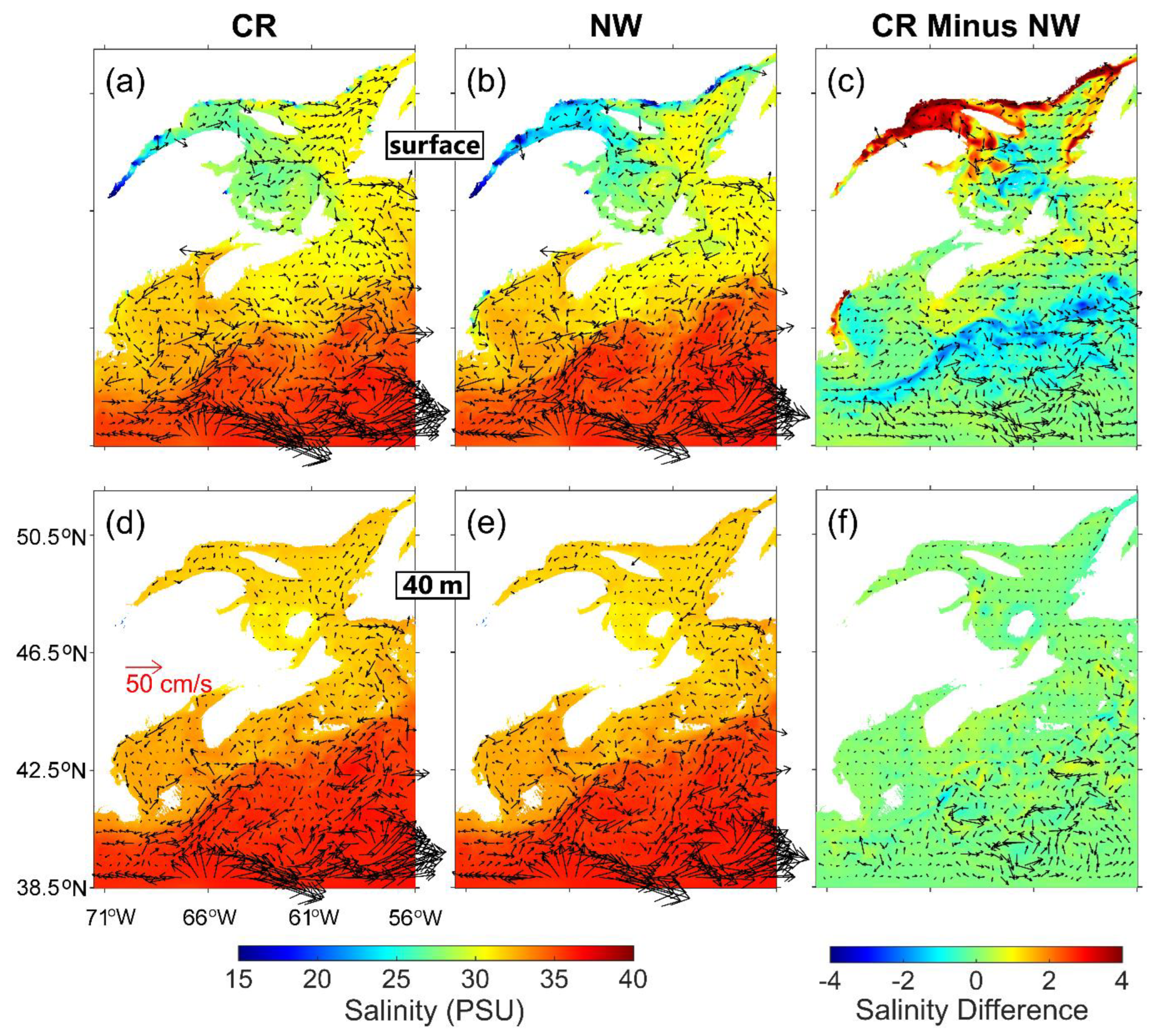
In August 2018, the monthly-mean SSS (
;
Figure 11a) is relatively low and ranges between 26 and 29 over the western GSL and coastal waters off CBI. The relatively low
over these areas is due mainly to the large discharge from the SLR during the spring and subsequent propagation of the low-salinity estuarine plume. Over the eastern GSL, southwestern NFS, GoM, and coastal waters of the ScS (except for coastal waters off CBI),
generally ranges from 30 to 32. Over the slope water region of the ScS,
ranges from 31 to 34. Over the deep ocean waters off the ScS-GoM,
is generally above 35. There are some fine-scale SSS features of
associated with salinity fronts and nonlinear circulation over the GSL, GoM, slope waters of the ScS-GoM, and adjacent deep ocean waters. A salinity front occurs at the shelf break of the ScS-GoM.
Since wind-induced vertical mixing is generally weak in summer, the August-mean sub-surface (40 m) salinity (
;
Figure 11d) in case CR differs from the counterpart at the sea surface (
Figure 11a). Over the GSL, ScS and GoM,
in this month is nearly uniform and varies between 32 and 33, with a well-defined salinity front at the shelf break of the ScS and GoM. In the slope waters and adjacent deep ocean waters off the ScS-GoM,
in this month is high and varies between 35 and 37.
The August-mean SSS (
;
Figure 11b) in case NW is relatively low and varies between 22 and 28 over the western GSL and coastal waters around CBI. This can be explained by the fact that, without wind forcing, freshwater discharge from the SLR remains in the thin surface layer for a long time and spreads seaward. In this month,
is nearly uniform and ~32 in the GoM, and between 30 and 32 over the central and southwestern ScS. At the shelf break of the ScS-GoM,
in this month has a well-defined frontal boundary, with high
over 35 in the offshore waters beyond the shelf break.
The August-mean sub-surface (40 m) salinity (
;
Figure 11e) in case NW in 2018 is horizontally uniform and ~33 over shelf regions of the GSL, ScS, and GoM, and relatively high of over 35 in the slope waters and adjacent deep ocean waters. There is a sharp salinity front at the shelf break (
Figure 11e).
The differences in the August-mean SSS (
;
Figure 11c) between cases CR and NW are significantly positive and about 4 over the northwestern GSL and inshore waters of the northern GSL, which indicates the important role of wind forcing in blending the low-salinity surface waters with high-salinity sub-surface waters over these areas. Over the ScS, GoM, and deep ocean waters,
is also positive but small, about 1. Over the slope waters of the ScS-GoM,
is mostly negative. By comparison, the differences in the August-mean sub-surface salinity (
;
Figure 11f) between cases CR and NW are relatively small over the whole L2 domain, particularly over the shelf regions.
Over the slope water region off the ScS-GoM,
in August 2018 features a noticeable negative-value zone (
Figure 11c). To further demonstrate the role of wind forcing in generating the negative values of
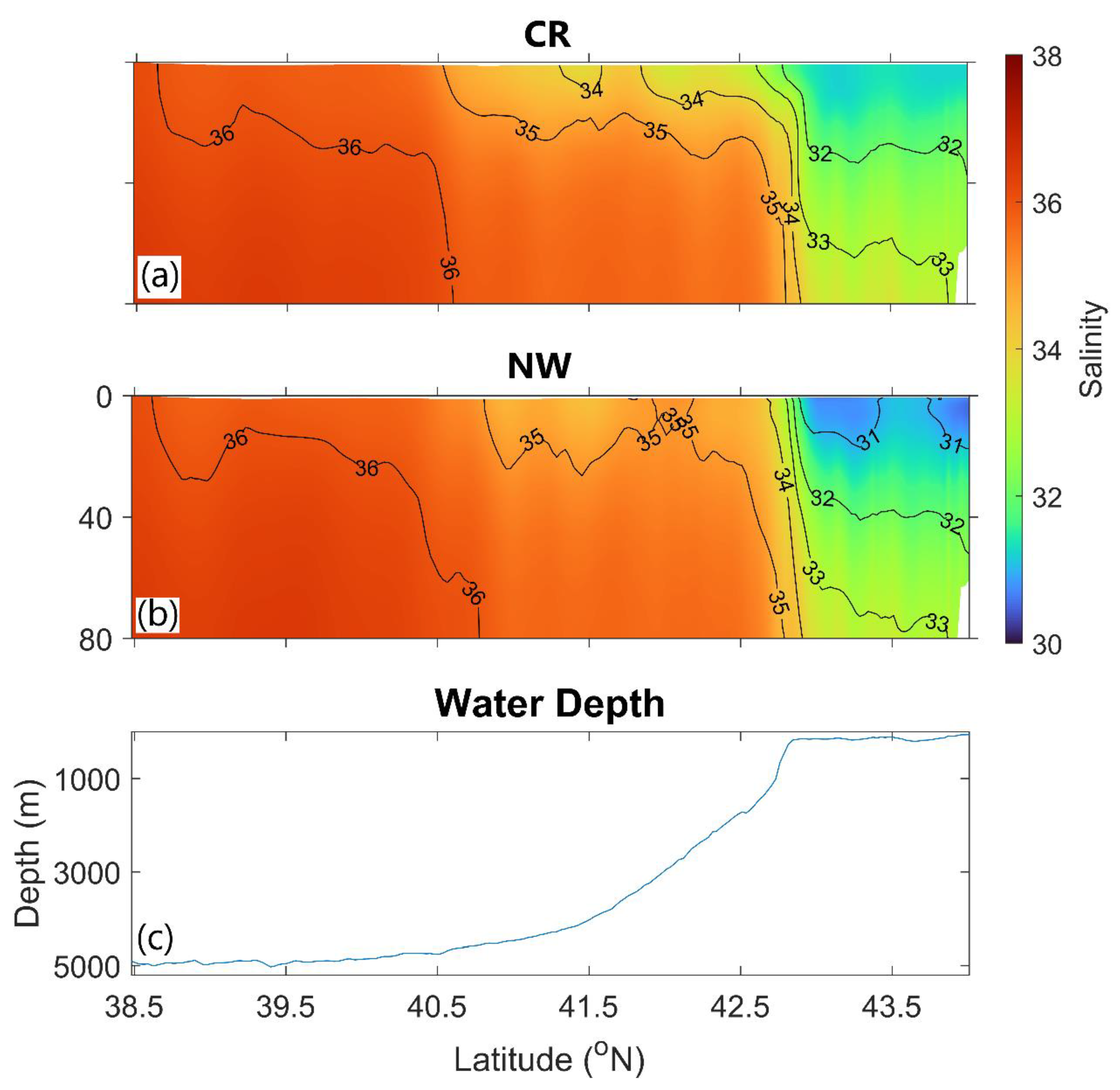
over this slope region, we examine the August-mean salinity in cases CR (
) and NW (
) along transect PQ (marked in
Figure 1b), which is a cross-shelf transect over the swScS. Distributions of
and
in the top 80 m along transect PQ in August 2018 are shown in
Figure 12a,b. The salinity front in the top 20 m is broader over the slope portion of the transect (between 41.5 ° N and 42.8° N;
Figure 12c) in case CR than in case NW (
Figure 12a,b), which is mainly due to the effect of wind forcing on the seaward transport of coastal waters in case CR. As a result,
(
Figure 12a) is lower than
(
Figure 12b) over the slope region of transect PQ in August 2018. For the same reason, negative values of
also occur over other slope waters to the south of the ScS and GoM in the summer months (
Figure 11c).
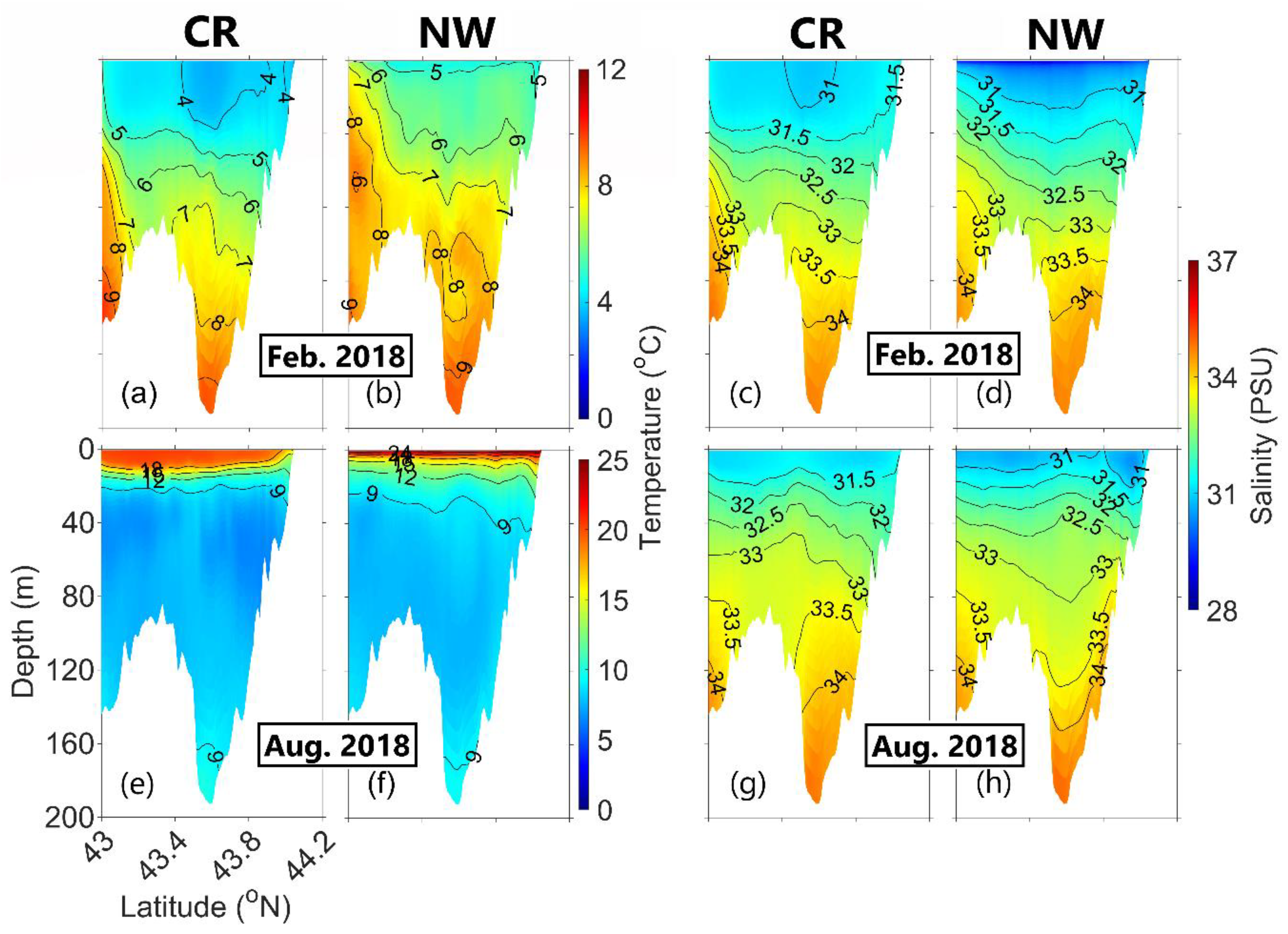
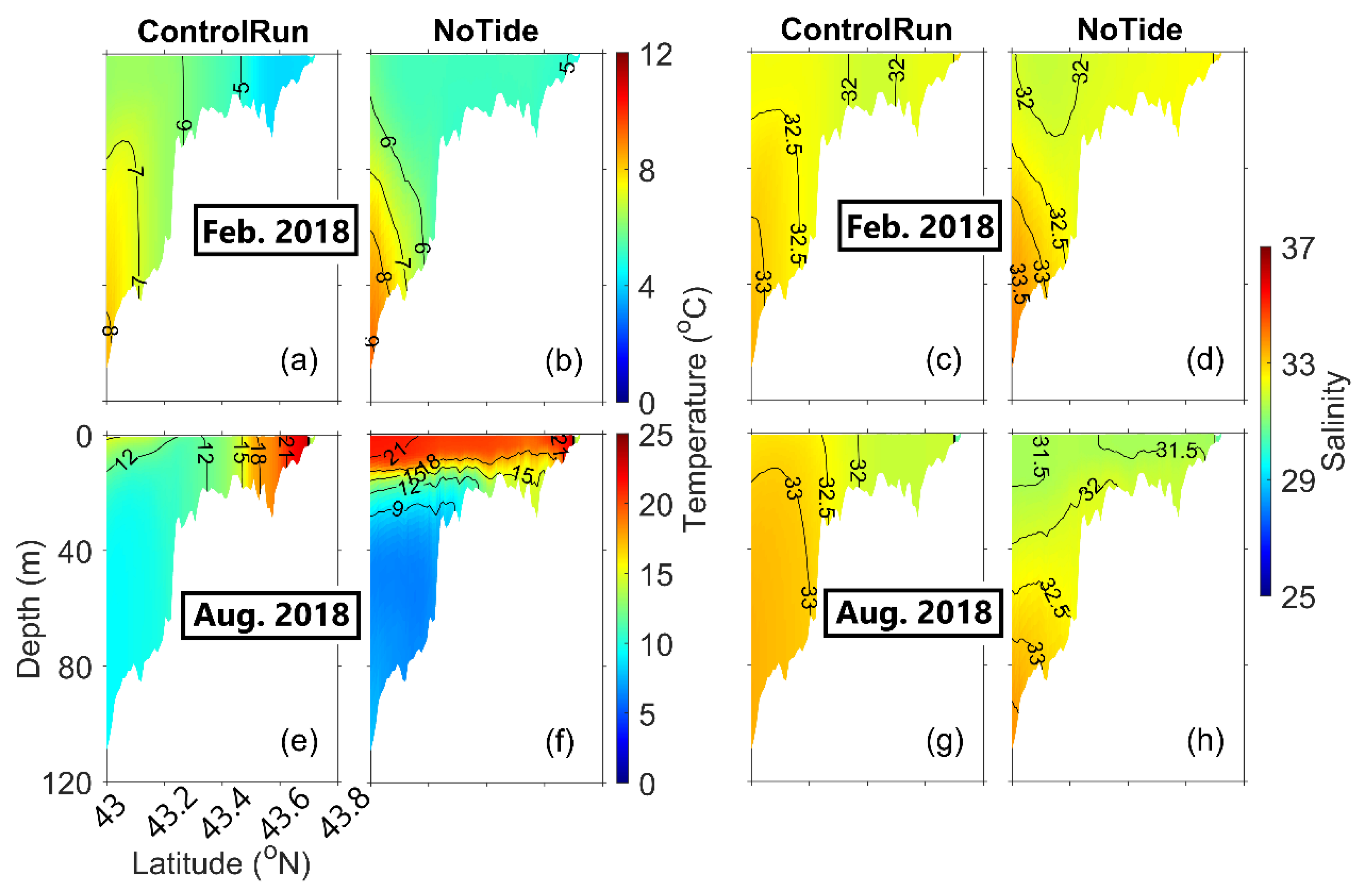
Vertical profiles of the monthly-mean temperature and salinity in February and August 2018 on transect PP’ (
Figure 1c) produced by submodel L3 in cases CR and NW (
,
,
,
) are analyzed to examine the role of winds in the vertical stratification over the swScS. In February 2018, both
and
(
Figure 13a,c) have a three-layer vertical structure with a cold (<5 °C) and fresh (<32) surface layer in the top ~40 m, a relatively warmer (between 5 °C and 7 °C) and saltier (between 32 and 33) intermediate layer at depths between 40 m and 100 m, and a warm (>7 °C) and salty (>33.5) bottom layer at depths below 100 m. As mentioned earlier, strong winter convection is responsible for the nearly uniform vertical stratification in the surface mixed layer in this month in case CR (also reduces the upper-column vertical stratification in case NW). Wang et al. [
9] demonstrated that the Nova Scotia Current splits into two branches over the northern flank of LaHave Basin: a narrow inshore branch (southwestward) over the inner shelf of the swScS and a broad offshore branch (meandering southward) over the western portion of LaHave Basin. The offshore branch of the Nova Scotia Current transports relatively cool and low-salinity upper-column waters seaward and crosses transect PP’ at the middle, resulting in the relatively cool (~4 °C) and low-salinity (~31) waters in the top ~40 m in the middle section of the transect.
In case NW, by comparison, the vertical stratification of
and
(
Figure 13b,d) in the top ~40 m in February 2018 is noticeably stronger than the counterpart in case CR, indicating the important role of wind-induced vertical mixing. In additional to vertical mixing, winds also affect the hydrography over the swScS through wind-induced modulation of circulation. Both
and
(
Figure 8c,f) are northeastward in the inner ScS, and strong and offshore over the western portion of LaHave Basin. This implies the modulation effect of winds on the Nova Scotia Current in February 2018 counteract the inshore branch and enhance the offshore branch of the Nova Scotia Current, which also contributes to the differences between
and
and between
and
in this month.
In August 2018,
and
in case CR (
Figure 13e,g) show a three-layer vertical structure, consisting of a warm (>18 °C) and fresh (<31.5) surface layer in the top ~10 m, a relatively cool (~6 °C) and fresh (between 32 and 33) intermediate layer between 20 m and 80 m, and a warmer (between 8 °C and 9 °C) and saltier (>33) bottom layer below 80 m. This three-layer structure of hydrography is normally well-established between the late spring and early autumn [
1]. The August-mean thermocline along transect PP’ in case CR is nearly horizontal and at depths of about 10 m over the middle shelf of the transect (beyond ~50 km away from the coast), tilts up over the inner shelf, and reaches the surface near the coast (
Figure 13e). The tilts of the August-mean thermocline and 31.5-salinity layer over the inner shelf in case CR (
Figure 13e,g) are associated by coastal upwelling induced by upwelling-favorable (northeastward) winds in the summer months.
The August-mean thermohaline on transect PP’ in case NW is unrealistically too shallow over the middle of the transect (
Figure 13f), due to the absence of wind-induced vertical mixing. Furthermore, the August-mean thermohaline in case NW does not tilt up over the inner shelf due to the absence of wind-induced upwelling. Below 30 m,
and
(
Figure 13f,h) also have vertical distributions considerably different from the counterparts in case CR (
Figure 13e,g) in August 2018. These differences (below 30 m, in August 2018) are partially associated with wind-induced modulation of baroclinic hydrodynamics. The shelf waves excited by winds in submodel L2 are present in case CR, but absent in case NW, also contributing to the differences between
and
and between
and
in August 2018.
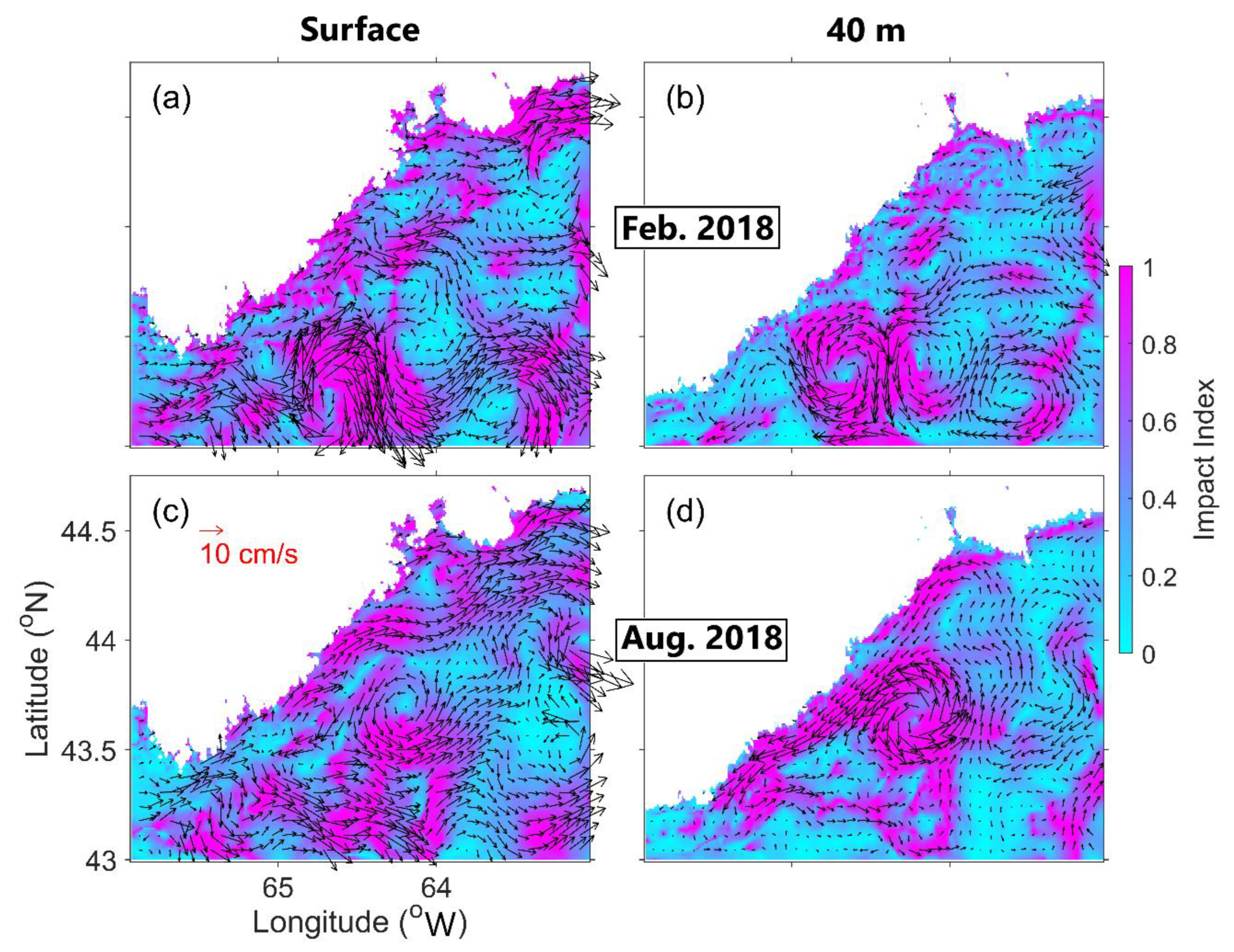
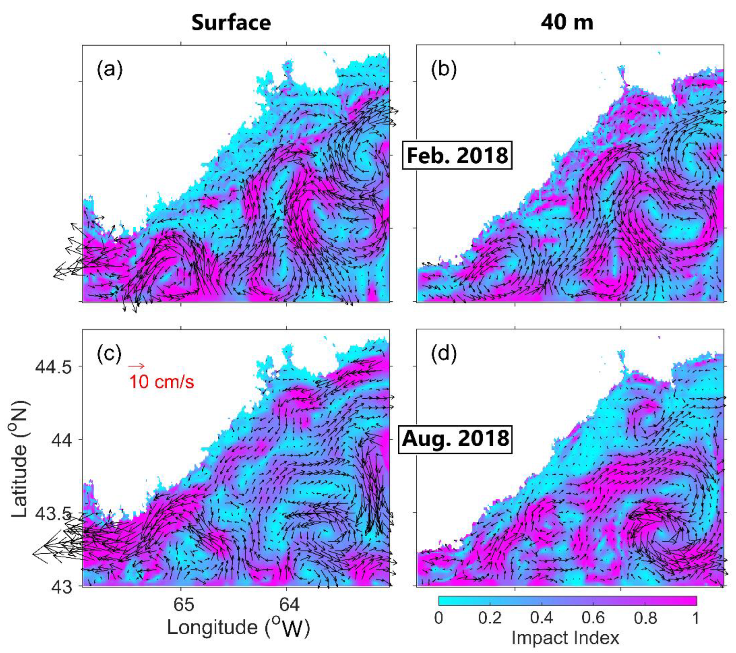
To quantify the effects of winds on the monthly-mean currents over the swScS, we calculate the impact index (
) of wind forcing at depth
(
equals 0 and 40 at the sea surface and the subsurface of 40 m, respectively) based on the L3 model results using the method by Wang et al. [
9].
In February 2018, the values of
(
Figure 14a) are large in the inner swScS mainly due to the northeastward wind-driven currents. The large values of
in the middle shelf are mainly associated with the wind-induced modulation of nonlinear circulation features, with contributions from wind-driven currents (e.g., eastward
in the southwestern and southeastern portions of the swScS). In this month, the values of sub-surface (40 m) impact index (
;
Figure 14b) are highly comparable to their counterparts at the sea surface (
;
Figure 14a), except for the relatively smaller magnitudes at the sub-surface (40 m) than at the sea surface. The high similarities between
and
in February 2018 can be mainly explained by the strong vertical mixing and weak vertical stratification over the swScS in winter.
In August 2018, the wind-driven currents are northeastward and oppose the inshore branch of the Nova Scotia Current in the surface mixed layer over the inner swScS. In the middle shelf of the swScS, winds generate the eastward wind-driven transport and modulate the fine-scale gyres (
Figure 14c) in the surface mixed layer in this month, resulting in the large values of
over the middle shelf. In August 2018, the values of
(
Figure 14d) in the sub-surface (40 m) significantly differ from their counterparts at the sea surface. This can be mainly explained by the weak vertical mixing and strong vertical stratification over the swScS in the summer months. The large values of
over the inner and middle shelves of the swScS are mainly associated with the wind-induced modulation of gyres and the propagation of shelf waves excited by winds in submodel L2.
4.2. Effects of Tidal Forcing
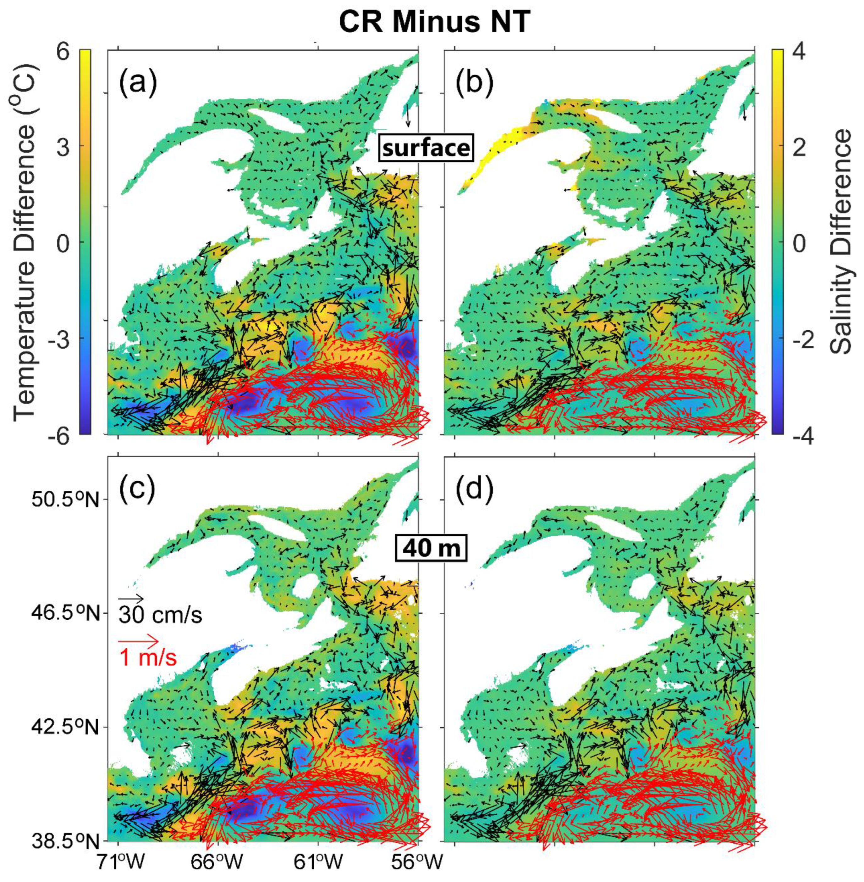
The role of tidal forcing on 3D circulation and hydrography over the GSL-ScS-GoM region and adjacent deep waters is examined based on the differences in model results between cases CR and NT. The tidal forcing is excluded in the latter case (
Table 1). In February 2018, the differences in the monthly-mean currents, temperature, and salinity at the sea surface (
,
) and at 40 m (
,
) between cases CR and NT have large values in the deep ocean region off the ScS-GoM, due to tide-induced modulations of the Gulf Stream, eddies, and meanders (
Figure 15). Tides also modify the intensities and locations of warm-core rings over the slope water region off the ScS-GoM, as shown by the large cyclonic and anticyclonic circulation differences
and
over the slope waters. As mentioned above, warm-core rings are associated with Gulf Stream instability processes related to the conversion between the potential energy and eddy kinetic energy. Tidal forcing affects these instability processes through tide-induced modulation of baroclinic dynamics.
Over the inner shelf of the ScS in February 2018, tides modify the southeastward outflow from the southeastern GSL and induce relatively large (between 0.1 m s
−1 and 0.2 m s
−1) and northeastward
and
(
Figure 15a,c). This indicates the important role of tide-induced horizontal advection over the ScS and southeastern GSL. Over coastal waters of the L2 domain, large values of
and in this month occur only over several local areas with strong tidal mixing (e.g., the BoF), intense tide-induced upwelling (e.g., coastal waters to the south of Cape Sable Island), and significantly stratified upper-column temperature or salinity (e.g., the SLE, with significant salinity vertical stratification). The relatively large and northeastward currents of
and
over the inner shelf of the ScS in this month result in northeastward transport of relatively warm and salty waters (associated with strong tidal mixing and tide-induced topographic upwelling; Kim and Smith, 1993) along the coast of south Nova Scotia.
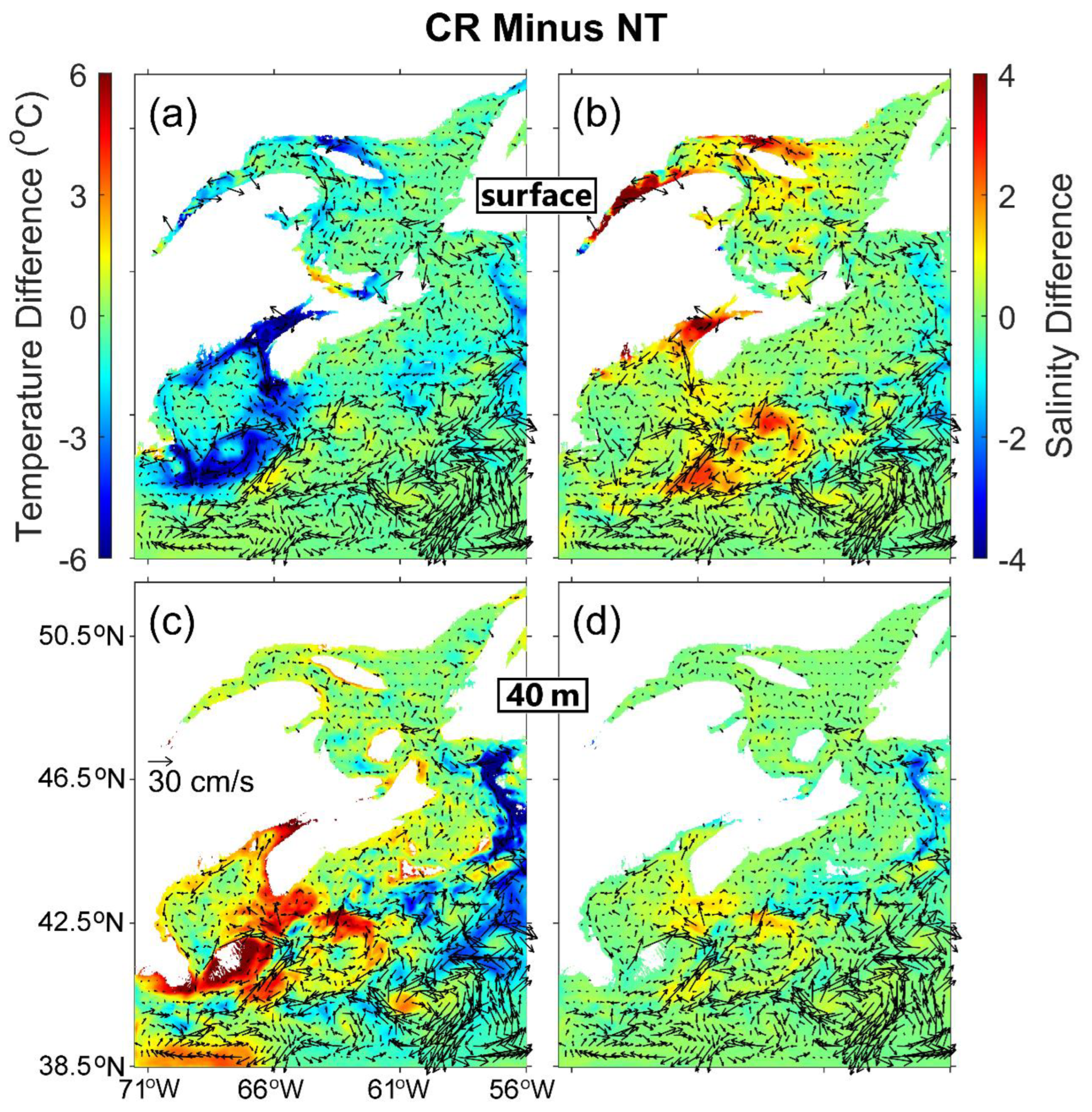
In August 2018, large values of
and
(
Figure 16a,c) occur in the BoF, northern GoM, southwestern ScS, western GSL, and Cabot Strait, which are mainly density-driven currents associated with tide-induced modulations of local density gradients. Some of these large
and
do not appear in February 2018 (e.g., in Cabot Strait and the northern GoM), mainly due to the strong convection and wind-induced mixing (resulting in typically small density gradients) in winter. The anticyclonic features of
and
around GeB (
Figure 16a,c) are associated with tidal rectification [
46]. The values of
and
around GeB are significantly larger in summer than in winter due to the reduced friction resulting from the weaker wind stress and stronger local density stratification in summer [
46].
In August 2018, the tidal forcing reduces the August-mean SST over the BoF, coastal waters of the northern GoM, GeB and adjacent waters, and swScS, with negative and large values of
up to −7 °C (
Figure 16a). Some noticeable SST cooling induced by tides also occurs in the northern GSL and the outer portion of the eastern ScS and adjacent waters. In summer, the large and positive net heat flux at the sea surface significantly warms the surface water and causes strong temperature vertical stratification in the top ~15 m over the L2 domain. Strong tide-induced vertical mixing and tidal rectification are the main reason for the significant SST cooling (subsurface warming) shown in
Figure 16a (
Figure 16c), with some contribution from the horizontal transport of different water masses by tide-induced mean currents. The tide-induced vertical mixing is also responsible for the large and positive values of
over the coastal and shelf waters of the L2 domain (up to ~4;
Figure 16b). In the deep waters off the ScS-GoM, there are small patches of positive and negative values of
due to tide-induced modulations of the Gulf Stream, Labrador Current (inshore branch in the southwestern NFS and offshore branch along the shelf break of the eastern ScS), eddies, meanders, and rings. These tide-induced modulations are also responsible for the large and positive
in the deep waters off the GoM and southwestern ScS, and for the large and negative values of
over the southeastern portion of the Laurentian Channel and deep waters off the southeastern ScS (
Figure 16c). In this month,
is relatively small in the GSL and northeastern ScS, but relatively large and positive over the swScS (
Figure 16d). The latter is associated with strong tidal mixing and tide-induced topographic upwelling [
47]. In the deep waters off the swScS and GoM, small patches of positive
occur mainly due to tide-induced modulations of fronts, eddies, and meanders.
To demonstrate the effect of tides on vertical stratification, we examine vertical profiles of monthly-mean temperature and salinity along the north-south transect EE’ off Yarmouth (
Figure 1c) based on model results produced by submodel L2 in cases CR (
,
) and NT (
,
). In both February and August 2018,
and
in case CR (
Figure 17a,c,e,g) are vertically uniform in the whole water columns over the northern section (within 50 km from the coast) and weakly stratified over the southern section of the transect (beyond 50 km from the coast). Without tides in case NT,
and
in February 2018 are nearly uniform in the surface mixed layer along transect EE’, mainly due to the strong winter convection caused by negative net heat flux and partially to the local wind-induced vertical mixing in the winter months (
Figure 17b,d). At depths below 30 m over the southern section of the transect,
and
in case NT are relatively warm and salty in February 2018, due to the effect of warm-core eddy separated from the Gulf Stream. A comparison of monthly-mean hydrographic profiles in February 2018 in cases CR and NT (
Figure 17a–d) indicates strong tide-induced vertical mixing at transect EE’, particularly over the northern section of the transect.
The August-mean
and
in 2018 in case CR (
Figure 17e,g) are vertically uniform in the whole water columns over the northern section, and weakly stratified over the southern section of transect EE’. Without tides in case NT, the August mean
and
are highly stratified in the top 20 m (
Figure 17f,h). The large differences in August-mean hydrography between cases CR and NT indicate the important role of strong tidal mixing in the vertical distributions of temperature and salinity over the inner and central shelves off Yarmouth. Over other areas with strong tides (e.g., the SLE and BoF), the vertical distributions of temperature and salinity are affected by tides in very similar ways.
To quantify the effects of tides on the monthly-mean currents over the swScS, we calculate the impact index (
) of tides at depth
based on the L3 model results using the method by Wang et al. [
9].
In February 2018, the values of
and
at 40 m (
Figure 18b) are highly comparable to their counterparts at the sea surface (
and
;
Figure 18a). In particular,
and
in this month are mostly northeastward or offshore in the middle shelf of swScS, except for a few narrow strips. This can be mainly explained by the tide-induced horizontal transport and the modulation effect of tides on the Nova Scotia Current, as well as other nonlinear circulation features. The February-mean tide-induced transport in 2018 (
Figure 15a,c) is generally northeastward over the swScS, weakening the alongshore (southwestward) transport of the Nova Scotia Current and thus enhancing its offshore transport (conservation of water mass). The values of
(
) are large in the middle shelf of the swScS, particularly over the areas with large
(
), quantifying the modulation effect of tides on the Nova Scotia Current and fine-scale gyres.
The August-mean
(
Figure 18c) in 2018 is large and westward to the south of Cape Sable Island, leading to a narrow strip of southwestward
over the inner shelf in this month, which enhance the inshore branch of the Nova Scotia Current at the sea surface. The August-mean
in 2018 also features a narrow strip of northeastward
in the middle shelf of the swScS, and a strong and cyclonic gyre of
over the southwestern portion of Emerald Basin (
Figure 1c), indicating the tide-induced modulation in the offshore branch of the Nova Scotia Current. In the rest of the swScS, the large values of
in this month are mainly associated with the tide-induced modulation of fine-scale gyres and meanders. In August 2018,
and
(
Figure 18d) at the sub-surface (40 m) show some general similarities with their counterparts at the sea surface (
Figure 18c) over most areas of the swScS, indicating that the tide-induced modulation in circulation occurs in the whole water column over the swScS.


