Article

Hydrodynamic and Particle Drift Modeling as a Support System for Maritime Search and Rescue (SAR) Emergencies: Application to the C-212 Aircraft Accident on 2 September, 2011, in the Juan Fernández Archipelago, Chile

1
Departamento de Obras Civiles, Universidad Técnica Federico Santa María, Valparaíso 2390123, Chile
2
Escuela de Ingeniería Civil Oceánica, Universidad de Valparaíso, Valparaíso 2362844, Chile
*
Author to whom correspondence should be addressed.
J. Mar. Sci. Eng. 2022, 10(11), 1649; https://doi.org/10.3390/jmse10111649
Submission received: 22 September 2022 / Revised: 24 October 2022 / Accepted: 25 October 2022 / Published: 3 November 2022
(This article belongs to the Section Marine Hazards)

Abstract

:
Search and rescue (SAR) refers to every operation aiming to find someone presumed lost, sick, or injured in remote or hard-to-access areas. This study presents the design of an operational system that supports maritime SAR emergencies by combining information from global hydrodynamic models (GHM) and a local hydrodynamic model (LHM) implemented in FVCOM. The output of these hydrodynamic models is used as input in a multiple particle drift estimator (MPDE) to estimate the trajectories of the floating elements derived from accidents in the ocean. The MPDE also includes trajectory estimates using the empirical LEEWAY formulation. The modeling system is validated with data collected during a SAR emergency that occurred on 2 September 2011, where a C-212 aircraft from the Chilean Air Force destined to the Juan Fernández Archipelago crashed in the ocean between the islands of Santa Clara and Robinson Crusoe. Trajectories were assessed in terms of the commonly used NCLS (normalized cumulative Lagrangian separation) performance indicator and a modified version, NCLS m o d , which considers both the movement and orientation of the trajectories. The LHM was executed in three scenarios: forced only with tide, forced with tide and wind combined, and forced only with wind. The performance of the different models varied in response to the ocean–atmosphere conditions and their local variations at the time of the accident. In times of calm wind, models with tidal influence performed better, while wind-forced models performed better when winds were greater than 7 km h 1 . The use of FVCOM (LHM) solved the coastal circulation and accounted for bathymetric effects in the Juan Fernández Archipelago area. This resulted in an improved variability and distribution of the modeled trajectories compared to the observed drifter trajectories. This work is the first study related to cases of maritime SAR emergencies in Chile, and provides a fast tool to estimate search areas based on an ensemble of particle drift and trajectory forecasts using multiple publicly available data sources.

1. Introduction

Search and rescue (SAR) refers to every operation aiming to find someone presumed lost, sick, or injured in remote or hard-access areas [1]. These operations include a wide range of events, which can be classified according to the zone of origin. The COSPAS-SARSAT [2] system classifies SAR emergencies as land, aviation, and maritime; the latter represented 40% of the total number of cases assessed by the COSPAS-SARSAT system in 2020. Regarding maritime accidents, the International Maritime Organization (IMO) has developed strategic plans for the prevention, survival, search, and rescue (International Aeronautical and Maritime Search and Rescue Manual, IAMSAR, 2019). IAMSAR [3] suggests that research and development associated with computerized tools, which make the search process more effective, needs to be promoted, and that numerical modeling output can be used as a valid source of information in the absence of field data.
At an international level, there are several studies on the use of hydrodynamic models in SAR emergency cases. Chen et al. [4] used FVCOM (Finite-Volume Community Ocean Model, e.g., Chen et al. [5]) combined with the WRF atmospheric model (Weather Research and Forecasting Model, e.g., Skamarock et al. [6]) to estimate the location of the Air France 447 accident that occurred in June 2009 in the Equatorial Atlantic Ocean with good results in terms of search area reduction. Cho et al. [7] developed and validated a maritime search and rescue operating system for the Yellow Sea and China’s east and south seas, combining the MOHID hydrodynamic model (e.g., [8]) and the WRF atmospheric model. Révelard et al. [9] recently proposed a methodology to measure the performance of Lagrangian particle drift simulations and their application in a real time data classification service as a built-in decision support system for SAR emergencies in the Iberian Peninsula (IBISAR, http://www.ibisar.es/es/, accessed on 15 September 2020). Other methods, such as the finite-scale Lyapunov exponent (FSLE) (e.g., [10,11,12,13]) have been used to define so-called Lagrangian coherent structures (LCSs) (e.g., [14]) and to map transport barriers and mixing regimes. LCSs have recently been used to optimize the search process by obtaining relevant information from the interpretation of OECSs (objective Eulerian coherent structures), and the estimation of regions with accumulation of floating objects [15].
A general characteristic of numerical tools designed to assist maritime SAR emergencies is their methodological diversification, which is associated with the region where the emergency occurs, data availability and the resources involved in the SAR response. The more developed systems use continuous monitoring systems via HF radars (e.g., IOOS, the Integrated Ocean Observing System of the United States, Muller-Karger et al. [16]), systems combining previously validated atmospheric and oceanic models which generate forecasts continuously (e.g., [17,18]), and signal satellite search systems (COPAS-SARSAT). The methods used to estimate trajectories show similar variability, varying between empirical methods, such as LEEWAY [19], which projects empirical relations between wind data at 10 m and the drift of known floating elements, deterministic methods (e.g., [20]), aiming to solve the physics of problem given certain initial conditions, and indirect methods such as TRAP estimation Serra et al. [15].
Given the diversification of systems and methods used in SAR support applications, their accuracy is highly dependent on data sources, calculation methods, and local environmental and forcing conditions. These support systems can show different levels of performance based on the performance measure (or index) used in their evaluation. All these variables affecting the accuracy and reliability of SAR support systems are difficult to evaluate under the same methodological standard. In an effort to combine sources and methods and assess them equally, the present work proposes a multiple particle drift estimator (MPDE) that considers the HYbrid Coordinate Ocean Model (HYCOM Chassignet et al. [21]) and the European Union’s MULTIOBS015004 [22] as global hydrodynamic models, ERA5 [23] as the global atmospheric model (GAM) and FVCOM [4] as a local hydrodynamic model (MHL). The MPDE uses these data sources and considers a direct calculation of trajectories (velocity taken directly from the model source), deterministic (velocity obtained from a drag force balance, e.g., Di Maio et al. [20]) and through the LEEWAY empirical model [19]. Modeled trajectories were contrasted with field data from surface drifters and accident findings obtained during a SAR emergency that occurred in the Juan Fernández Archipelago, Chile, on 2 September 2011. In this accident, a C-212 aircraft from the Chilean Air Force (FACh) crashed in the sea between the island of Santa Clara and Robinson Crusoe. This work is the first study related to cases of maritime SAR emergencies in Chile and aims to develop a practical modeling approach that provides fast and optimized estimates of search areas based on an ensemble of particle drift and trajectory forecasts that uses multiple data sources. The paper is organized as follows: Section 2.1 details the area of study, the SAR emergency and the measurements used as case study; Section 2 presents the methodology, including details of the hydrodynamic models, trajectory calculation methods and the performance analysis measures; Section 3 presents the results, with a focus on the performance analysis between the observed and modeled trajectories; finally, Section 4 discusses the main results and presents the conclusions.

2. Materials and Methods

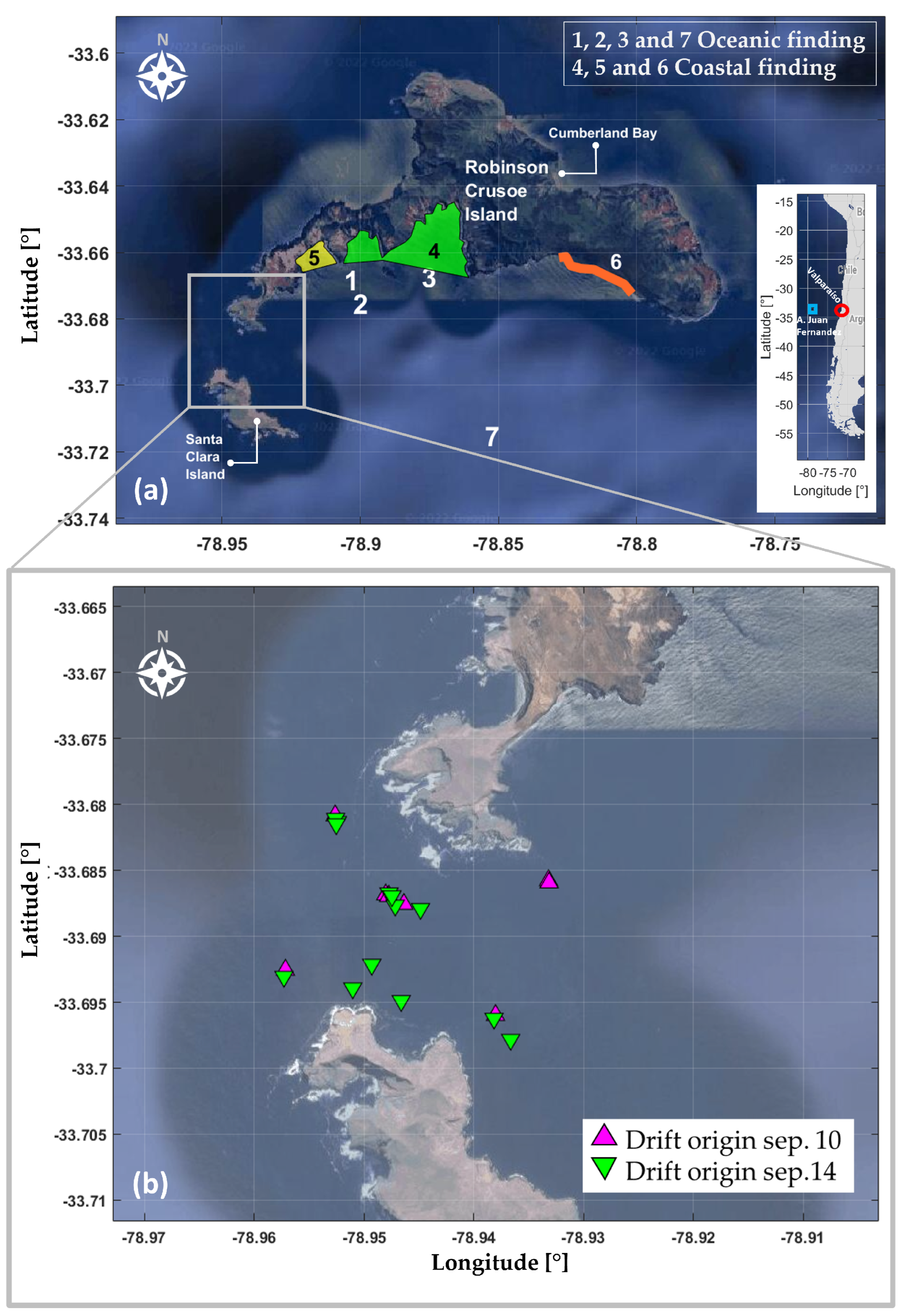
2.1. Study Area and SAR Emergency

The study area was the coastal ocean off the Robinson Crusoe and Santa Clara islands, which are part of the Juan Fernández Archipelago and are located approximately 670 km from the coast of Valparaíso, in central Chile (Figure 1). These islands are of volcanic origin, mountainous (maximum elevation of 915 m, Yunque hill), and steep [24]. According to available data in the area, the strength of tidal currents frequently interrupts fishing activities [24]. Current measurements conducted in the area between the Santa Clara and Robinson Crusoe Islands indicate that under calm wind conditions (wind speed < 7 km/h) the surface currents are directed towards the southeast during flood tide and towards the northwest during ebb tides [24]. In the presence of greater magnitude (>7 km/h) and persistent winds from the northwest, the surface currents show a predominantly southeast direction [24].
The light transport aircraft Casa-212 Aviocar of the Chilean Air Force (FACh) took off at 14:00 HL (17:00 UTC) from Arturo Merino Benítez Airport in Santiago, Chile, on 2 September 2011, destined to Robinson Crusoe’s airdrome (Figure 1a). The plane transported 21 people between passengers and crew. Near the island and after several failed landing attempts, contact with the aircraft was lost at 17:48 HL (20:48 UTC). Gracia [25] reported that adverse conditions resulting from high wind shear and the complex orography of the area caused atmospheric instabilities with strong turbulence and vertical flows, which resulted in a limited ability to control the aircraft at an altitude of ∼200 m. During the SAR emergency, the Hydrography and Ocean Service from the Chilean Navy (SHOA) conducted measurements using surface and subsurface drifters (1.5, 10, and 20 m deep) on 10 and 14 September 2011 (Figure 1b). Both the Chilean Navy and the National Air Force (FACh) oversaw the collection of remains at the time of the accident, which in general corresponded to heterogeneous remains characteristic of a high-impact accident and were mainly found in the southern area of the bay of Robinson Crusoe (Figure 1a).

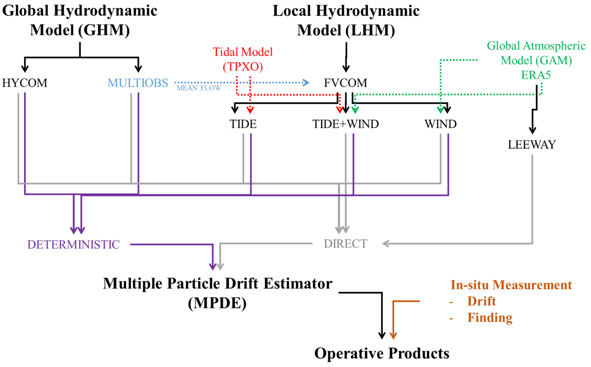
2.2. Model Components and Data Sources

The selection of global hydrodynamic model (GHM) and global atmospheric model (GAM) was based on data availability at the time of the accident. Selection of the local hydrodynamic model (LHM) was based on open-source code and their capacity to adapt to coastal areas using unstructured grids. The flowchart of the proposed modeling scheme is detailed in Figure 2, and the components are described in the following subsections.

2.2.1. Global Hydrodynamic and Atmospheric Models (GHM and GAM)

We used reanalysis data of the GOFS 3.1 model (identified as HYCOM) from the Center for Ocean-Atmospheric Prediction Studies (COAPS) in the United States (https://www.hycom.org/dataserver/gofs-3pt1/analysis, accessed on 15 September 2020). This model couples the global HYCOM Model (HYbrid Coordinate Ocean Model, e.g., Chassignet et al. [21]) and the CICE model (Los Álamos Sea Ice Model, e.g., Hunke and Lipscomb [26]). The spatial and temporal resolutions of the HYCOM model are 0.08° (1/12°) and 3 h, respectively. Additionally, we used reanalysis data from the MULTIOBS015004 model (hereafter MULTIOBS, e.g., Rio et al. [22]) generated by the CLS Production Center (MULTIOBS-CLS-TOULOUSE-FR) and downloaded from the Earth Observation Programme COPERNICUS from the European Union (https://resources.marine.copernicus.eu/product-detail/MULTIOBS_GLO_PHY_REP_015_004/INFORMATION, accessed on 16 September 2020). The spatial and temporal resolutions of the MULTIOBS model are 0.25° and 3 h, respectively. The atmospheric component was taken from the global atmospheric model (GAM) ERA5 [23] (https://cds.climate.copernicus.eu/cdsapp#!/dataset/reanalysis-era5-single-levels, accessed on 16 September 2020), and corresponded to wind data at an elevation of 10 m. This model was used for forcing the local hydrodynamic model (LHM), to compute trajectories through the LEEWAY empirical formula and as the atmospheric component for solving the deterministic drag force balance (see Section 2.2.3). This product is generated by the Integrated Forecast System (IFS) of the European Centre for Medium-Range Weather Forecasts (ECMWF). The spatial and temporal resolutions of ERA5 data are 0.25 ° ) and 3 h, respectively.

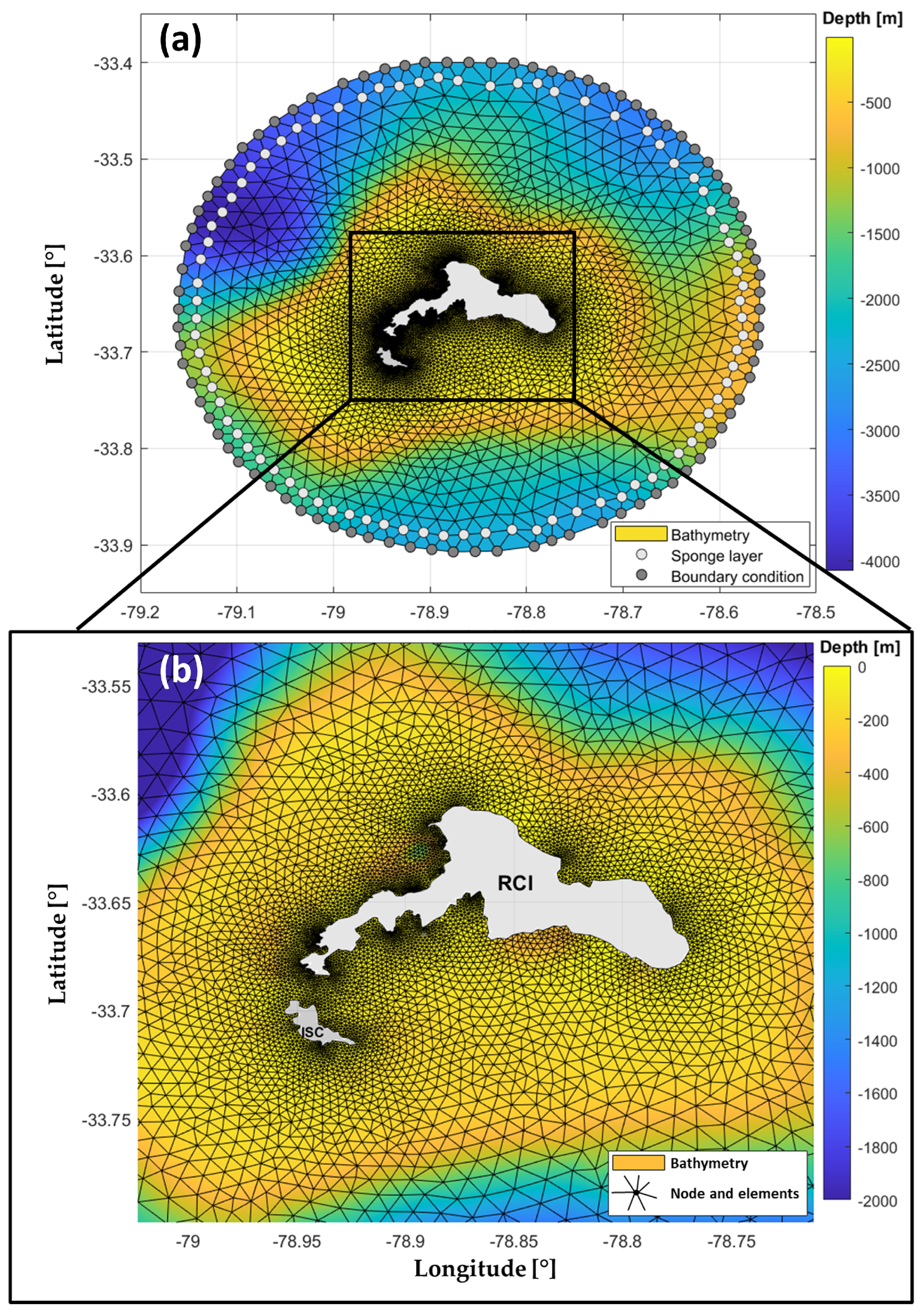
2.2.2. Local Hydrodynamic Model (LHM)

The LHM was implemented in FVCOM (Finite-Volume Community Ocean Model). The model was originally developed by Chen et al. [5] and solves the primitive governing Equations (3D) in integral form using Cartesian or spherical coordinates through flux calculations between triangular control volume elements. The FVCOM model has been used in multiple studies of coastal circulation, demonstrating its capacity to solve dynamics associated with wind, tide, and waves (e.g., [27,28,29,30]). For details about the model, governing equations, and parameterizations, refer to Chen et al. [5].
FVCOM was set up to obtain data from up to 10 days before the moment of the accident, which is the period used for model stabilization. The temporal resolution of the internal calculations is 1 s, while the output was saved every 30 min. Model bathymetry was obtained from single-beam and multi-beam measurements conducted by SHOA in coastal areas, and from GEBCO 2019 data [31] in deep ocean areas. In areas of scarce bathymetric data, depth was extracted from the nearest bathymetric data. The bathymetry was smoothed through linear interpolation of triangular elements. Using the algorithms described by Engwirda [32], we generated an unstructured grid of 6336 nodes and 12,073 vertexes with a maximum spacing of ∼2.6 km offshore and a minimum of ∼46 m at the coast (Figure 3). Once the grid was created, we selected the nodes for the integration of boundary conditions and specified sponge nodes (Figure 3), which are necessary to prevent energy accumulation and inward energy propagation from the boundaries [33].
Temperature and salinity boundary conditions were taken from historical profiles collected in the area [34]. We considered the temperature and salinity fields varying between 15 °C and 2 °C and between 33.8 psu and 34.6 psu from the surface to the bottom, respectively. These profiles were kept constant during the modeling to isolate the effect of forcings with higher variability in short timescales (hours to days) such as tides and wind. Currents were incorporated into the model in terms of an average discharge (m 3 s 1 ) calculated from the east and west flow components (u and v, respectively) of the MULTIOBS model, considering the volume of the triangular element at each vertical layer. The depth-averaged flow was incorporated at the boundary nodes (Figure 3).
The LHM scenarios were specified based on atmospheric and oceanic area records, which describe a complex interaction between wind effects and tidal currents in the channel between island of Santa Clara and Robinson Crusoe [24]. Thus, the implementation of FVCOM was separated into the following scenarios: only tide (T), only wind (W), and tide and wind (T + W). For the tidal forcing, we used the amplitude and phase obtained from the TPXO global model [35] and prescribed the M2, S2, N2, K2, and K1 harmonic constituents, which correspond to the mixed tide regime that is typical of the Chilean coast [36]. The tidal forcing was prescribed at the boundary nodes (Figure 3). The wind forcing was incorporated from the ERA5 model data in every surface node in the grid. Figure 4 shows the comparison between the TPXO data and tidal data from Cumberland Bay (see Figure 1a for the location of this station), as well as a comparison between ERA5 wind data and wind records from the General Directorate of Civil Aviation (DGAC) weather station from Bahia Cumberland during the time of the accident. Good agreement is observed between the tidal level in the TPXO model and the tide measured in Cumberland Bay, with a correlation of R = 0.94 (p-value < 0.05). Similarly, we observed good agreement between the measured wind and the wind data extracted from ERA5; however, the meridional component (V) showed a much better correlation ( R = 0.96 ) than the zonal component (U, R = 0.37 ).
We selected a semi-implicit numerical scheme to solve for the non-hydrostatic pressure [37]. The turbulence closure model was the q q l Mellor–Yamada level 2.5 [38], where q is the turbulence kinetic energy and l is the turbulence macroscale. The horizontal and vertical mixing coefficients were 0.4 and 1.0 × 10 6 m 2 s 1 , respectively, (e.g., [33]). The bottom drag coefficient C d b was calculated using the logarithmic law of the wall [39] (Equation (1)) and imposing a no-slip condition at the bottom boundary. C d b was computed using a bottom roughness length scale of z 0 = 0.001 and defining a minimum value of C d b = 0.0025 :
C d b = m a x [ k 2 / l n ( z a b / z 0 ) 2 , 0.0025 ]
where k = 0.4 corresponds to the Von Kárman constant, and z a b corresponds to height above the bottom.

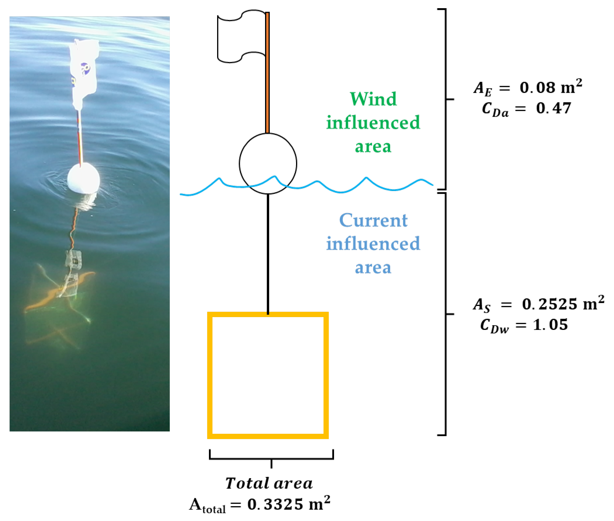
2.2.3. Multiple Particle Drift Estimator (MPDE)

We implemented a multiple particle drift estimator (EMDP) to determine the trajectories of floating elements during the SAR emergency which uses several information sources and various methodologies to estimate drift velocities of particles and their trajectories at the surface. The reason for implementing an EMDP is that during a maritime SAR emergency, a scenario with multiple solutions combined with the existence of in situ data facilitate the estimation, almost in real time, of particle trajectories and evaluate their performance. Consequently, the MPDE can guide and assist authorities overseeing the emergency. The EMDP is based on the resolution of the ordinary differential Equation (e.g., [40]):
d x d t = v o b x ( t ) , t
where x ( t ) corresponds to the initial position of the object (or particle), and v o b corresponds to the velocity vector. v o b was determined by two methods: (i) a direct method (hereafter, Dir.), where the velocity was set to be equal to the surface velocity fields obtained from the GHM and LHM, and (ii) a deterministic method (hereafter, Det.) based on the methodology developed by Di Maio et al. [20], where v o b was estimated from a stationary drag force balance of a partially submerged symmetric object, neglecting the effect of lift [20]:
F W + F E + F D l + F D a = 0
where F W is the weight of the object, F B is the buoyancy force, F D l is the drag force exerted by the fluid on the object, and F D a is the drag force exerted by air on the object. In the vertical axis, we assumed that F W + F B = 0 , that is, that the object had neutral buoyancy. The problem is further simplified by assuming that the emerged and submerged proportion of the object was known and invariant ( R E and R S , respectively). In the horizontal axis, the forces F D l and F D a are responsible for the surface transport of the object. The drag force F D experienced by a sphere of radius R and velocity V is taken from Stokes’ law for viscous fluids with dynamic viscosity μ , F D = 6 π μ R V (e.g., [41]). Introducing F D into Equation (3) (in the horizontal plane) and considering the velocity v o b as the velocity relative to the object, we get
μ l R S v c v o b + μ a R E v a v o b = 0
where v c and v a are the velocity of surface currents and wind, respectively. In Equation (4), μ l corresponds to the dynamic viscosity of water and μ a corresponds to the dynamic viscosity of air. Considering the dimensionless explicit formulation of the drag coefficient C D for a body submerged in terms of the Reynolds number ( R e ) and neglecting the effects of compressibility (e.g., [41]), Equation (4) can be rewritten as follows:
1 2 C D w ρ w A S v c v o b 2 + 1 2 C D a ρ a A E v a v o b 2 = 0
where C D w is the drag coefficient under water, ρ w is the density of seawater, A S is the submerged area of the object, C D a is the drag coefficient for the emerged part of the object, ρ a is the density of air, and A E is the emerged area of the object. Equation (5) was solved numerically for the variable v o b .
In parallel, we implemented the LEEWAY method based on the work of Hufford and Broida [19] and developed extensively in the LEEWAY divergence reports of the U.S. Coast Guard Research and Development Center (e.g., [42]). This method considers wind data 10 m above the surface, which we extracted from the GAM ERA5. We estimated the downwind component (downwind, DWL) and its crosswind component (crosswind, CWL) from wind data at 10 m according to (e.g., [42]):
D W L ( cm   s 1 ) = m D W L ( % ) W 10 ( m   s 1 ) + b d ( cm   s 1 )
C W L ( cm   s 1 ) = m C W L ( % ) W 10 ( m   s 1 ) + b d ( cm   s 1 )
where m D W L and m C W L are the regression slopes for the DWL and CWL coefficients, respectively, and b d is the intercept of the regression [42]. We considered the optimal regression values determined empirically and tabulated by Allen [42] for different categories of drift elements. The CWL component acts in positive and negative directions and operates under a random function with a standard error, which is also tabulated in Allen [42], resolving for the horizontal divergence. However, in this work, the divergence parameter was incorporated equally to all models, scenarios, and methods studied; therefore, the trajectories obtained through LEEWAY considered only the DWL parameter (Equation (6)).
The velocity of the object v o b was obtained using a fourth-order and four-stage Runge–Kutta explicit scheme [40,43], which is the same method used by FVCOM to solve trajectories internally [33]. Here, the algorithm was solved externally and in 2D, transforming the latitude and longitude coordinates to UTM north and east coordinates, respectively, and assuming a constant and continuous (but variable in space) surface velocity vector for each time interval. We note that the time step Δ t used in trajectory calculations corresponds to the temporal resolution of each of the models used. To secure numerical stability and compensate for the low temporal resolution of GHM compared to the duration of the in situ measurements, the time step was increased by six times in the GHM (linear interpolation) to have the same temporal resolution of the LHM outputs.
Finally, to capture the natural dispersion of the meso- and submesoscale currents, we imposed a normally distributed directional divergence perturbation at each time step [44]. This directional divergence was less than 20° in all cases and corresponds to maximum values typical of LEEWAY divergence angles, as estimated by Allen and Plourde [44] for several categories of floating elements. Moreover, these values are associated with the coastal directional dispersion values reported by Ohlmann et al. [45] with respect to submesoscale processes using Lagrangian drifters and tracers, where average rotation values of ∼18 ° were measured in 2.5 h trajectory. This normally distributed directional divergence step was used in all estimated trajectories, regardless of the method used for their computation.

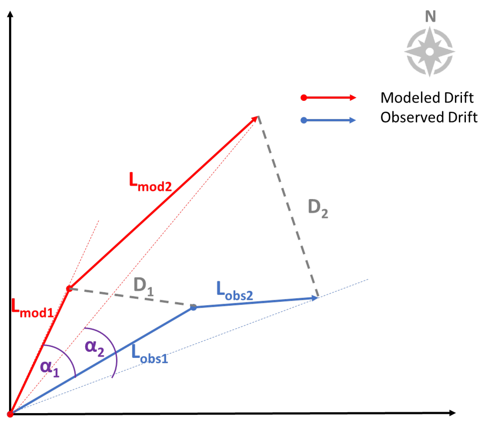
2.2.4. Performance Analysis

We conducted a quantitative performance analysis of modeled trajectories by comparison to in situ drift trajectory measurements performed by SHOA on 10 and 14 September, during the SAR emergency. In this measurement campaign, surface drifters (Figure 5) were released at different locations between Santa Clara Island and Robinson Crusoe Island (Figure 1b).
Considering the dimensions of the drifters used at the time of the accident (Figure 5), we estimated that A E = 0.08 m 2 and A S = 0.25 m 2 , and we used those values in the deterministic analysis of particle drift trajectories (drag force balance). We used the drag coefficients proposed by [46] for objects interacting with turbulent flows ( R e 10 4 10 6 ). Because of the shape of the drifter, the drag coefficient was C D a = 0.47 for the emerged portion, which corresponds to a sphere [46], whereas a C D w = 1.05 was used for the submerged part, corresponding to a square shape [46]. We note that the Reynolds number R e used in Di Maio et al. [20] varied between 1.65 × 10 5 and 1.68 × 10 5 . Finally, for the LEEWAY analysis, we used the values tabulated in Allen [42] for a person floating in the surface (PIW, person in water) in a sitting position (given the similarity with the geometry of the buoy), for which m D W L = 1.06 % and b d = 8.3 cm s 1 .
The quantitative performance of the modeled trajectories was assessed using a modified version of the NCLS (normalized cumulative Lagrangian separation) index, which in its original version is [9,47]:
N C L S = i = 1 N D i i = 1 N L o b s , i
where N is the number of observations, D i is the difference between modeled and observed distances, and L o b s , i is the path of the observed drifter. The modified NCLS version (NCLS m o d ) includes an angular proportion α i α r e f to quantify the performance with respect to the orientation of the trajectories (Figure 6), and is given by
N C L S m o d = i = 1 N α i α r e f + D i i = 1 N L o b s , i
where α i is the angle formed between L o b s , i , L m o d , i , and the origin and α r e f is an angular calibration parameter that adjusts for the orders of magnitude between distances and angles. In the present work, the angular proportion α i α r e f was adjusted with α r e f = 1 ° , considering the spatial scale of the study. This performance index, termed NCLS m o d , is not only conditioned by the path of trajectories but also by their orientation, which is particularly relevant in trajectories where there is a change in orientation. The mathematical evaluation and comparison of the NCLS and NCLS m o d indices is shown in Appendix A for idealized test trajectories.
Modeled trajectories were also evaluated qualitatively by verifying arrivals into regions where accident remains were found during the SAR emergency (Figure 1, colored areas). A total of 260 particles were released in a 300 m radius around the point of the accident every 30 min and over 6 h from the time of the accident, and their movement was assessed throughout the next 6 days. Similarly to the quantitative assessment, we used a normally distributed directional divergence perturbation not greater than 20 ° at each time step (e.g., [44,45]). For the estimation of trajectories using the deterministic model, we assumed a cylinder with A E = A S = 0.5 m 2 and C D a = C D w = 0.82 [46]. In trajectory calculations using the LEEWAY method, we again assumed the regression parameters of Allen [42] for a PIW in a sitting position. The success of the trajectories was evaluated based on the arrival of particles to the polygons highlighted in Figure 1a.

3. Results

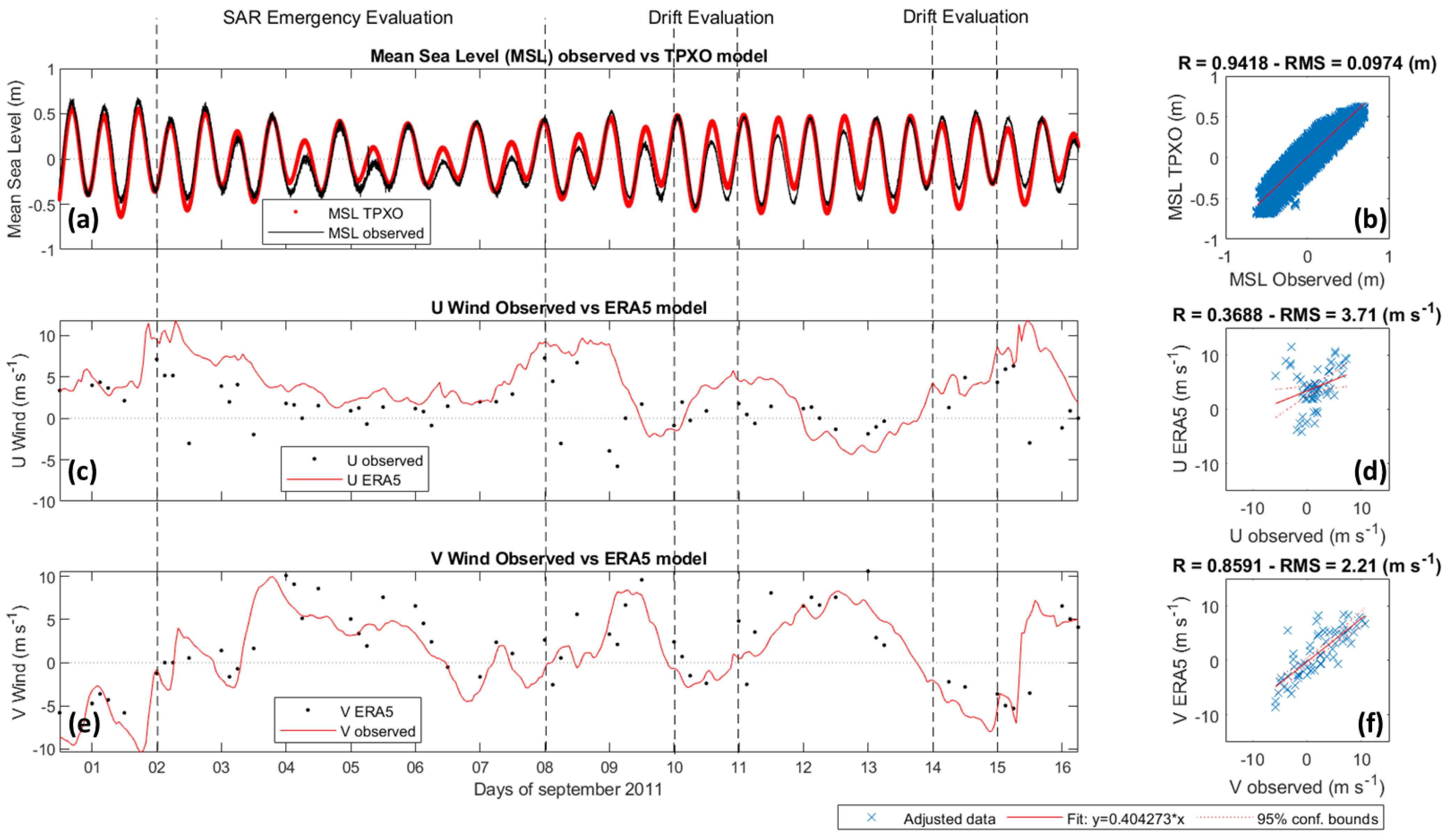
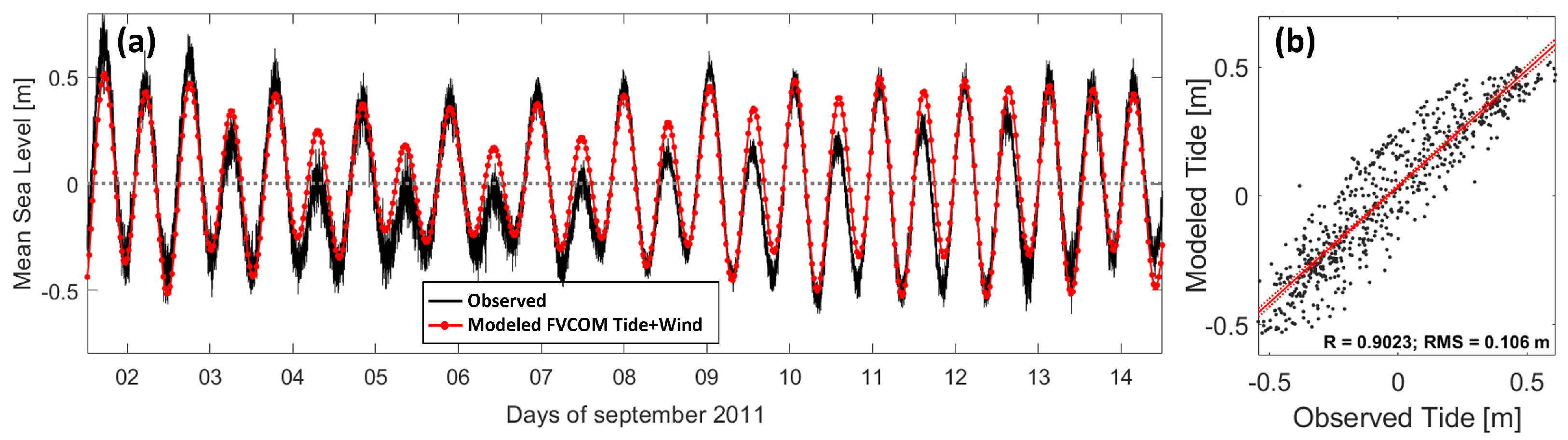
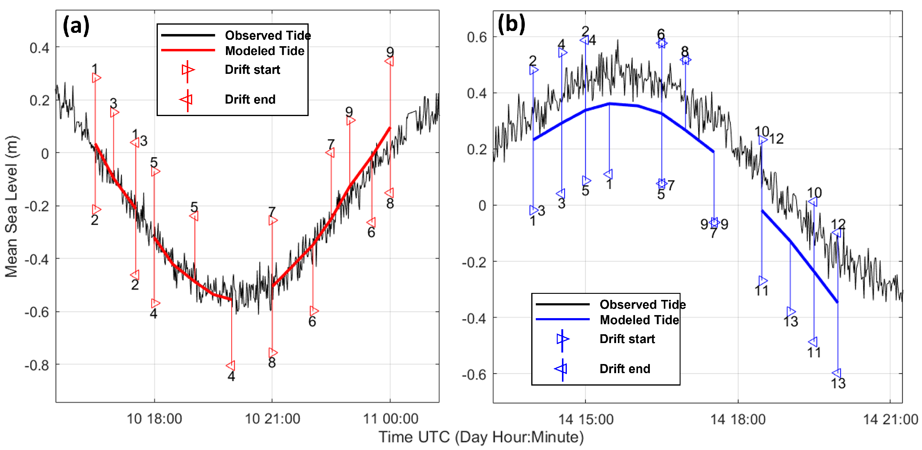
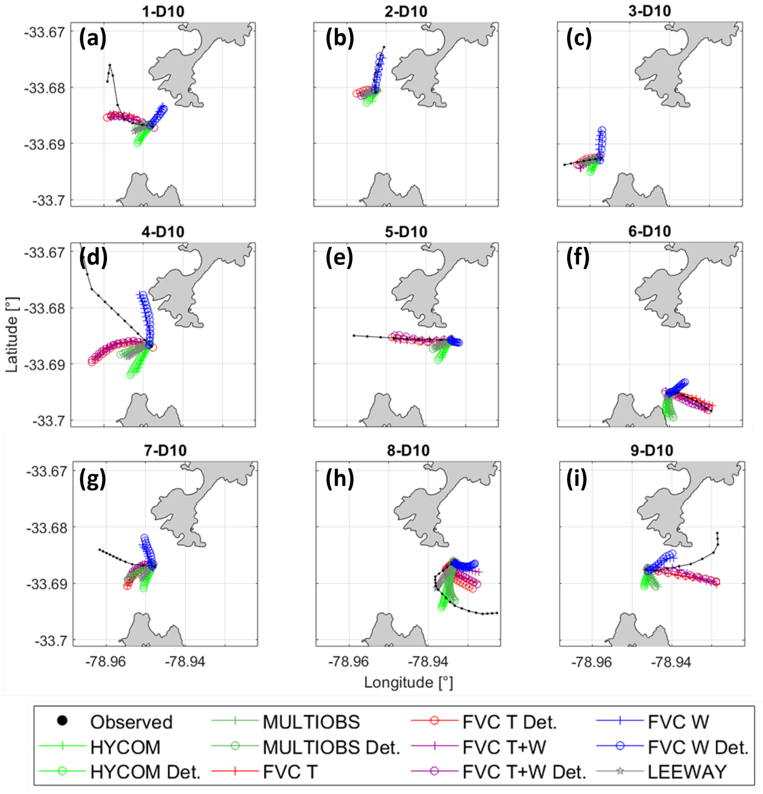
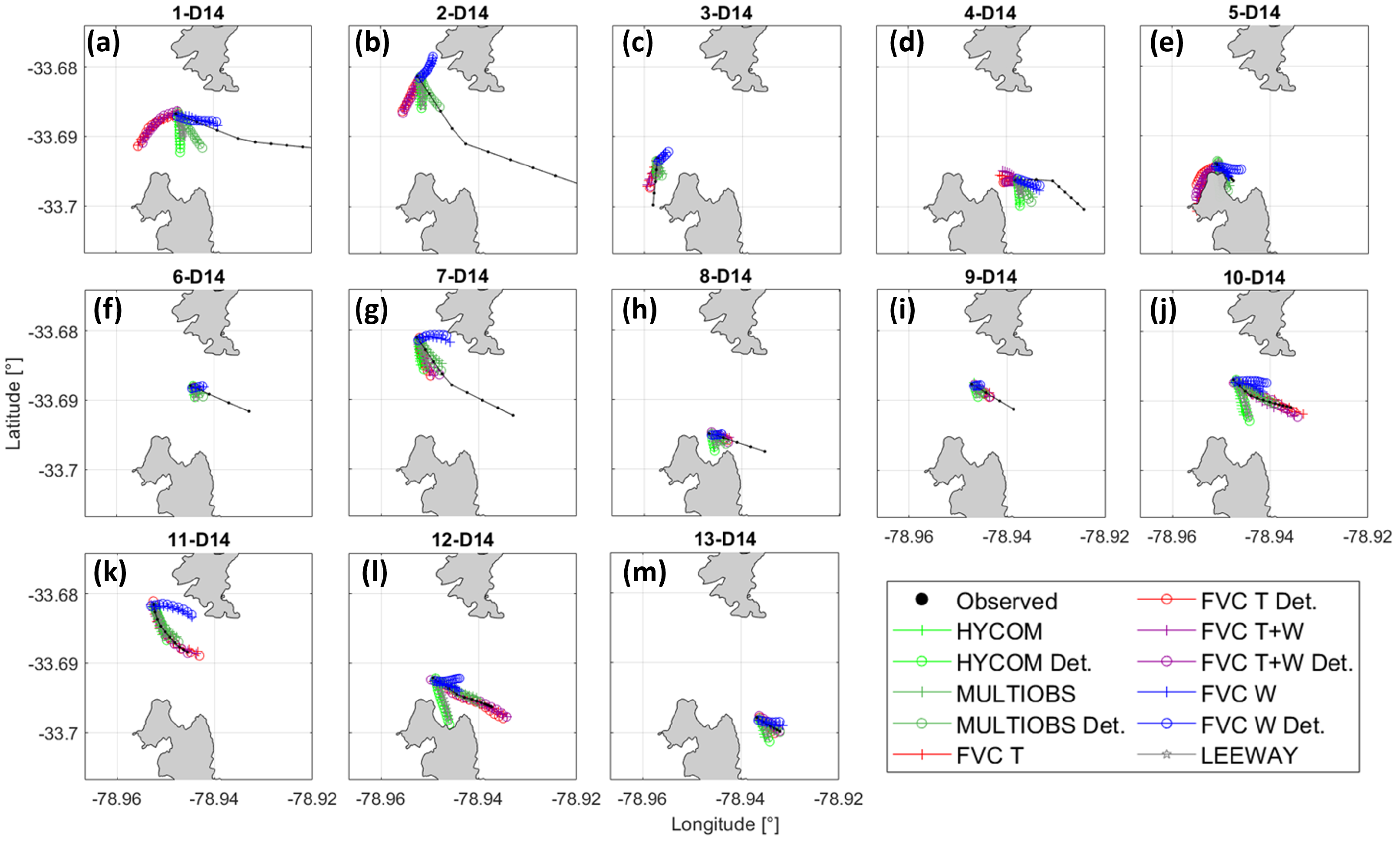
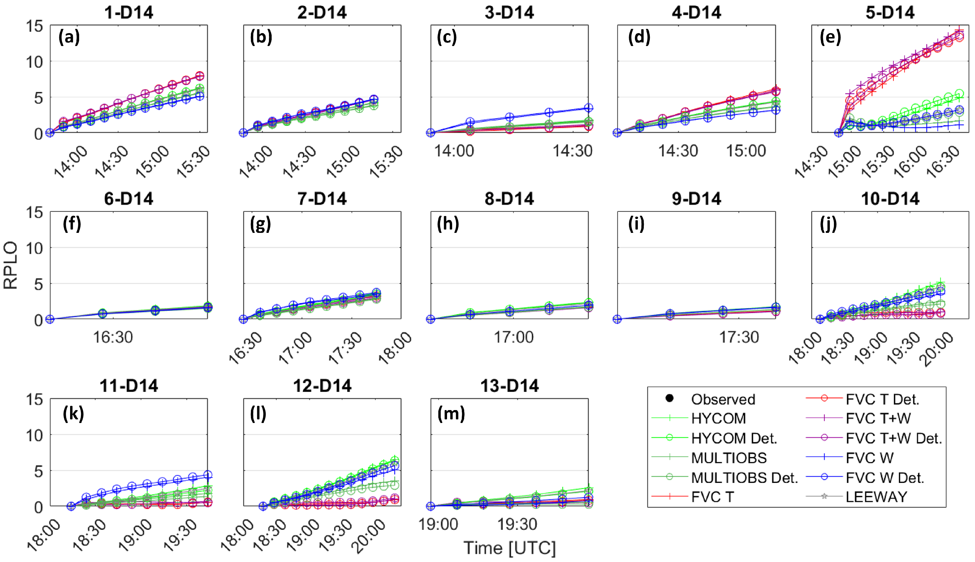
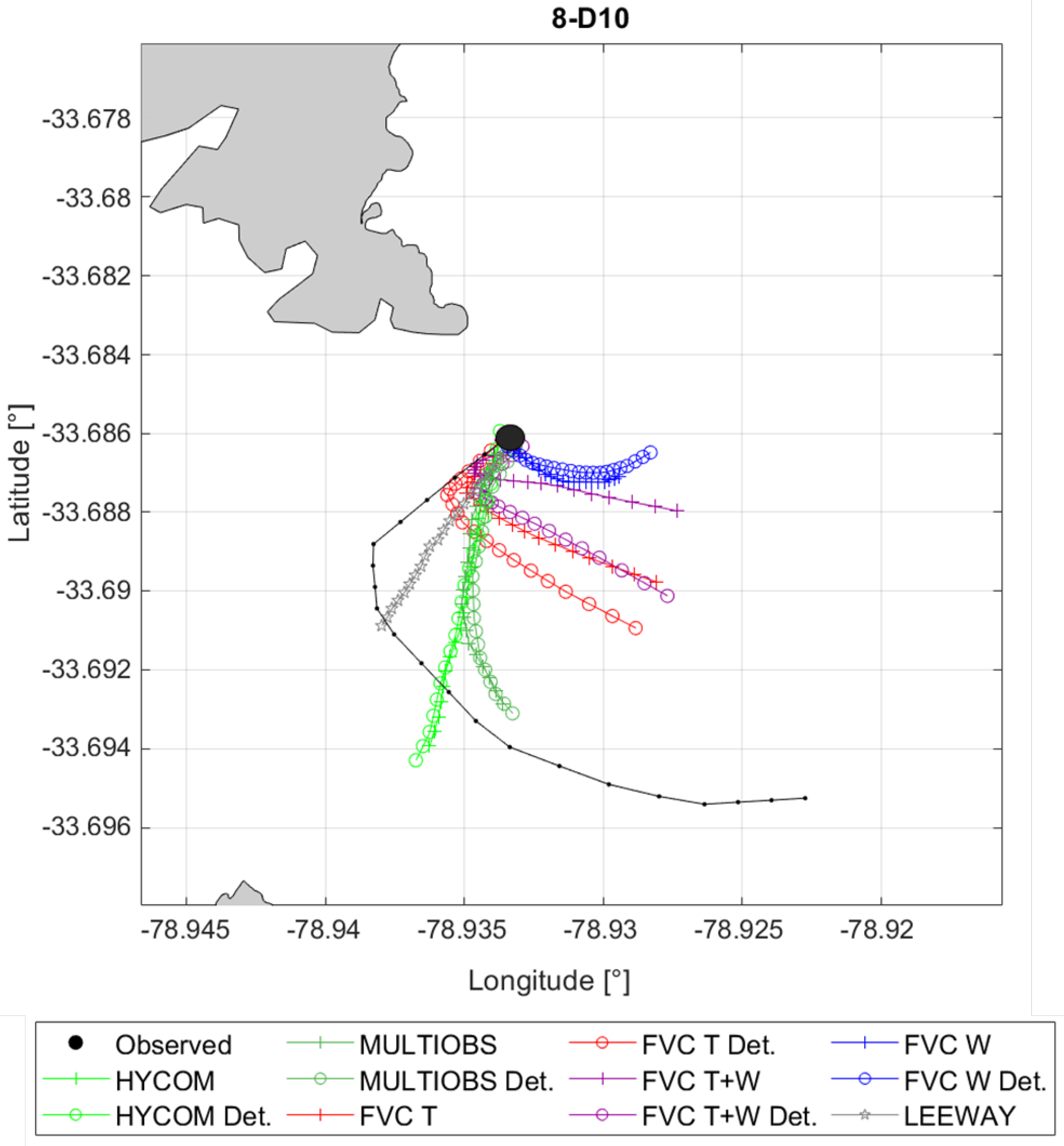
3.1. Model Validation and Trajectory Calibrations

Considering the time frame of the FVCOM hydrodynamic modeling and its short duration, model validation could only be done in terms of comparing modeled water surface elevation with in situ tidal data from the SHOA sea level station located in Cumberland Bay. Figure 7 shows the measured tidal elevation and model results from the FVCOM Tide + Wind case, which demonstrate good agreement between the modeled and measured data. We note that the surface elevation results are very similar for the FVCOM Tide scenario (not shown); however, the surface current fields generated by these scenarios are different, which is reflected in marked differences in modeled trajectories. We observe that model performance is better during spring tides than during neap tides; in the latter, the models underestimated the daytime tide level variation and resulted in an overestimation of the lowest high tide of the day (Figure 7a,b). This overestimation may stem from the use of TPXO tidal forcing in the LHM (Figure 4).
Prior to the quantitative performance analysis using NCLS and NCLS m o d , we calibrated modeled trajectories obtained from FVCOM considering that high-resolution models commonly create more energetic dynamics than those observed (e.g., [9]). For this, we analyzed the modeled trajectories and normalized them by a factor obtained by comparison to observed trajectories (Figure 8). Figure 8 shows that the FVCOM scenarios forced with Tide and Tide + Wind overestimate trajectories by approximately 60% (on average) when compared to measured trajectories, while the FVCOM Wind scenario underestimates trajectories (on average) by 70%. Calibration was executed by scaling the resulting velocities from the LHM by the trajectory underestimation and overestimation percentages. These calibrated velocities are re-entered into the EMDP for trajectory computations. LHMs frequently contain small-scale effects that are not present in reality or that occur displaced in space or time (e.g., [9,48,49,50]). Consequently, the start of modeled trajectories was specified considering a spatio-temporal lag of ±1 h in a 100 m radius centered on the point of origin of the drifter deployments.

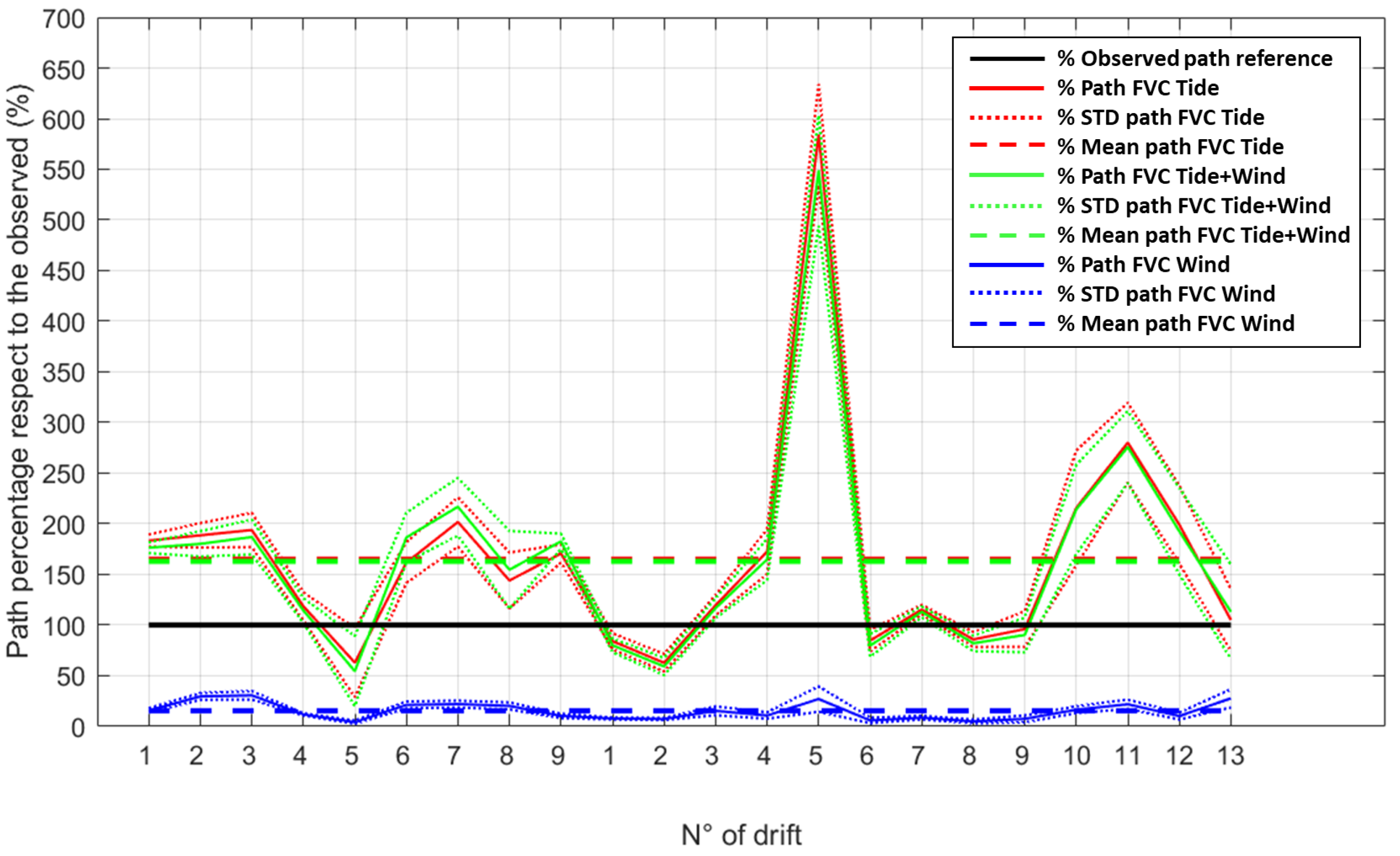
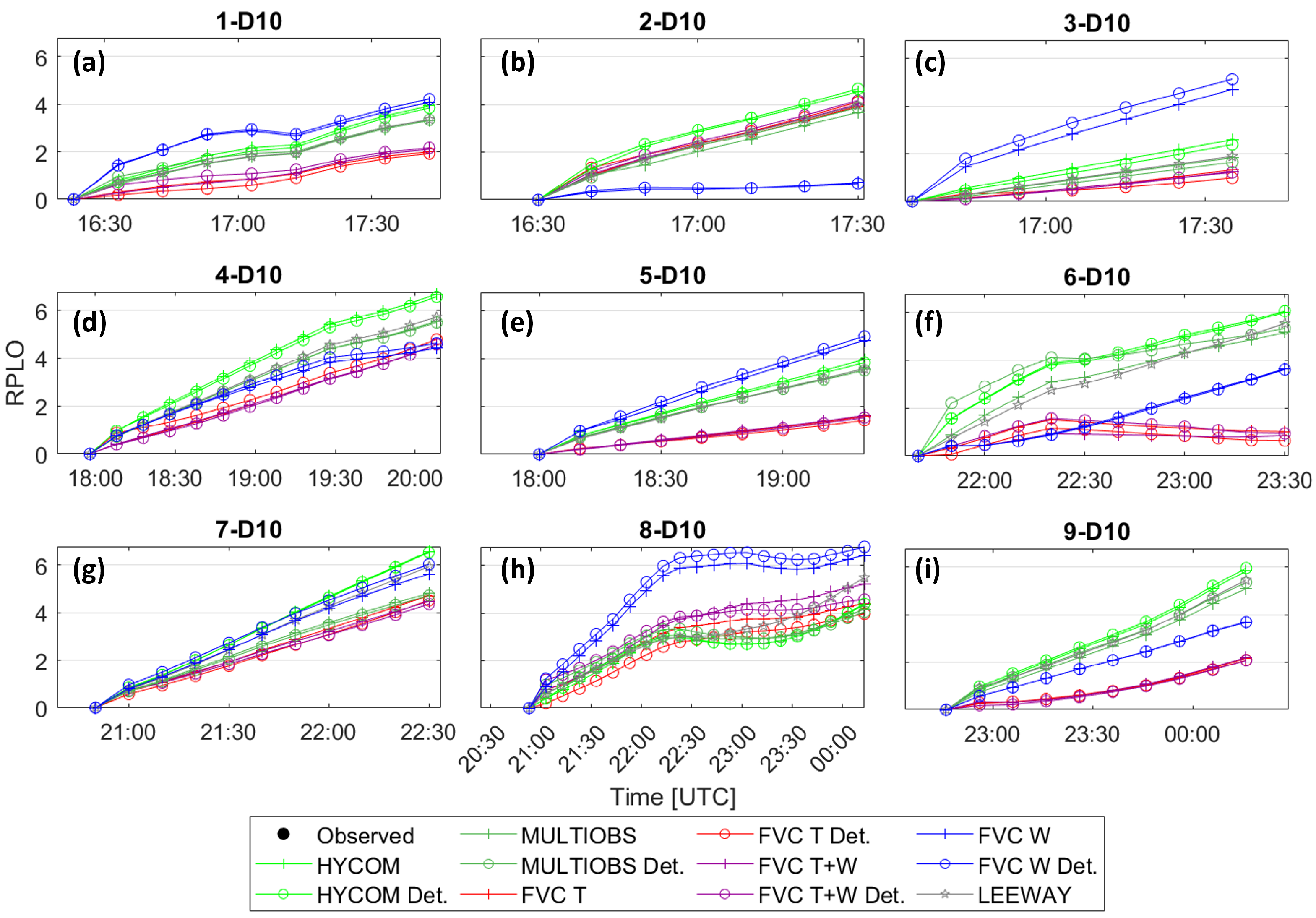
3.2. Quantitative Performance Analysis

Figure 9 shows the observed and modeled tidal elevation (FVCOM), along with the measurement period for each drifter release. Figure 10 and Figure 11 show the trajectories with best NCLS m o d for 10 and 14 September, respectively. For 10 September, we observe a change in direction of the measured trajectories that was associated with the change in tidal phase at approximately 20:00 UTC (Figure 10). We observe that only the models FVCOM Tide and FVCOM Tide + Wind achieve the reproduction of the tidal phase change (between ebb and flood) occurring that day. FVCOM Wind registered a direction variation going from north to the northeast, while the GHMs showed a change in direction from the southwest to the south. For 14 September (Figure 12), observed trajectories showed movement towards the SE, which is equivalent to flood tide conditions although most of the measurements were conducted during ebb tide (Figure 9b). This suggests that during that day there were winds of greater intensity blowing to the SE, which caused a generalized transport towards the east. The scenarios FVCOM Tide and Tide + Wind showed good agreement with the tidal phase, exhibiting trajectories corresponding to a southeast flow for drifters released during flood tide (1 to 5). FVCOM Wind showed better results, but trajectories deviated towards the north. The GHMs were almost invariant, with a preference for the south–southeast direction, resulting in a good performance for most of the compared drifts (Figure 11).
Figure 12 and Figure 13 show the temporal evolution of NCLS m o d values for the trajectories with the best performance for 10 and 14 September, respectively. The daily median NCLS m o d value for each model is shown in Table A1 and Table A2. For comparison, Table A1 and Table A2 also show the value of the standard NCLS index. For 10 September (Figure 12), we observe that NCLS m o d values lower than two align with the trajectories with the best performance shown in Figure 11. The LHMs outperformed the GHMs in the nine cases, five of which are represented by FVCOM Tide Det. (NCLS m o d of 1.93, 0.99, 1.43, 0.64, and 3.97 for the 1D10, 3D10, 5D10, 6D10, and 8D10 drifters, respectively), two are represented by FVCOM Tide + Wind Det. (NCLS m o d of 4.35 and 2.07 for the 7D10 and 9D10 drifters, respectively), one is represented by FVCOM Wind (NCLS m o d of 0.67 for 2D10), and one is represented by FVCOM Wind Det. (NCLS m o d of 4.42 for 4D10). The daily mean NCLS m o d values showed the best performance for the trajectories generated by FVCOM Tide Det. (2.71), with a final angular deviation of 32.5 ° , a mean angular deviation of 23.1 ° , and a standard deviation of ±8.9 ° . This scenario also registered the lowest difference between modeled and observed trajectories (562.4 m). The global analysis of the total number of trajectories generated using the spatio-temporal lag also showed the best performance associated with the FVCOM Tide Det. case, with a mean NCLS m o d value of 5.22, a final angular deviation of 71.6°, a mean angular deviation of 68.9°, and a standard deviation of ±34.6°, and path difference of 639.6 m.
For 14 September (Figure 13), we observe that NCLS m o d values lower than three align with the best performance trajectories shown in Figure 11. However, in this case, a lower number of performances exceeded such limit, In most cases, NCLS m o d values lower than two were observed. LHMs outperformed GHMs in 9 out of 13 cases, 3 of them represented by FVCOM Tide + Wind Det. (NCLS m o d of 1.05, 0.82 and 0.48 for 9D14, 10D14, and 11D14 drifters, respectively) and 3 represented by FVCOM Wind Det. (NCLS m o d of 5.01, 3.13 and 1.14, for 1D14, 4D14, and 5D14 drifters, respectively), while FVCOM Tide, FVCOM Tide Det. and FVCOM Tide + Wind models registered the best performance for the 12D14, 3D14, 8D14 drifter releases, respectively, (NCLS m o d of 0.88, 0.88, 1.58, respectively). The MULTIOBS Det. model represented the best performance in 4 cases, with NCLS m o d of 3.77, 1.49, 2.77 and 0.23, corresponding to the 2D14, 6D14, 7D14 and 13D14 drifter deployments, respectively. The daily mean NCLS m o d values showed the best performance for the trajectories generated through MULTIOBS Det. (2.40), with a final angular deviation of 14.6 ° , a mean deviation of 11.6 ° , and standard deviation of ± 4 . 4 ° , with a difference between modeled and observed trajectory of 998.1 m. The global analysis of the total number of trajectories generated using the spatio-temporal lag also showed that the best performance was associated with MULTIOBS Det. with NCLS m o d of 3.61, a final angular deviation of 40.2 ° , a mean of 42.7 ° , standard deviation of ± 27 . 3 ° , and a path difference of 1043.9 m.
The general assessment between the NCLS and NCLS m o d performance indices showed differences for only two drifters on 10 and 14 September. When using the mean of all the trajectories modeled with spatio-temporal lag, the difference between performance indices was negligible. A case that clearly reflects the difference between performance indices occurred for drifter eight on 10 September (8D10) (Figure 14), where the NCLS m o d index showed higher performance for FVCOM Tide Det. (NCLS m o d = 1.58, NCLS = 3.54) while NCLS registered the highest performance for MULTIOBS Det. (NCLS m o d = 1.66, NCLS = 2.32). This drifter release was performed close to low tide on 10 September (Figure 9), such that the in situ drifter measurements recorded the phase change in the tides by gradually modifying its direction from southwest to east. This change was reproduced better by the LHM, with a final angular deviation of 1.7 ° but a greater final distance in comparison to the GHM; the latter crosses the observed trajectory maintaining its direction towards the southwest resulting in a reduction of the accumulated distance. Consequently, this difference is represented by the inclusion of the angular proportion α i / α r e f in NCLS m o d , which can be an advantage if its time progression is considered in the analyses.

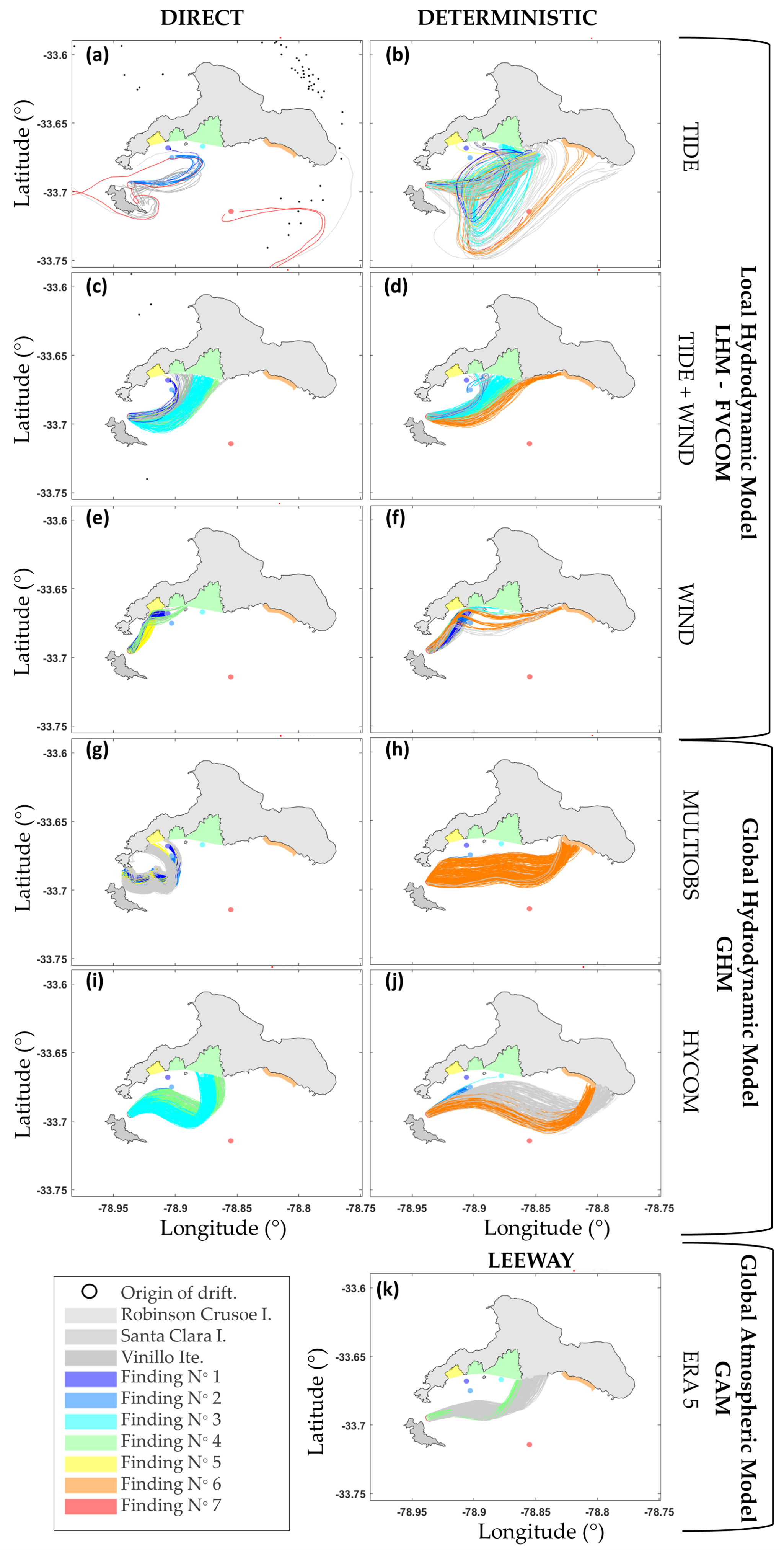
3.3. Qualitative Performance

The qualitative performance (Figure 15) was conducted by evaluating whether modeled trajectories arrived in the areas where findings were detected during the SAR emergency (Figure 1a). The results from the GHMs show a tendency towards the polygons located in the center and west of the Robinson Crusoe Island. In contrast, the arrivals moved towards the polygons located to the east of the island for the case of deterministic modeling approach (Figure 15). The LEEWAY method showed drift trajectories towards the polygons in center and east of the island (Figure 15), with little success in arriving at the highlighted polygons. The scenarios obtained by LHM exhibited a more varied distribution of arrivals and showed an orientation towards the center and east of the island, but they covered a greater number of intermediate coastal areas (Figure 15).
The analyses considering the arrival to targeted polygons (Figure 15) showed better results for the FVCOM Deterministic Tide model (seven polygons), followed by FVCOM Tide + Direct Wind and FVCOM Deterministic Wind (six polygons each), and FVCOM Tide + Deterministic Wind (five polygons). The rest of the modeling scenarios exhibited arrivals in no more than four polygons. The application of the deterministic method resulted in an improved distribution of the arrivals in most of the cases executed with FVCOM, increasing the spatial distribution of arrivals and, in some cases, increasing the number of arrivals in the target polygons, particularly for the case of FVCOM Tide.

4. Summary and Discussion

This work analyzed particle trajectories modeled using surface currents information from global (HYCOM, MULTIOBS) and local models (FVCOM), and global wind velocity reanalysis data (ERA5). The velocities extracted from these models were imposed directly (e.g., [51,52,53]) and deterministically on the floating element, where the latter solves the horizontal drag force balance considering the effect of winds and ocean currents to obtain the velocity of the floating object (e.g., [20,54,55]). The results represent a cloud of trajectories lagged in space and time, modeled under scenarios that consider different sets of forcing conditions. Particle trajectories were also estimated using the LEEWAY method based on coefficients tabulated by Allen [42] and wind data from the GAM ERA5. All modeled trajectories were compared to drifter trajectories measured during the SAR emergency. We estimated model performance using the existing NCLS index [9,47] and propose a modification of this index termed NCLS m o d . This index modifies the NCLS to include trajectory orientation.
The methodology proposed in the present study includes several aspects that need discussion due to the application of various data sources and trajectory estimation methodologies. The difference in the estimated performance is the sum of errors associated with the numerical modeling, simplifications associated with data interpolation in the force balance used in the deterministic method, the assumption of spatiotemporal lags, and the explicit approximation for the ODE resolution of particle trajectory. To better understand the error proportions in performance calculations, we can assume that the error associated with solving ODEs though the Runge–Kutta’s algorithm [40], the error associated with data interpolation, and the error induced by the spatiotemporal lags were proportional for all the studied scenario, as they were used equally in each case. Similarly, the error associated with simplifications included in the deterministic method calculations [20] was proportional in all scenarios where the methodology was used. However, it may have induced differences with respect to estimation of trajectories using the direct method. Thus, the cause of differences in the modeled trajectories may be separated in two levels: first, the data sources used to derive the hydrodynamics, and second, the method used for trajectory estimation in the MPDE.
For a proper interpretation of results, the local conditions where drifters were released need to be considered. The area between Santa Clara Island and Robinson Crusoe Island is characterized by currents that reverse with the tide, with flood currents towards the southeast and ebb currents towards the northwest when winds speeds are <7 km/h. In contrast, when winds are greater than 7 km/h and persistent from the northwest, the surface current shows a predominant direction towards the southeast [24]. The reversible nature of currents in the channel between the islands was captured by the scenarios modeled with FVCOM forced with Tide and Tide + Wind, which were reflected in both the qualitative and quantitative performance analyses. However, on 14 September, FVCOM was outperformed by the MULTIOBS model; the wind influence was greater that day, reaching intensities of 18.7 km/h from the northwest and influencing drifter trajectories as they showed a southeast movement instead of towards the west. The FVCOM Wind scenario provided results that were very close to those obtained using MULTIOBS, which suggests that a suite of different forcing scenarios in FVCOM (Tide, Wind+Tide, and Wind) are able to capture the local conditions in the area. We note that on 14 September, the LEEWAY method had its best performances. The main disadvantage of this method is the need to associate it with a particular floating element [52,56], which is unknown at first or may not have tabulated parameters (as in the present study).
Due to orographic effects and complex wind patterns, the area between Santa Clara Island and Robinson Crusoe Island develops atmospheric instabilities, strong turbulence, and vertical flows that can change in short time periods and may have caused the plane accident [25]. These short-lived events are usually not well captured in data from GAM, such as ERA5, due to the limited spatio-temporal resolution of the wind fields, particularly in mountainous and geographically complex areas (e.g., [55,57,58]). This suggests that local winds may have been underestimated in the forcing used in the different modeling scenarios, particularly the wind gusts, which are not represented in the model. Moreover, considering that the maximum width of the Robinson Crusoe Island is approximately 15 km, both the GAM and GHM MULTIOBS do not solve their balances accounting for the orography of the island, and their temporal resolution does not allow the representation the high frequency variability of the winds and the wind gust that exist in the channel area between Santa Clara and Robinson Crusoe Islands. These aspects may be improved by coupling a high-resolution atmospheric model to FVCOM (or another LHM) (e.g., [4,59,60]), by considering adjustments to wind stress used as model input based on Ekman relationships [61] and/or incorporate satellite-derived ocean current data when available [53].
Regarding the use of the deterministic method (e.g., [20]), small differences were observed in terms of the short-term trajectories, but this approach resulted in greater performance in 8 of the 9 assessed drifters on 10 September and in 11 of the 13 drifters assessed on 14 September. In terms of daily means, the deterministic method was used in all of the high-performance cases. The differences obtained using this method were evident in the qualitative trajectory analysis, where there were significant improvements in the results of the LHM scenarios, particularly FVCOM Det. Tide.
Drifter trajectories integrate dynamics across the broad spectrum of spatial and temporal ocean scales [12]. LHMs generally produce mesoscale structures with a greater definition (e.g., [29,62]); however, they may contain small-scale effects that are not present in reality or that are displaced in space or time [9,48,49]. Furthermore, high-resolution models may create much more energetic dynamics than coarser scale models, which increases the distance traveled by particles and their dispersion (e.g., [9]). Although both the LHM and the GHM used here classify as "eddy-resolving" models due to their horizontal resolution (e.g., [51]), differences are clear in terms of the dispersion of modeled trajectories (Figure 14); drifter dispersion is much greater in trajectories from the LHM. This is consistent with results from Döös et al. [51], who found that the drifter dispersion rate decreases with increasing model grid resolution. The scale effect was counteracted by introducing a spatio-temporal lag at the start of each modeled trajectory; however, the results for all lagged trajectories were coherent with the best performance trajectory, which suggests that the scale of the spatio-temporal lag is of secondary importance to modeled trajectories. This is in contrast to the results of Amemou et al. [63], who found a first-order effect of the scale of the spatio-temporal lag on trajectory performance. The presence of mesoscale structures can only be evaluated through the measurement of drifter trajectories and the estimation of performance measures such as NCLS and NCLS m o d . Consequently, drifter deployments become a valuable source of information in these types of emergencies.
The numerical modeling of drifter trajectories requires an accurate prediction of near-surface processes that influence current velocities in the upper ocean layer; while these processes may be dominated by wind stress at open sea and the inner shelf (e.g., [64,65]), surface waves and processes related to depth-limited wave breaking become relevant in nearshore areas (e.g., [66,67]). Carniel et al. [68] showed that including the wave breaking process in modeling the trajectory of surface drifters improved the accuracy of the simulation by up to 25 % . Similarly, Tang et al. [54] studied wave effects on modeling ocean surface currents, concluded that the wave-driven Stokes drift increased surface drift speeds by 35 % and that the inclusion of wave effects improved simulations significantly. Wave-breaking effects are not included in our LHM; however, we do not expect these processes to influence our quantitative performance analysis notably as trajectories mostly occur in deep waters where depth-limited wave breaking is absent. It may be argued that not including wave effects may affect our qualitative performance assessment, as we evaluated arrivals to polygons located at the coast of the islands. In these regions, wave-driven currents may be relevant and may transport materials along the coast depending on the direction of the incident wave field (e.g., [69]). Future work considers the incorporation of wave dynamics into the LHM [70].

Author Contributions

Conceptualization, P.C. and R.P.F.; methodology, P.C.; software, P.C.; validation, P.C.; formal analysis, P.C.; investigation, P.C.; resources, P.C.; data curation, P.C.; writing—original draft preparation, P.C. and R.P.F.; writing—review and editing, P.C. and R.P.F. All authors have read and agreed to the published version of the manuscript.

Funding

This research received no external funding.

Institutional Review Board Statement

Not applicable.

Informed Consent Statement

Not applicable.

Data Availability Statement

Not applicable.

Acknowledgments

We thank the Chilean Navy, the Chilean Air Force, and the Chilean Meteorological Service for providing the data collected during the emergency. We especially acknowledge the Hydrographic and Oceanographic Service (SHOA) for providing atmospheric and oceanographic data. We also thank Elías Ovalle and Daniel Brieva at the CHIOOS observatory for their support with FVCOM modeling. P.C. acknowledges support from the Graduate School at Universidad Técnica Federico Santa María.

Conflicts of Interest

The authors declare no conflict of interest.

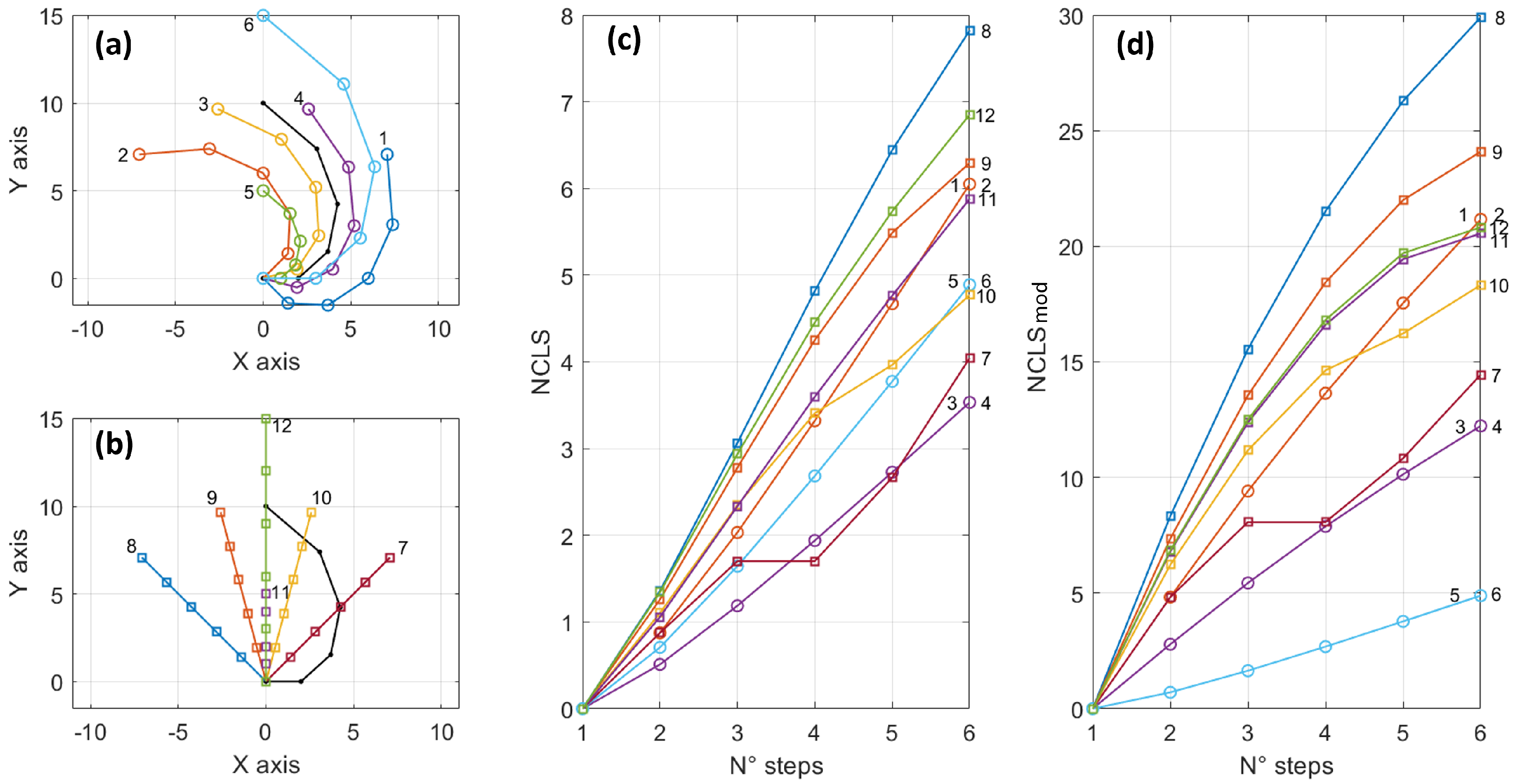
Appendix A. Mathematical Test of NCLS and NCLS mod Indices

Figure A1 compares the use of the standard NCLS and the NCLS m o d indices in evaluating the performance of several artificial trajectories (trajectories from 1 to 12) with respect to a curved trajectory (trajectory 0). We analyzed curved trajectories displaced ± 45 ° compared to trajectory 0 (trajectories 1 and 2), displaced ± 15 ° compared to trajectory 0 (trajectories 3 and 4) and without angular displacement, but with a path of ± 50 % compared to trajectory 0 (trajectories 5 and 6). We also analyzed straight trajectories, with constant angular deviation of ± 45 ° (trajectories 7 and 8), with constant angular deviation ± 15 ° (trajectories 9 and 10), and without angular displacements, but with a path of ± 50 % compared to trajectory 0 (trajectories 11 and 12). We observe that the NCLS m o d index, unlike NCLS, privileges trajectories with a greater angular performance (trajectories 5 and 6), over those of lower D i . Thus, trajectories 7 and 10, which were in third and fourth place according to NCLS, are now moved to positions seven and eight. The latter is also observed when NCLS m o d positions trajectories 11 and 12 with better performance than trajectories 1, 2, 8 and 9.
Figure A1. Comparison between NCLS and NCLS m o d through artificial trajectories. (a) Artificial curved trajectories; (b) straight artificial trajectories; (c) estimated performance through NCLS; and (d) estimated performance through NCLS m o d .
Jmse 10 01649 g0a1

Appendix B. Statistic Performance Result of Quantitative Analyses of Trajectories

Table A1. Performance statistic values for each model and scenario used for 10 September 2011.
Best NCLS mod Trajectory
ModelNCLS mod Angle [°]PathNCLS
FinalMeanSTDFinalMeanSTDDifference (m)[46]
FVC T2.8501.7080.82533.323.39.4602.42.713
FVC T Det.2.7141.5990.78332.523.18.9562.42.582
FVC T + W2.9211.7210.83735.223.910.5674.42.779
FVC T + W Det2.8411.7580.80132.524.09.9605.12.697
FVC W4.4052.8541.18258.158.612.9999.64.072
FVC W Det.4.2252.6981.14952.349.715.21029.13.946
HYCOM4.9323.0031.33387.367.419.71122.24.534
HYCOM Det.4.9082.9881.31584.065.716.81046.44.516
MULTIOBS4.1302.5071.13854.038.215.01101.53.893
MULTIOBS Det.4.1432.6251.06751.641.412.31049.53.886
LEEWAY4.5422.6551.26669.642.819.31199.84.267
Mean of All Trajectories
ModelNCLS mod Angle [°]PathNCLS
FinalMeanSTDFinalMeanSTDDifference (m)[46]
FVC T5.2383.4881.73671.669.134.9661.54.795
FVC T Det.5.2233.4751.75071.668.934.6639.64.781
FVC T + W5.3023.5321.74071.869.834.7663.84.855
FVC T + W Det5.2903.5181.74871.769.534.3642.44.844
FVC W6.1334.2391.588106.4113.733.91108.25.467
FVC W Det.6.0794.1941.595106.3112.835.91129.25.415
HYCOM5.5383.6711.28799.891.921.91131.24.995
HYCOM Det.5.5313.6421.28397.889.220.81080.25.001
MULTIOBS5.6313.7241.40494.790.838.81159.65.078
MULTIOBS Det.5.6203.6921.39394.088.635.91119.15.078
LEEWAY5.3163.4831.27388.078.726.01254.04.833
Table A2. Performance statistic values for each model and scenario used for 14 September 2011.
Best NCLS mod Trajectory
ModelNCLS mod Angle [°]PathNCLS
FinalMeanSTDFinalMeanSTDDifference (m)[46]
FVC T3.4812.1610.92942.039.46.3934.23.183
FVC T Det.3.3412.1520.86042.640.56.3888.83.010
FVC T + W3.4052.2140.85242.039.85.9909.93.097
FVC T + W Det3.2942.1340.84639.339.16.4892.82.992
FVC W3.3572.1010.90232.831.16.61012.23.158
FVC W Det.3.0131.9080.82125.025.66.61006.02.878
HYCOM3.6772.1481.05842.733.29.21069.23.455
HYCOM Det.3.5312.0661.01641.532.78.5994.13.310
MULTIOBS2.4791.5540.68412.510.44.3947.92.411
MULTIOBS Det.2.4031.4930.66914.611.64.4898.12.320
LEEWAY3.3371.9610.95036.627.28.41046.03.158
Mean of All Trajectories
ModelNCLS mod Angle [°]PathNCLS
FinalMeanSTDFinalMeanSTDDifference (m)[46]
FVC T6.3184.0911.917112.0112.536.7870.65.572
FVC T Det.6.1293.9651.880107.7108.136.2849.95.417
FVC T + W6.1473.9811.894108.6109.037.4876.95.425
FVC T + W Det5.9843.8691.856104.7104.936.7855.15.293
FVC W4.8943.2331.26568.575.128.81103.44.382
FVC W Det.4.5473.0271.19558.266.529.61124.74.115
HYCOM4.5342.8831.16060.860.222.61113.44.119
HYCOM Det.4.5072.8451.15459.458.219.41055.44.107
MULTIOBS3.6732.4441.05039.142.930.71090.73.387
MULTIOBS Det.3.6082.3861.02140.242.727.31043.93.329
LEEWAY4.2202.6911.08952.451.921.51095.63.865

References

  1. National Search and Rescue Manual; Technical Report; Australian Maritime Safety Authority: Canberra, Australia, 2022.
  2. COSPAS-SARSAT. Technical Report Nº47; Technical Report; Secretariat of the International Cospas-Sarsat Programme: Monteréal, QC, Canada, 2021. [Google Scholar]
  3. International Aeronautical and Maritime Rescue Manual; International Maritime Organization: London, UK; International Civil Aviation Organization: Montreal, QC, Canada, 2019.
  4. Chen, C.; Limeburner, R.; Gao, G.; Xu, Q.; Qi, J.; Xue, P.; Lai, Z.; Lin, H.; Beardsley, R.; Owens, B.; et al. FVCOM model estimate of the location of Air France 447. Ocean Dyn. 2012, 62, 943–952. [Google Scholar] [CrossRef]
  5. Chen, C.; Liu, H.; Beardsley, R.C. An unstructured grid, finite-volume, three-dimensional, primitive equations ocean model: Application to coastal ocean and estuaries. J. Atmos. Ocean. Technol. 2003, 20, 159–186. [Google Scholar] [CrossRef]
  6. Skamarock, W.C.; Klemp, J.B.; Dudhia, J.; Gill, D.O.; Barker, D.M.; Wang, W.; Powers, J.G. A Description of the Advanced Research WRF Version 3. NCAR Technical Note-475+STR; National Center for Atmospheric Research: Boulder, CO, USA, 2008. [Google Scholar]
  7. Cho, K.H.; Li, Y.; Wang, H.; Park, K.S.; Choi, J.Y.; Shin, K.I.; Kwon, J.I. Development and validation of an operational search and rescue modeling system for the Yellow Sea and the East and South China Seas. J. Atmos. Ocean. Technol. 2014, 31, 197–215. [Google Scholar] [CrossRef]
  8. Campuzano, F.; Brito, D.; Juliano, M.; Fernandes, R.; de Pablo, H.; Neves, R. Coupling watersheds, estuaries and regional ocean through numerical modelling for Western Iberia: A novel methodology. Ocean Dyn. 2016, 66, 1745–1756. [Google Scholar] [CrossRef]
  9. Révelard, A.; Reyes, E.; Mourre, B.; Hernández-Carrasco, I.; Rubio, A.; Lorente, P.; Fernández, C.D.L.; Mader, J.; Álvarez-Fanjul, E.; Tintoré, J. Sensitivity of Skill Score Metric to Validate Lagrangian Simulations in Coastal Areas: Recommendations for Search and Rescue Applications. Front. Mar. Sci. 2021, 8, 630388. [Google Scholar] [CrossRef]
  10. Artale, V.; Boffetta, G.; Celani, A.; Cencini, M.; Vulpiani, A. Dispersion of passive tracers in closed basins: Beyond the diffusion coefficient. Phys. Fluids 1997, 9, 3162–3171. [Google Scholar] [CrossRef] [Green Version]
  11. Aurell, E.; Boffetta, G.; Crisanti, A.; Paladin, G.; Vulpiani, A. Predictability in the large: An extension of the concept of Lyapunov exponent. J. Phys. A Math. Gen. 1997, 30, 1–26. [Google Scholar] [CrossRef] [Green Version]
  12. Haza, A.C.; Griffa, A.; Martin, P.; Molcard, A.; Özgökmen, T.M.; Poje, A.C.; Barbanti, R.; Book, J.W.; Poulain, P.M.; Rixen, M.; et al. Model-based directed drifter launches in the Adriatic Sea: Results from the DART experiment. Geophys. Res. Lett. 2007, 34. [Google Scholar] [CrossRef] [Green Version]
  13. Haza, A.C.; Poje, A.C.; Özgökmen, T.M.; Martin, P. Relative dispersion from a high-resolution coastal model of the Adriatic Sea. Ocean Model. 2008, 22, 48–65. [Google Scholar] [CrossRef]
  14. Shadden, S.C.; Lekien, F.; Marsden, J.E. Definition and properties of Lagrangian coherent structures from finite-time Lyapunov exponents in two-dimensional aperiodic flows. Phys. D Nonlinear Phenom. 2005, 212, 271–304. [Google Scholar] [CrossRef]
  15. Serra, M.; Sathe, P.; Rypina, I.; Kirincich, A.; Ross, S.D.; Lermusiaux, P.; Allen, A.; Peacock, T.; Haller, G. Search and rescue at sea aided by hidden flow structures. Nat. Commun. 2020, 11, 1–7. [Google Scholar] [CrossRef] [PubMed]
  16. Muller-Karger, F.; Roffer, M.; Walker, N.; Oliver, M.; Schofield, O.; Abbott, M.; Graber, H.; Leben, R.; Goni, G. Satellite remote sensing in support of an integrated ocean observing system. IEEE Geosci. Remote Sens. Mag. 2013, 1, 8–18. [Google Scholar] [CrossRef]
  17. Le Traon, P.Y.; Reppucci, A.; Alvarez Fanjul, E.; Aouf, L.; Behrens, A.; Belmonte, M.; Bentamy, A.; Bertino, L.; Brando, V.E.; Kreiner, M.B.; et al. From observation to information and users: The Copernicus Marine Service perspective. Front. Mar. Sci. 2019, 6, 234. [Google Scholar] [CrossRef] [Green Version]
  18. Sotillo, M.G. Ocean Modelling in Support of Operational Ocean and Coastal Services. J. Mar. Sci. Eng. 2022, 10, 1482. [Google Scholar] [CrossRef]
  19. Hufford, G.; Broida, S. Estimation of the leeway drift of small craft. Ocean Eng. 1976, 3, 123–132. [Google Scholar] [CrossRef]
  20. Di Maio, A.; Martin, M.V.; Sorgente, R. Evaluation of the search and rescue LEEWAY model in the Tyrrhenian Sea: A new point of view. Nat. Hazards Earth Syst. Sci. 2016, 16, 1979–1997. [Google Scholar] [CrossRef] [Green Version]
  21. Chassignet, E.P.; Hurlburt, H.E.; Metzger, E.J.; Smedstad, O.M.; Cummings, J.A.; Halliwell, G.R.; Bleck, R.; Baraille, R.; Wallcraft, A.J.; Lozano, C.; et al. US GODAE: Global ocean prediction with the HYbrid Coordinate Ocean Model (HYCOM). Oceanography 2009, 22, 64–75. [Google Scholar] [CrossRef] [Green Version]
  22. Rio, M.H.; Mulet, S.; Picot, N. Beyond GOCE for the ocean circulation estimate: Synergetic use of altimetry, gravimetry, and in situ data provides new insight into geostrophic and Ekman currents. Geophys. Res. Lett. 2014, 41, 8918–8925. [Google Scholar] [CrossRef]
  23. Hersbach, H.; Bell, B.; Berrisford, P.; Hirahara, S.; Horányi, A.; Muñoz-Sabater, J.; Nicolas, J.; Peubey, C.; Radu, R.; Schepers, D.; et al. The ERA5 global reanalysis. Q. J. R. Meteorol. Soc. 2020, 146, 1999–2049. [Google Scholar] [CrossRef]
  24. Derrotero de la Costa de Chile. Volumen I. De Arica a Canal Chacao; Technical Report; Hydrographic and Oceanographic Service of the Chilean Navy: Valparaíso, Chile, 2013.
  25. Gracia, L. Links for a successful investigation: C-212 Robinson Crusoe Island Accident Case. Airbus Def. Space. Mil. Aircr. 2017, 1–12. Available online: https://www.isasi.org/Documents/library/technical-papers/2016/Thurs/Gracia_C212RobisonCrusoe.pdf (accessed on 15 September 2022).
  26. Hunke, E.; Lipscomb, W. The Los Alamos Sea Ice Model Documentation and Software User’s Manual, Version 4.1; National Center for Atmospheric Research: Boulder, CO, USA, 2010. Available online: https://csdms.colorado.edu/w/images/CICE_documentation_and_software_user’s_manual.pdf(accessed on 15 September 2022).
  27. Cowles, G.W. Parallelization of the FVCOM coastal ocean model. Int. J. High Perform. Comput. Appl. 2008, 22, 177–193. [Google Scholar] [CrossRef]
  28. Shore, J.A. Modelling the circulation and exchange of Kingston Basin and Lake Ontario with FVCOM. Ocean Model. 2009, 30, 106–114. [Google Scholar] [CrossRef]
  29. Qu, K.; Tang, H.; Agrawal, A.; Jiang, C.; Deng, B. Evaluation of SIFOM-FVCOM system for high-fidelity simulation of small-scale coastal ocean flows. J. Hydrodyn. 2016, 28, 994–1002. [Google Scholar] [CrossRef]
  30. Guerra, M.; Cienfuegos, R.; Thomson, J.; Suarez, L. Tidal energy resource characterization in Chacao Channel, Chile. Int. J. Mar. Energy 2017, 20, 1–16. [Google Scholar] [CrossRef]
  31. Olson, C.J.; Becker, J.J.; Sandwell, D.T. A new global bathymetry map at 15 arcsecond resolution for resolving seafloor fabric: SRTM15_PLUS. In AGU Fall Meeting Abstracts; American Geophysical Union: San Francisco, CA, USA, 2014; Volume 2014, p. OS34A-03. [Google Scholar]
  32. Engwirda, D. Locally Optimal Delaunay-Refinement and Optimisation-Based Mesh Generation. Ph.D. Thesis, The University of Sydney, Sydney, Australia, 2014. [Google Scholar]
  33. Chen, C.; Beardsley, R.; Cowles, G.; Qi, J.; Lai, Z.; Gao, G.; Stuebe, D.; Xu, Q.; Xue, P.; Ge, J.; et al. An Unstructured-Grid, Finite-Volume Community Ocean Model: FVCOM User Manual; Sea Grant College Program; Massachusetts Institute of Technology: Cambridge, MA, USA, 2012. [Google Scholar]
  34. Atlas Oceanográfico de Chile (18°21′ S a 50°00′ S) Volumen 1; Technical Report; Hydrographic and Oceanographic Service of the Chilean Navy: Valparaíso, Chile, 1996.
  35. Egbert, G.D.; Erofeeva, S.Y. Efficient inverse modeling of barotropic ocean tides. J. Atmos. Ocean. Technol. 2002, 19, 183–204. [Google Scholar] [CrossRef]
  36. Instrucciones Oceanográficas Nº 2: Método Oficial Para el Cálculo de los Valores No Armónicos de la Marea; Technical Report; Hydrographic and Oceanographic Service of the Chilean Navy: Valparaíso, Chile, 1999.
  37. Lai, Z. A Non-Hydrostatic Unstructured-Grid Finite-Volume Coastal Ocean Model System (fvcom-nh): Development, Validation and Application: A Dissertation in Marine Science and Technology. Ph.D. Thesis, University of Massachusetts, North Dartmouth, MA, USA, 2009. [Google Scholar]
  38. Mellor, G.L.; Yamada, T. Development of a turbulence closure model for geophysical fluid problems. Rev. Geophys. 1982, 20, 851–875. [Google Scholar] [CrossRef] [Green Version]
  39. Grant, W.; Madsen, O. Combined Wave and Current Interaction with a Rough Bottom. J. Geophys. Res. Atmos. 1979, 84, 1797–1808. [Google Scholar] [CrossRef]
  40. Celia, M.A.; Gray, W.G. Numerical Methods for Differential Equations: Fundamental Concepts for Scientific and Engineering Applications; Pearson College Division: Engelwood Cliffs, NJ, USA, 1992. [Google Scholar]
  41. Kundu, P.K.; Cohen, I.M.; Dowling, D.R. Fluid Mechanics; Academic Press: Cambridge, MA, USA, 2015. [Google Scholar]
  42. Allen, A.A. Leeway Divergence; Technical Report; U.S. Coast Guard Research and Development Center: Groton, CT, USA, 2005. [Google Scholar]
  43. Sayol, J.; Orfila, A.; Simarro, G.; Conti, D.; Renault, L.; Molcard, A. A Lagrangian model for tracking surface spills and SaR operations in the ocean. Environ. Model. Softw. 2014, 52, 74–82. [Google Scholar] [CrossRef] [Green Version]
  44. Allen, A.A.; Plourde, J.V. Review of Leeway: Field Experiments and Implementation; Technical Report; U.S. Coast Guard Research and Development Center: Groton, CT, USA, 1999. [Google Scholar]
  45. Ohlmann, J.; Romero, L.; Pallàs-Sanz, E.; Perez-Brunius, P. Anisotropy in coastal ocean relative dispersion observations. Geophys. Res. Lett. 2019, 46, 879–888. [Google Scholar] [CrossRef]
  46. Hoerner, S.F. Fluid-Dynamic Drag: Practical Information on Aerodynamic Drag and Hydrodynamic Resistance; Hoerner Fluid Dynamics: Brick Town, NJ, USA, 1965. [Google Scholar]
  47. Liu, Y.; Weisberg, R.H. Evaluation of trajectory modeling in different dynamic regions using normalized cumulative Lagrangian separation. J. Geophys. Res. Ocean. 2011, 116, C09013. [Google Scholar] [CrossRef] [Green Version]
  48. Sperrevik, A.K.; Röhrs, J.; Christensen, K.H. Impact of data assimilation on E ulerian versus L agrangian estimates of upper ocean transport. J. Geophys. Res. Ocean. 2017, 122, 5445–5457. [Google Scholar] [CrossRef]
  49. Mourre, B.; Aguiar, E.; Juza, M.; Hernandez-Lasheras, J.; Reyes, E.; Heslop, E.; Escudier, R.; Cutolo, E.; Ruiz, S.; Mason, E.; et al. Assessment of high-resolution regional ocean prediction systems using multi-platform observations: Illustrations in the western Mediterranean Sea. New Front. Oper. Oceanogr. 2018, 663–694. [Google Scholar] [CrossRef] [Green Version]
  50. Aguiar, E.; Mourre, B.; Juza, M.; Reyes, E.; Hernández-Lasheras, J.; Cutolo, E.; Mason, E.; Tintoré, J. Multi-platform model assessment in the Western Mediterranean Sea: Impact of downscaling on the surface circulation and mesoscale activity. Ocean Dyn. 2020, 70, 273–288. [Google Scholar] [CrossRef] [Green Version]
  51. Döös, K.; Rupolo, V.; Brodeau, L. Dispersion of surface drifters and model-simulated trajectories. Ocean Model. 2011, 39, 301–310. [Google Scholar] [CrossRef]
  52. Brushett, B.A.; Allen, A.A.; King, B.A.; Lemckert, C.J. Application of leeway drift data to predict the drift of panga skiffs: Case study of maritime search and rescue in the tropical pacific. Appl. Ocean Res. 2017, 67, 109–124. [Google Scholar] [CrossRef]
  53. Dagestad, K.F.; Röhrs, J. Prediction of ocean surface trajectories using satellite derived vs. modeled ocean currents. Remote Sens. Environ. 2019, 223, 130–142. [Google Scholar] [CrossRef]
  54. Tang, C.L.; Perrie, W.; Jenkins, A.D.; DeTracey, B.M.; Hu, Y.; Toulany, B.; Smith, P.C. Observation and modeling of surface currents on the Grand Banks: A study of the wave effects on surface currents. J. Geophys. Res. Ocean. 2007, 112. [Google Scholar] [CrossRef]
  55. Zhang, J.; Teixeira, Â.P.; Soares, C.G.; Yan, X. Probabilistic modelling of the drifting trajectory of an object under the effect of wind and current for maritime search and rescue. Ocean Eng. 2017, 129, 253–264. [Google Scholar] [CrossRef]
  56. Breivik, Ø.; Allen, A.A. An operational search and rescue model for the Norwegian Sea and the North Sea. J. Mar. Syst. 2008, 69, 99–113. [Google Scholar] [CrossRef] [Green Version]
  57. Minola, L.; Zhang, F.; Azorin-Molina, C.; Pirooz, A.; Flay, R.; Hersbach, H.; Chen, D. Near-surface mean and gust wind speeds in ERA5 across Sweden: Towards an improved gust parametrization. Clim. Dyn. 2020, 55, 887–907. [Google Scholar] [CrossRef]
  58. Aksamit, N.O.; Sapsis, T.; Haller, G. Machine-Learning Mesoscale and Submesoscale Surface Dynamics from Lagrangian Ocean Drifter Trajectories. J. Phys. Oceanogr. 2020, 50, 1179–1196. [Google Scholar] [CrossRef]
  59. Jiang, Y.; Han, S.; Shi, C.; Gao, T.; Zhen, H.; Liu, X. Evaluation of HRCLDAS and ERA5 datasets for near-surface wind over hainan island and south China sea. Atmosphere 2021, 12, 766. [Google Scholar] [CrossRef]
  60. Li, S.; Chen, C. Air-sea interaction processes during hurricane Sandy: Coupled WRF-FVCOM model simulations. Prog. Oceanogr. 2022, 206, 102855. [Google Scholar] [CrossRef]
  61. Edwards, K.; Werner, F.; Blanton, B. Comparison of observed and modeled drifter trajectories in coastal regions: An improvement through adjustments for observed drifter slip and errors in wind fields. J. Atmos. Ocean. Technol. 2006, 23, 1614–1620. [Google Scholar] [CrossRef]
  62. Bellafiore, D.; Umgiesser, G. Hydrodynamic coastal processes in the North Adriatic investigated with a 3D finite element model. Ocean Dyn. 2010, 60, 255–273. [Google Scholar] [CrossRef]
  63. Amemou, H.; Koné, V.; Aman, A.; Lett, C. Assessment of a Lagrangian model using trajectories of oceanographic drifters and fishing devices in the Tropical Atlantic Ocean. Prog. Oceanogr. 2020, 188, 102426. [Google Scholar] [CrossRef]
  64. Austin, J.A.; Lentz, S.J. The inner shelf response to wind-driven upwelling and downwelling. J. Phys. Oceanogr. 2002, 32, 2171–2193. [Google Scholar] [CrossRef]
  65. Fewings, M.; Lentz, S.J.; Fredericks, J. Observations of cross-shelf flow driven by cross-shelf winds on the inner continental shelf. J. Phys. Oceanogr. 2008, 38, 2358–2378. [Google Scholar] [CrossRef] [Green Version]
  66. Battjes, J.A.; Sobey, R.J.; Stive, M. Nearshore circulation. In Manuscript for “The Sea” The Sea, Volume 9: Ocean Engineering Science; Harvard University Press: Cambridge, MA, USA, 1990. [Google Scholar]
  67. Lentz, S.; Fewings, M. The wind-and wave-driven inner-shelf circulation. Annu. Rev. Mar. Sci. 2012, 4, 317–343. [Google Scholar] [CrossRef] [Green Version]
  68. Carniel, S.; Warner, J.C.; Chiggiato, J.; Sclavo, M. Investigating the impact of surface wave breaking on modeling the trajectories of drifters in the northern Adriatic Sea during a wind-storm event. Ocean Model. 2009, 30, 225–239. [Google Scholar] [CrossRef]
  69. Thornton, E.B.; Guza, R. Surf zone longshore currents and random waves: Field data and models. J. Phys. Oceanogr. 1986, 16, 1165–1178. [Google Scholar] [CrossRef]
  70. Chen, T.; Zhang, Q.; Wu, Y.; Ji, C.; Yang, J.; Liu, G. Development of a wave-current model through coupling of FVCOM and SWAN. Ocean Eng. 2018, 164, 443–454. [Google Scholar] [CrossRef]
Figure 1. Study area and drifter deployments. (a) Juan Fernández Archipelago. Colored areas indicate locations where accident remains were found. (b) Geographic location of drifter deployments on 10 September (magenta triangles) and 14 September (green triangles) 2011.
Jmse 10 01649 g001
Figure 2. Process flow of the modeling scheme, including the data sources, hydrodynamic models, trajectory estimation methods, and operational products.
Jmse 10 01649 g002
Figure 3. Unstructured triangular grid used for FVCOM modeling. (a) Model domain. Boundary and sponge nodes are indicated as dark and light-gray circles, respectively. (b) Zoom-in to the Juan Fernández Archipelago region. RCI: Robinson Crusoe Island.
Jmse 10 01649 g003
Figure 4. Open boundary forcings incorporated into FVCOM. (a,b) TPXO tidal model and measured tidal elevation at Cumberland Bay (SHOA), (c,d) Interpolated U wind component from ERA5 and measured U wind speed at Cumberland Bay station (DGAC). (e,f) Interpolated V wind component from ERA5 and measured V wind speed at Cumberland Bay station (DGAC).
Jmse 10 01649 g004
Figure 5. Diagram of drifters released by SHOA (10 and 14 September 2011).
Jmse 10 01649 g005
Figure 6. Diagram of NCLS m o d calculation. L o b s : path of the observed drifted; L m o d : path of the modeled drifted; D: distance between modeled and observed drift; and α : the angle formed between L o b s , L m o d and the origin.
Jmse 10 01649 g006
Figure 7. Comparison between sea level time series of at Cumberland Bay (SHOA) and model output of FVCOM Tide + Wind. (a) Compared time series and (b) correlation analysis.
Jmse 10 01649 g007
Figure 8. Drifter travel distance modeled by FVCOM (green and blue lines). The solid black line indicated the reference distance. Dashed lines indicate mean traveled distance for the cases indicated in the legend.
Jmse 10 01649 g008
Figure 9. Drifter measurement periods during 10 September 2011 (a) and 14 September 2011 (b).
Jmse 10 01649 g009
Figure 10. Geographic comparison between measured and modeled drifters with best NCLS m o d for 10 September 2011. (ai) Drifter deployments 1–9, respectively, as indicated in Figure 9a. Panel titles indicate drifter deployment number (X-D10, where X is drifter number). FVC = FVCOM; T = Tide; W = Wind; Det. = deterministic (drag force) method.
Jmse 10 01649 g010
Figure 11. Geographic comparison between measured and modeled drifters with best NCLS m o d for 14 September 2011. (am) Drifter deployments 1–13, respectively, as indicated in Figure 9b. Panel titles indicate drifter deployment number (X-D14, where X is drifter number). FVC = FVCOM; T = Tide; W = Wind; Det. = deterministic (drag force) method.
Jmse 10 01649 g011
Figure 12. Time evolution of NCLS m o d values during 10 September 2011. (ai) Drifter deployments 1–9, respectively, as indicated in Figure 9a. Panel titles indicate drifter deployment number (X-D10, where X is drifter number). FVC = FVCOM; T = Tide; W = Wind; Det. = deterministic (drag force) method.
Jmse 10 01649 g012
Figure 13. Time evolution of NCLS m o d values during 14 September 2011. (am) Drifter deployments 1–13, respectively, as indicated in Figure 9b. Panel titles indicate drifter deployment number (X-D14, where X is drifter number). FVC = FVCOM; T = Tide; W = Wind; Det. = deterministic (drag force) method.
Jmse 10 01649 g013
Figure 14. Zoomed-in trajectory of drifter 8 on 10 September 2011. FVC = FVCOM; T = Tide; W = Wind; Det. = deterministic (drag force) method.
Jmse 10 01649 g014
Figure 15. Particle trajectories between 2 and 8 September 2011 using the LHM, GHM, and LEEWAY methods. (af) LHM method, (gj) GHM method, (k) LEEWAY method. Colored lines indicate trajectories arriving to the locations where accident remains were found, as shown in Figure 1a.
Jmse 10 01649 g015
Publisher’s Note: MDPI stays neutral with regard to jurisdictional claims in published maps and institutional affiliations.

