Article

Accelerating Predictions of Morphological Bed Evolution by Combining Numerical Modelling and Artificial Neural Networks

by
Andreas Papadimitriou
1,2,*,
Michalis Chondros
1,2,
Anastasios Metallinos
1,2 and
Vasiliki Tsoukala
1
1
Laboratory of Harbour Works, School of Civil Engineering, National Technical University of Athens, 15780 Zografou, Greece
2
Scientia Maris, 15234 Chalandri, Greece
*
Author to whom correspondence should be addressed.
J. Mar. Sci. Eng. 2022, 10(11), 1621; https://doi.org/10.3390/jmse10111621
Submission received: 30 September 2022 / Revised: 16 October 2022 / Accepted: 18 October 2022 / Published: 2 November 2022
(This article belongs to the Special Issue Estuaries, Coasts, and Seas in a Changing Climate)

Abstract

:
Process-based models have been employed extensively in the last decades for the prediction of coastal bed evolution in the medium term (1–5 years), under the combined action of waves and currents, due to their ability to resolve the dominant coastal processes. Despite their widespread application, they are associated with high demand for computational resources, rendering the annual prediction of the coastal bed evolution a tedious task. To combat this, wave input reduction methods are generally employed to reduce the sheer amount of sea-states to be simulated to assess the bed level changes. The purpose of this research is to further expand on the concept of input reduction methods by presenting a methodology combining numerical modelling and an Artificial Neural Network (ANN). The trained ANN is tasked with eliminating wave records unable to initiate sediment motion and hence further reduce the required computational times. The methodology was implemented in both an idealized and a real-field case study to examine the sensitivity, and produced very satisfactory predictions of the rates of bed level change, with respect to a benchmark simulation containing a very detailed wave climate. The obtained results have strong implications for further accelerating the demanding morphological simulations while enhancing the reliability and accuracy of model predictions.

1. Introduction

The prediction of coastal bed morphological evolution, and ultimately the shift of the shoreline position under the combined effect of waves and currents, are of high interest to the scientists and the public since coastal erosion has strong implications for environment, economy, and community safety. Typically, process-based models are utilized to carry out this prediction, with each model instance considering different processes and better suited for specific applications of varying temporal and spatial scales. In the presence of coastal structures, to investigate the morphological coastal evolution in a timeframe of 1–10 years, coastal area models [1] are usually employed due to their ability to prescribe in great detail the complex nearshore processes driving sediment transport and the subsequent morphological bed evolution. However, these models are inherently associated with staggering computational burdens, creating the need to speed up the simulations while simultaneously retaining the reliability and accuracy of the results.
To that end, various upscaling techniques have been proposed in the literature aiming to alleviate the computational cost of implementing coastal area models [2,3,4]. Out of these techniques, the one commonly employed by coastal engineers is wave input reduction [5,6,7,8,9], a procedure aiming to reduce the sheer amount of forcing input of the coastal area models by smartly selecting wave representatives able to reproduce the morphological changes induced by the full set of conditions. In the past decades, several studies have been carried out implementing various methods of wave input reduction enabling the simulation of the morphological evolution of coastal features from years to decades [8,9,10,11,12] and thoroughly investigating their performance.
Most input reduction methods are based on the calculation of proxy quantities (e.g., wave energy flux, net sediment transport rate) to select the representative sea-states considered vital in influencing longshore sediment transport. Since these methods divide the wave climate, which usually comprises a time-series of offshore sea-state wave characteristics, namely wave height, period, and mean wave direction, in wave height, and wave directional bins—they are often called binning input reduction methods [9]. The authors in [12] evaluated the performance of the K-Means clustering algorithm as a viable alternative to the binning input reduction methods and examined various enhancements to improve model results. An older, but still widely implemented branch of input reduction considers the estimation of representative or “equivalent” wave characteristics [5,10,11,13] by considering directional bins of fixed size and selecting the representatives by conserving the longshore sediment transport rate over each bin.
Despite their widespread usage and acceptance, the performance of input reduction methods depends on a multitude of parameters [7,8,9] such as the number of representatives, duration of the wave climate, and sequencing of sea states. For relatively mild wave climates, another factor hindering the performance of input reduction methods is the overestimation of the contribution of lowly energetic sea states in shaping the morphological bed evolution. To counteract this, it is common practice to eliminate wave records not exceeding a certain threshold in the wave height [8]. However, this approach is loosely defined and, if the threshold is set too high, can sometimes lead to the deterioration of results [7]. Papadimitriou et al., [14] presented a wave input reduction method incorporating the elimination of sea states considered unable to initiate sediment motion. In their approach, the authors considered the influence of the waves in the stirring of sediments and proposed the use of numerical modelling to estimate wave orbital velocities nearshore.
The scope of this paper is to expand and improve on the concept of input reduction with filtering proposed by [14], presenting a methodology for eliminating sea states considered unable to initiate sediment motion under the combined effect of waves and currents. To expand the applicability range of the methodology, several simulations have been conducted with a parabolic mild slope wave model and a hydrodynamic model, and the results were used to train an Artificial Neural Network (ANN). The trained ANN is then capable of estimating if a combination of offshore sea-state wave characteristics, on a given bed slope and median sediment diameter, can induce significant morphological changes. The proposed methodology was applied and validated in both an idealized and real-field case study and gave very satisfactory results with strong implications on the enhancement of the reliability and accuracy of morphological modelling predictions, with a simultaneous model run-time reduction.

2. Materials and Methods

2.1. Theoretical Aspects

Sediment particles are constantly entrained, transported, and deposited in the bed under the combined effect of waves and currents. Waves are mostly responsible for setting the sediment grains into motion while the currents transport them [15]. Focusing on a predominantly sandy bed and for flows characterized by very small velocities, the grains tend to be generally immovable [16]. As flow velocity gradually increases some sediment entrainment begins to take place hence defining a threshold of sediment motion, firstly analyzed in the classical work of [17]. The most precise measure of the threshold of motion is expressed in terms of the ratio of the force exerted by the bed shear stress acting to move the sand grains on the bed layer, to the submerged weight grain resisting this action. Under combined waves and currents, the maximum value of the bed-shear stress over a wave cycle ( τ max ) is mostly responsible for setting the sediment grains into motion. Many researchers have attempted to describe the non-linear interaction between the wave and current boundary layers [18,19,20], leading to various formulations to compute the value of τ max . In general, it is related to the mean value of the combined bed-shear stress due to waves and currents τ m and the individual contributions of the waves τ w and currents τ c . An approximation to compute τ m considering a two-coefficient fitting to the theoretical models given by [21], reads:
τ m = τ c [ 1 + 1 . 2 ( τ w τ w + τ c ) 3 . 2 ]
where τ m [kg∙m/s2] is the mean bed shear stress over a wave cycle, τ w [kg∙m/s2] is the bed shear stress due to the effect of the waves and τ c [kg∙m/s2] is the current-only bed shear stress contribution.
Waves generate an oscillatory velocity, which obtains its maximum value at the top of the wave boundary layer and is responsible for stirring sediment. The near-bed orbital velocity signal U w can be obtained through the linear wave theory:
U w = π H T   sin h ( kh )
where: H [m] is the wave height of a monochromatic wave, T [s] is the wave period, k [rad/m] is the wavenumber and h [m] is the still water depth.
The bed shear stress due to waves can then be obtained through the following relationship:
τ w = 1 2 ρ f w U w 2
where: ρ [kg/m3] is the water density and fw [-] is the wave friction factor.
The wave friction factor depends on the prevailing hydrodynamic conditions and type of flow, i.e., if it is laminar, smooth, transitional, or rough turbulent and is a function of the relative bed roughness r:
r = U w T 2 π k s
where: ks [-] is the Nikuradse equivalent sand grain roughness usually related to the mean sediment diameter d50.
Inside the surf zone, the conditions are considered to be rough and turbulent and the bed is assumed to be flat. Many formulations exist in the literature (e.g., [16,22]) for the calculation of the wave friction factor. The formula of [16] reads:
f w = 0 . 237 r - 0 . 52
Currents can both stir and transport sediments and as a general principle, the sediment transport generally follows the direction of the current. Assuming a quadratic friction law, the bed shear stress due to currents can be related to the depth-averaged current speed magnitude U ¯ as follows:
τ c = ρ gn 2 h 1 / 3 U ¯ 2
where: n [m1/3/s] is the Manning friction coefficient and g [m/s2] is the acceleration of gravity.
Having distinguished the individual contributions of the waves and currents, the maximum value of the bed shear stress due to the combined effect of waves and currents over a wave cycle can be calculated as shown in [16]:
τ max = [ ( τ m + τ w cos φ ) 2 + ( τ w sin φ ) 2 ] 1 / 2
where φ [rad] is the relative angle between the current and the wave direction.
If the value of τ max exceeds the critical value of the bed shear stress τ cr then sediments are set into motion and transported under the combined effect of waves and currents. The critical value of the bed shear stress is expressed as the ratio of the force exerted by the bed shear stress acting to move the sediment grains on the bed layer, to the submerged weight grain resisting this action and is related to the non-dimensional critical Shields parameter θ cr through the following relationship:
τ cr = θ cr   g   ( ρ s ρ ) d 50
where ρ s [kg/m3] is the density of the sediment grains and d 50 [m] is the median sediment diameter.
An expression to estimate the critical Shields parameter was given by [23]:
θ cr = 0 . 3 1 + 1 . 2 D * + 0 . 055 [ 1   -   e - 0 . 02 D * ]
where D * is the non-dimensional grain diameter given by:
D * = [ g ( s   -   1 ) ν 2 ] 1 / 3 d 50
with g [m/s2] as the acceleration of gravity, s = ρ s ρ w [-] is the ratio of the sediment ( ρ s ) to the water ( ρ w ) density, ν [m2/s] is the kinematic viscosity of the water and d50 [m] is the median sediment diameter.
The aspect of selecting representative wave conditions, able to adequately reproduce the morphological bed evolution obtained by a full set of wave records has been tackled by many researchers over the last decades [8,9,10,14]. As stated previously, the Input Reduction methods utilize quantities responsible for driving the medium-term coastal bed evolution as a proxy to select the set of representative wave characteristics.
Based on this concept, [5] present a method to select annual “equivalent wave characteristics” based on the conservation of the alongshore component of wave energy flux as shown below:
( f i ) H e 2 T e cos a e sin a e , b = ( f i H i 2 T i cos a i sin a i , b )
with H e [m] being the annual equivalent wave height, T e [s] the annual equivalent wave period, and ae [rad] denotes the yearly equivalent incidence wave angle, with the subscript “b” denoting the value at the breaker line. In the right-hand side of Equation (11) the subscript “i” denotes individual wave events, with f i being the frequency of occurrence of each sea-state.
Considering that the wave angles are identical on the right and left-hand side of Equation (11), it can be rewritten as:
H e 2 T e = ( f i T i H i 2 ) f i
The authors in [5], proposed that the “equivalent” wave period T e be estimated through correlation while [11], calculate it as the mean value of each directional bin.
T e = ( f i T i ) f i
The procedure to select a set of annual equivalent wave representatives is as follows: A given dataset of offshore sea state characteristics is divided into an arbitrary number of directional bins at constant intervals. For each directional bin, a set of representative wave characteristics is selected by implementing Equations (12) and (13). The annual equivalent wave incidence angle can be obtained as the mean or the central value in each directional bin.
Based on the above theoretical background, in Section 2.2 a thorough methodology aiming to eliminate sea states that are considered unable to initiate sediment motion and select annual representative wave characteristics will be presented.

2.2. Methodology Outline

Observing Equations (3) and (6)–(8) it can be deduced that the maximum bed shear stress τ max , is a function of the wave characteristics inside the surf zone ( H s , b ,   T p ,   a b ), the wave friction factor f w , the Manning’s coefficient n , the depth-averaged current speed, U ¯ and the bed slope tan β , bottom friction, as well as sediment characteristics. The dependency of τ max to both wave friction factor f w and Manning’s coefficient n can be replaced with a single dependency on the median sediment diameter d50 by specifying a Nikuradse roughness k s = 2 . 5   d 50 . The correspondence between the values within the surf zone and offshore sea-state characteristics H s ,   T p ,   a o can be obtained by implementing a non-linear parabolic mild slope wave model [24] for wave propagation and a flow model to estimate wave-induced current velocities.
However, given an annual dataset of hourly varying offshore sea state wave characteristics, the estimation of τ max would be a tedious task and would require intense computational resources, compromising the acceleration aspect of Input Reduction Methods. Hence, a methodology has been developed in the scope of this research in order to systematically eliminate sea states considered unable to initiate sand motion by combining numerical modelling simulations and the training and implementation of an Artificial Neural Network (ANN) to accelerate morphological modelling simulations and enhance the reliability of model results for a wide application range.
The distinct steps composing the methodology are described below:
  • Three idealized alongshore uniform bathymetries were set up, each characterized by a different value of the bed slope tanβ, namely 1:5, 1:25, and 1:50.
  • Determination of a number of combinations of the Input Parameters (IP) of { H s ,   T p ,   a o ,   d 50 , tan β } to be inserted in the numerical modelling simulations.
It was desirable to define many combinations of the IP in order to cover the wide array of possible values that can be encountered in an arbitrary dataset of offshore sea-state characteristics and coastal bed compositions. Hence, the lower and upper boundaries of the IP were defined and are shown in Table 1, and a Saltelli sampling method [25] typically used in Global Sensitivity Analysis applications, was utilized to obtain a set of 14,168 possible combinations of the IP. To ensure realistic pairs of H s and T p an additional restriction was imposed on the values of the peak wave period, which was to fall within the limits of the Jonswap correlation between H s and T p . To reduce the sheer number of combinations, the widely used K-Means clustering algorithm [26] was implemented to reduce the combinations of the IP to 3000. Additionally, 200 additional scenarios were considered to cover bounding values of the IP raising the final number to 3200.
3.
For each set of IP, nearshore wave propagation simulations were carried out utilizing a spectral version of a nonlinear parabolic mild slope wave model and the resulting radiation stresses were then inserted as forcing input to a flow model based on the depth-averaged Shallow Water Equations, providing the current speed and current direction.
4.
Subsequently calculations of the value of τ max over a wave cycle were carried out for a cross-section in the middle of the domain in the alongshore direction through a post-processing algorithm. The value of τ max is taken as the average value computed shoreward the maximum depth where initiation of breaking occurs, according to the criterion of [27], out of all the 3200 distinct wave records. The set of IP { H s ,   T p ,   a o ,   d 50 , tan β } are consequently linked to a unique value of the Output Parameter (OP) { τ max } . The corresponding values of IP and OP are provided for the training and validation of an ANN, which will predict τ max for any values within the ranges defined in Table 1.
5.
Through Equations (8) and (9) estimation of τ cr follows. Each wave record that satisfies the condition τ max   <   τ cr is eliminated, since it is considered unable to initiate sediment motion and thus produce significant morphological changes. Each eliminated wave record is considered to contribute to the “calm conditions” (i.e., waves from directions exiting the numerical domain) hence it retains its individual frequency of occurrence f i . After elimination, a reduced dataset containing only the sea-states satisfying the Shield’s criterion of incipient sediment motion is obtained.
6.
Utilizing the reduced dataset as input and implementing Equations (12) and (13) a set of annual “equivalent” wave characteristics are defined. The equivalent wave characteristics are used to force the coastal area model and obtain predictions of the coastal bed evolution. In our implementations, we used a combination of a parabolic mild slope wave model (PMS) a hydrodynamic model (HYD), and an initial sedimentation/erosion and morphological model (SDT).
The proposed methodology is valid for real-field conditions (and not for experimental scale) and for any combination of the parameters within the ranges presented in Table 1, considering the combined effect of waves and currents.

2.3. Overview of the Numerical Models

In this section, the governing equations and main features of the numerical models enhanced and implemented in the framework of this methodology are presented. Firstly, a parabolic mild slope wave model was tasked with carrying out wave transformation simulations. A noteworthy aspect of the parabolic approximation of the mild slope equation is that it can be rapidly solved [24] providing fast simulation times which is desirable considering the number of scenarios needed to be simulated for the subsequent training of the ANN. To that end, a highly robust hydrodynamic model based on the depth-averaged Shallow Water Equations (SWE) was utilized for the simulation of the flow field and is presented herein. Additionally, a sediment transport and morphology model was utilized in order to perform the morphological simulations and obtain accretion/erosion rates in the validation of the methodology.

2.3.1. The Parabolic Mild Slope Wave Model (PMS)

The wave model PMS [24] is based on the parabolic approximation to the elliptic mild-slope equation, initially derived by [28] and further extended by [29], who derived a parabolic equation, in the form of a cubic Schrödinger differential equation, governing the complex amplitude, A , of the fundamental frequency component of a Stokes wave. Thereafter, [30] improved upon this parabolic equation and expanded its range of validity by developing approximations based on minimax principles to enable large-angle propagation, leading to the following revised form of the governing equation:
C g A x + i ( k ¯ a 0 k ) C g A + 1 2 ( C g ) x A + i ω ( α 1 b 1 k ¯ k ) ( CC g A y ) y b 1 ω k ( CC g A y ) yx + b 1 ω ( k x k 2 + ( C g ) x 2 kC g ) ( CC g A y ) y + i ω k 2 2 D | A | 2 A + w 2 A = 0
where the parameter D is given by D = ( cosh 4 kh   + 8 2 tanh 2 kh ) 8 sinh 4 kh , the complex amplitude A is related to the water surface displacement by η = Ae i ( kx ω t ) , k the local wave number related to the angular frequency of the waves, ω , and the water depth, h . Moreover, k ¯ is a reference wave number taken as the average wave number along the y-axis, C is the phase celerity, C g is the group celerity and w is a dissipation factor. Coefficients a 0 , α 1 , and b 1 depend on the aperture width chosen to specify the minimax approximation [31].
The model allows for the generation and propagation of uni-directional irregular waves by dividing the wave energy spectrum into discrete wave components and performing separate simulations for each one. The wave characteristics are then obtained at each cell of the computational domain by linear superposition of the discrete wave components. Energy dissipation due to bathymetric breaking following the formulation of [32], and bottom friction, which is modelled through the formulation of [33] are also included in the model parametrizations.
To improve model results in the nearshore, non-linear dispersion characteristics are incorporated, in order to improve model results in the nearshore area, which can be obtained by introducing an approximate non-linear amplitude dispersion relationship, such as that presented in [34]:
ω 2 = gk ( 1 + f 1 ( kh ) ε 2 D ) tan h ( kh + f 2 ( kh ) ε )
where f 1 ( kh ) = tan h 5 ( kh ) , f 2 ( kh ) = [ kh / sin hkh ] 4 , ε = k | A | .
The computations are performed in a regular grid and the governing equation is solved through the finite difference method, employing the Crank-Nicholson scheme. The procedure used for the wave computations is to solve the governing equation, in two steps in order to incorporate the dissipation term. During the first step, Equation (14) is solved excluding the dissipation term (assuming a factor w = 0 ) and in the next step, the dissipation term is included.

2.3.2. The Hydrodynamic Model (HYD)

The hydrodynamic and circulation model (hereafter called HYD) is capable of simulating wave, wind, and tidal-generated currents in coastal areas with or without the presence of coastal protection structures. It is based on the incompressible Reynolds averaged Navier-Stokes equations in depth-averaged form, consisting of the continuity and the momentum equations presented below:
η ¯ t + ( Uh ) x + ( Vh ) y = S
U t + U U x V U y + g η ¯ x = 1 ρ h ( S xx x + S xy y ) + 1 h x ( ν h h U x ) + 1 h y ( ν h h U y ) + fV + τ sx ρ h τ bx ρ h   +   S x
V t + U V x V V y + g η ¯ y = 1 ρ h ( S yy y + S xy x ) + 1 h x ( ν h h V x ) + 1 h y ( ν h h V y ) fU + τ sy ρ h τ by ρ h   +   S y
where: where, η ¯ [m] is the mean sea surface elevation, U [m/s] and V [m/s] are the depth-averaged current velocities in the x and y axis respectively, ρ [kg/m3] is the seawater density, h [m] is the total water depth, f is the Coriolis coefficient, g is the acceleration of gravity, v h is the horizontal turbulent eddy viscosity coefficient, τ sx , τ sy [kg·m/s2] are the components of the wind shear stress in the x and y axis respectively, S are external discharges added or subtracted in case of a point source or sink respectively, S x ,   S y are external discharges added in case of an external point source. Wave-generated currents can also be simulated considering the effect of the radiation stress components S xx ,   S xy and S yy .
The numerical calculations are performed on an Arakawa C-type grid and the solution of the governing equations in the temporal domain can be carried out through an explicit Euler or 3rd Order Strong Stability Preserving Runge-Kutta scheme.
Since for our implementation, the main focus is to study the morphological bed evolution due to waves and wave-generated currents, the main driving mechanism is the wave radiation stresses, which have to be provided to HYD by a PMS wave propagation simulation. It should be noted that, for the purpose of this research, a one-way coupling between the wave propagation and hydrodynamic model was implemented, although recent research efforts incorporate advanced two-way coupled ocean and hydrodynamic models considering the three-dimensional wave radiation stress theory [35,36] with particular attention given on capturing the complex hydrodynamic processes such as the undertow and breaker and roller effects. Nevertheless, it is considered that the proposed methodology incorporating the ANN is based on a strong theoretical background and can therefore be implemented and accelerate the simulations of said detailed model configurations.

2.3.3. The Sediment Transport and Morphological Model (SDT)

SDT is a 2D, non-cohesive sediment transport model, capable of simulating the sediment transport field and the subsequent bed evolution in coastal areas under the combined effect of waves and currents. For the purpose of this research, sediment transport rates were computed through the total load sediment transport formula of [37,38], composed of the individual contributions of bedload and suspended load transport.
The sediment transport rate due to bedload is calculated from the below formulation under the combined action of waves and currents:
q b = 0 . 015 U ¯ h ( d 50 h ) 1 . 2 M e 1 . 5
where: Μ e = U e   U cr gd 50 ( s 1 ) is the sediment mobility parameter, U ¯ is the depth-averaged current velocity, U e = U ¯ + γ · U w is the effective flow velocity, with γ = 0.8 for monochromatic and γ = 0.4 for irregular waves, and s = ρ s ρ w the relative grain density.
The critical flow velocity is a function of the individual values due to waves ( U cr , w ) and currents ( U cr , c ) respectively and is calculated through:
U cr = β U cr , c + ( 1   -   β ) U cr , w
where: β = U ¯ U ¯ +   U w .
The individual critical velocities are calculated through the following relationships [37]:
U cr , c { 0.19 ( d 50 ) 0.1 log 10 ( 4 h d 90 ) ,             when   0.05 d 50 < 0.5   mm 8.5 ( d 50 ) 0.6 log 10 ( 4 h d 90 ) ,             when   0.5 d 50 2.0   mm
U cr , w { 0.24 [ ( s 1 ) g ] 0.66 ( d 50 ) 0.33 T p 0.33 ,             when   0.05 d 50 < 0.5   mm 0.95 [ ( s 1 ) g ] 0.57 ( d 50 ) 0.43 T p 0.14 ,                 when   0.5 d 50 2.0   mm
where: d 90 [m] is the grain size of 90% of the coarser sediment grains, Τ p [s] the peak wave period.
The suspended sediment transport rate is then calculated as shown in [38]:
q s = 0 . 012 U ¯ d 50 ( D * ) - 0 . 6 M e 2 . 4
The governing equation solved by the model is the sediment mass balance equation or the Exner equation, which calculates the rate of bed level change at each time step:
( 1 n p ) z b t + · q t = 0
where n p is the sediment porosity.
The numerical model can be executed as a full morphological model to simulate the bed evolution in coastal areas or can be utilized to obtain initial rates of bed level change due to the combined effect of waves and currents. The second option offers a complete assessment of possible areas where erosion and sedimentation are expected to occur and requires minimal computational resources, hence it was selected in the framework of this research. It should be stated that this approach is not capable of describing some complex coastal processes attributed to the constant feedback between waves, hydrodynamics, and morphology such as sediment resuspension. Recent research efforts have developed sophisticated coupled wave, hydrodynamic and morphological models able to capture the effect of sediment resuspension [39,40] and the proposed methodology can be readily incorporated into these models as well due to its wide applicability range.
The computations are performed in a regular grid and the bed level change rates at each time step can be obtained by discretizing the Exner equation through an Upwind, Lax-Wendroff, or an Euler-WENO scheme [41].

2.4. ANN Parametrization and Training

As was previously mentioned, an ANN was implemented within the framework of this research and is integral to the proposed methodology, since it is desirable to be able to obtain accurate and fast predictions of the maximum values of the bed shear stress under the combined effect of waves and currents. As a general notion, two datasets are needed when training an ANN, particularly the training and the validation dataset. Training and validation sets compose the generalization set which contains the necessary data for the construction of the ANN. In the present study, the generalization dataset comprises 3200 events as shown in Section 3.2, which are divided into 2880 events for the training dataset and 320 randomly selected events for the validation dataset.
A Multilayer feed-forward ANN is used herein to predict the maximum values of the bed shear stress during a wave cycle given a set of offshore sea-state wave characteristics and a representative value of the bed slope and sediment mean diameter. The number of units (neurons) and hidden layers composing the ANN architecture is vital for its performance. In general, fewer neurons and hidden layers will result in low accuracy whereas too many neurons and hidden layers will increase complexity and significantly increase the computational effort required for the training procedure. The most commonly employed methods of determining the number of hidden neurons are experimentation and trial and error.
The ANN implemented herein was chosen after examining several configurations with regard to the number of hidden layers and a corresponding number of neurons and was set up using the Keras library [42] in the python programming language. It comprises the following architecture:
  • An input layer sending input data to the network
  • A hidden layer composed of 32 units and a rectified linear unit (relu) activation function
  • A hidden layer composed of 64 units using also a reLU activation function
  • An output layer with an identity function
The reLU activation function is commonly applied in the hidden layers of Machine Learning and Deep Learning models. The function returns zero if it receives any negative input, but for any positive value it becomes an identity function as follows:
f ( x ) = max ( 0 , x )
For the output layer an identity linear transfer function, f ( x ) = x , is used.
Input and output parameters are normalized so that they always fall within a specified range [0, 1] in order to reduce errors associated with the specific characteristics and magnitudes of the data. Any value of the IP: { H s ,   T p , MWD , d 50 , tan β } is normalized through a min–max normalization based on the bounding limits shown in Table 1. For the OP a min–max normalization is also implemented based on the maximum and minimum values of τ max calculated through the set of 3200 distinct simulation scenarios. Given a specific value of the parameter ( p ) the normalized value ( p n ) is obtained as:
p n = p   -   P min P max   -   P min
where: p is the input/output parameter, superscript n denotes the normalized parameter and P min and P max are the minimum and maximum values of the parameter encountered in the entire dataset.
The normalized values of the input parameters propagate from the input layer ( IL ) through the hidden layers ( HL 1 , HL 2 ) to the output layer ( OL ). The output is calculated as follows:
x j HL 1 = F [ ( i = 1 N 1 w ij HL 1 x i IL )   θ j HL 1 ]   j = 1 ,   ,   N 1
x j HL 2 = F [ ( i = 1 N 2 w ij HL 2 x i HL 1 )   θ j HL 2 ]   j = 1 ,   ,   N 2
( x j OL ) n = F [ ( i = 1 5 w ij OL x i HL 2 ) θ j OL ]   j = 1 ,   1
where N 1 and N 2 are the number of units in the hidden layers HL 1 and HL 2 respectively, w ij are numerical weights (between the input and hidden layers w ij HL 1 , w ij HL 2 ), θ j are the biases, and F is the activation or transfer function.
The initial weights and biases are randomly assigned, and the ANN is trained using the IP to assign the optimum weights and biases. The performance of the training procedure is assessed by calculating the Mean Squared Error (MSE) between the output and the target values as follows:
MSE = 1 N i = 1 N [ ( x j OL ) n ( x j target ) n ] 2
where the subscript j denotes a particular record in the dataset and N is the amount of generalization data points i.e., 3200 for this case. The MSE is then utilized to adjust weights and biases using the gradient descent method:
w ij = w ij   -   κ MSE w ij
θ ij = θ ij   -   κ MSE θ ij
where w ij and θ ij are the updated weights and biases after each epoch and κ is the learning rate set equal to 0.001 while setting 100 epochs (passes) was found sufficient to obtain the minimal values of the MSE.
Ultimately, at the completion of the ANN training and validation, an MSE = 1.53 × 10⁻⁵ was obtained along with a correlation factor R equal to 0.998. Figure 1a showcases the evolution of the MSE at each epoch during the ANN training, while Figure 1b presents the ANN predicted values plotted against the respective targets of the generalization dataset.
At the conclusion of the training procedure, the ANN is able to predict accurately the values of the maximum bed shear stress due to the combined effect of waves and currents for an arbitrary dataset of offshore sea-state wave characteristics. Effectively the implementation of an ANN within the methodological context of eliminating lowly energetic sea-states significantly alleviates the computational burden of performing sequential numerical simulations to decide which sea-states are able to induce significant morphological changes.

3. Methodology Implementation

In this section, the methodology is implemented in both an idealized test case as well as a real-field study area in order to evaluate and assess the performance of morphological models incorporating the abovementioned principles.

3.1. Idealized Test Case Validation

The first validation case focuses mainly on the sensitivity analysis of the proposed methodological framework on parameters such as the median sediment diameter d 50 and the bed slope tan β .
To better assess the results, an idealized case was set up of an alongshore uniform plainly sloping beach protected by a detached breakwater placed at a still water depth of 6.0 m. In total, six sensitivity tests were conducted by considering three distinct values of d 50 and two of the beach slope ( tan β ) respectively. An overview of the examined tests is shown in Table 2.
Morphological modelling simulations were carried out by implementing sequentially the PMS, HYD, and SDT models, producing results for the wave propagation, flow field, and rates of bed level change respectively. The coastline was considered straight with a North-South orientation and the breakwater was placed parallel to it. For both distinct bed slope values, a regular grid was constructed with an equal step size in both directions of dx = dy = 2.5 m and the bathymetry was resolved with 1000 cells in the cross-shore and 800 cells in the alongshore dimension.
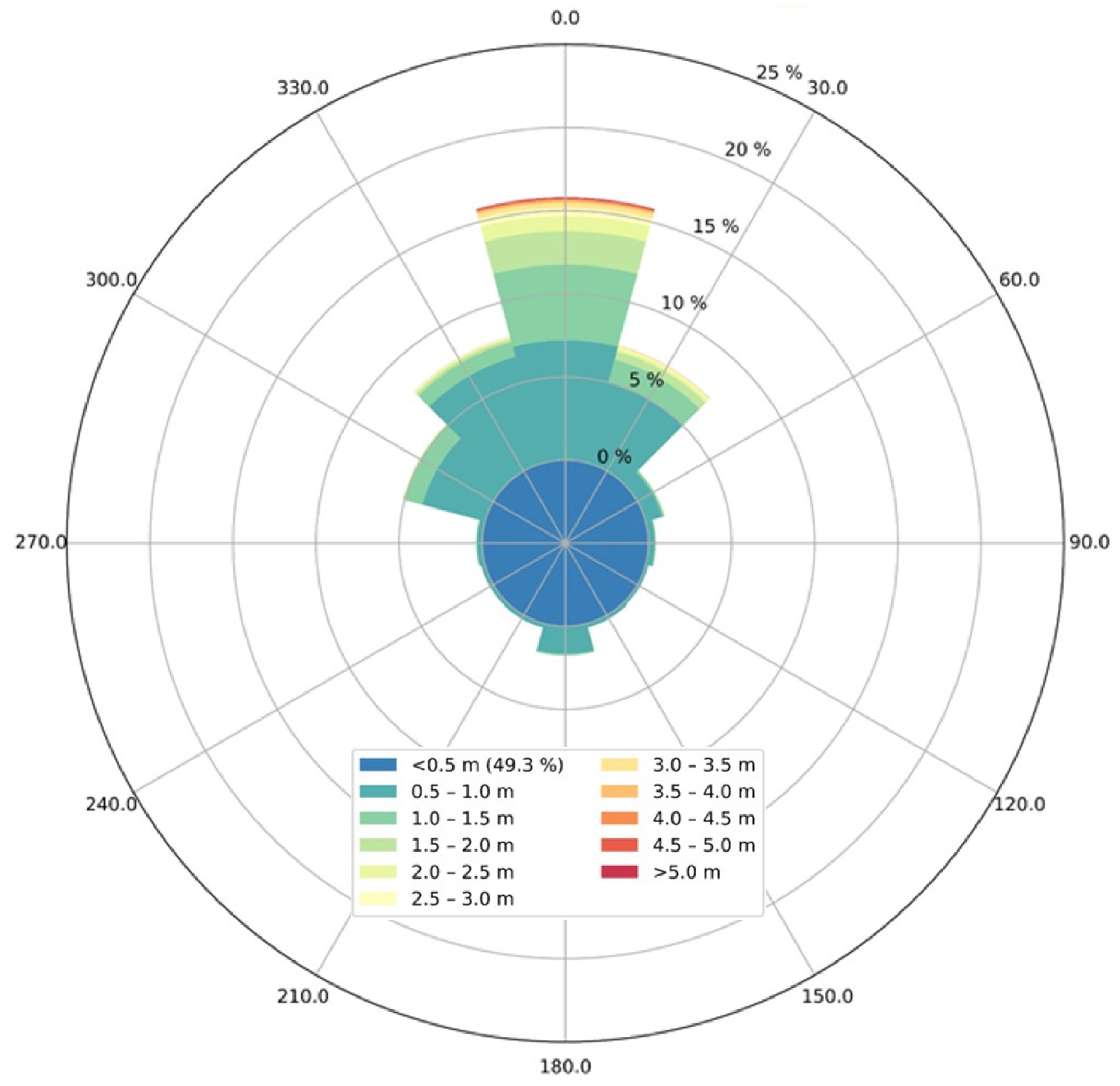
At this point, it should be noted that in order to provide a more realistic aspect to the idealized test case, it was selected to proceed with a non-artificial wave climate obtained from the Copernicus Marine Environment Monitoring Service [43]. Specifically, offshore sea-state wave characteristics ( H mo ,   T p ,   MWD ) at hourly intervals were obtained from the regional package entitled MEDSEA_MULTIYEAR_WAV [44], for a period spanning from 1993 to 2019. This data package was produced by the Mediterranean Sea Waves forecasting system, which encompasses a wave model based on the WAM Cycle 4.5.4. From this data package, wave characteristics were extracted at a position located 40.469° N, 19.3940° E. Wave data were classified into equally spaced groups of wave heights at intervals of 0.50 m for each mean wave direction and the MWD was broken down into bins at 22.5° intervals, i.e., 16 sectors (N, NNE, NE, ENE, E, ESE, SE, SSE, S, SSW, SW, WSW, W, WNW, NW, and NNW). A wave rose plot of the obtained wave climate is illustrated in Figure 2. The radial length of each bin in the rose plot represents the frequency, whereas the distribution of colors on each bar represents the wave height groups according to the legend.
It can be deduced that given the orientation of the coastline and the obtained wave climate shown in Figure 2, seven dominant wave directions can be considered vital in inducing the morphological changes at the study area, namely SSW, SW, WSW, W, WNW, NW, and NNW. Additionally, the wave climate can be considered relatively mild with 68% of sea-states having a significant wave height H s < 0.5   m .
Three forcing simulation sets have been conducted in order to intercompare results and investigate whether the presented methodology can lead to a considerable reduction of computational effort without compromising the reliability of the morphological model results. Therefore, the following tests were set up:
  • A “brute force” simulation set (BF) containing a detailed representation of the wave climate composed of 36 sea-states propagating from the dominant wave directions.
  • A simulation set with the elimination of sea-states considered unable to initiate sediment motion by implementing the developed ANN to reduce the input dataset. Thereafter seven “annual equivalent” wave representatives are obtained from the reduced dataset, one for each dominant wave direction and are used to force the integrated models. This simulation will be thereafter denoted as “EW w/ANN”
  • A simulation set with the forcing conditions being the seven “annual equivalent” wave representatives considering the full wave climate. This simulation will be thereafter denoted as “EW”
To evaluate the performance of the morphological model the commonly used assessment metric entitled Brier Skill Score (BSS) [45] was calculated through the following relationship:
BSS = 1 MSE ( Y , X ) MSE ( B , X )
where: Y denotes the modelled quantity, X denotes measurements, and B denotes a baseline prediction. Table 3 shows the classification scores for the BSS according to [44] in order to evaluate the performance of a specific morphological evolution model.
For the particular case, considering the lack of available measurements, the quantity X is considered to be the results of bed level change rates obtained by the “benchmark” BF simulation, whereas Y is the corresponding results obtained from simulation sets “EW w/ANN” and “EW” respectively. As a baseline prediction, an undisturbed bed assuming zero bed level change rates was considered. The BSS were calculated considering an extend of ± 67.5 ° from each breakwater tip, to replicate the shadow area of the structure. The evaluation area as well as an overview of the bathymetry for the bed slope of 1:50 is showcased in Figure 3.

3.2. Real-Field Test Case

The proposed methodological framework has also been implemented in a real-field case study in order to assess model performance and reliability of results in a more complex bathymetric domain and coastline shape. The study area is located in Rethymno on the Island of Crete, Greece, in the Eastern Mediterranean Sea. The population of Rethymno city stands at 32,468 inhabitants, rendering it the third most populous urban area in Crete. The city is the center of commercial, administrative, and cultural activities and many human activities are concentrated in the vicinity of the port area. The area of interest encompasses the aforementioned port infrastructure and an adjacent coastline at the east of the port, approximately 4 km long. The particular study area has been at the forefront of research efforts by the authors of this work, with regard to the evaluation of annual morphological bed evolution [14] and hazards due to impending coastal flooding [46,47].
The bed at the coastal zone is mildly sloping and is composed mostly of sand material of fine grading. Hence, a bed slope ( tan β ) (estimated by taking advantage of bathymetric data from nautical maps of the Navionics [48] database) of 1:50 was considered along with a median sediment diameter d 50   = 0.15 mm. These values are provided as a prerequisite to the ANN for the estimation of the maximum bed shear stress.
Morphological modelling simulations were carried out by implementing sequentially the HMS model for wave propagation, HYD for the prescription of the flow field, and SDT for the induced rates of bed level change. The HMS model is a wave model based on the hyperbolic form of the mild slope wave equation [49] enhanced with non-linear dispersion characteristics [24]. The model can also treat the generation and propagation of irregular unidirectional and multidirectional waves by employing the single summation model of [50] to decompose the wave spectrum. HMS was selected over PMS due to the presence of the port since the dominant processes of wave reflection and diffraction cannot be treated by the parabolic approximation of the mild slope equation. A total run time of 800 s and 1000 s was set for the HMS and HYD models respectively to ensure convergence of the solution, with a time step of 0.025 s and 0.05 s both satisfying the CFL condition.
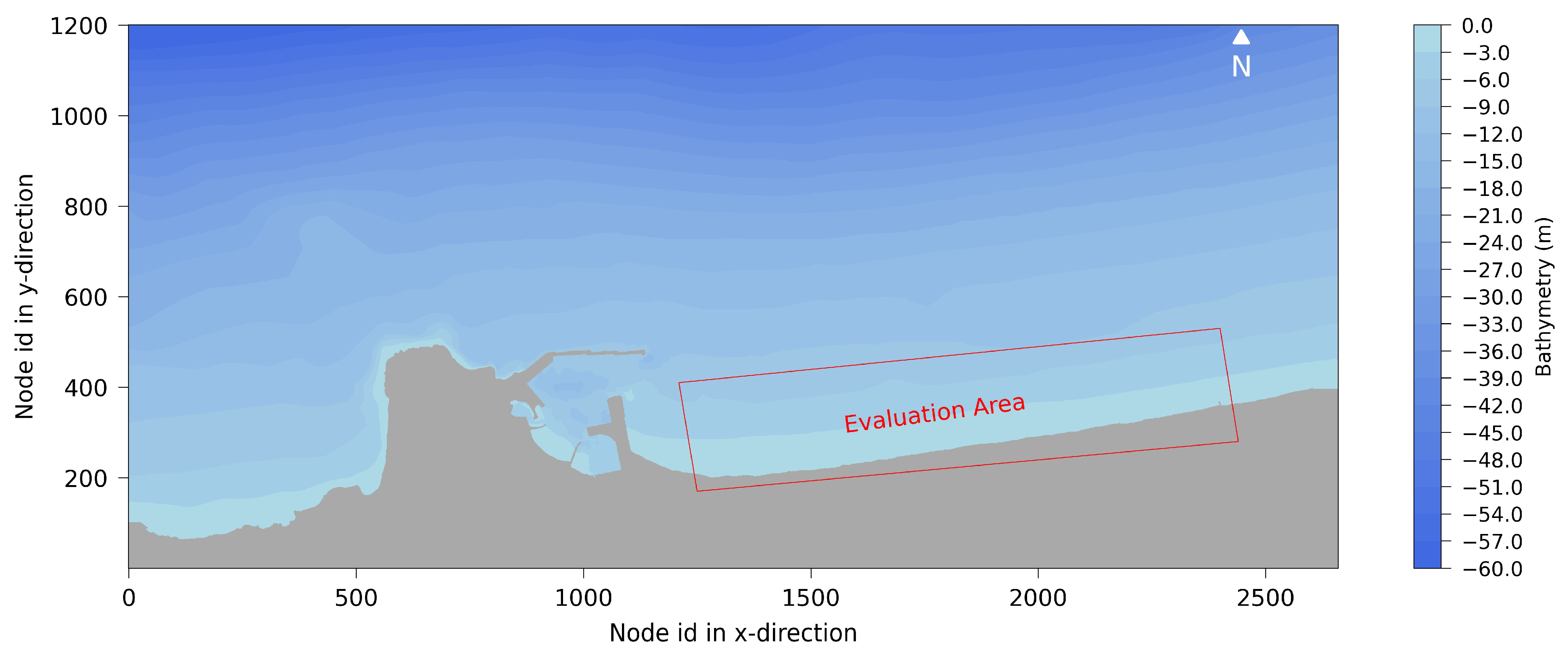
The bathymetry was resolved with a total number of 2660 cells in the x and 1200 cells in the y direction respectively. A constant grid size of 2.5 m was considered in both directions. The bathymetry of the study area, as inserted in the numerical models is showcased in Figure 4.
Similarly, to the idealized test case, offshore sea-state wave characteristics at hourly intervals were extracted from the regional MEDSEA_MULTIYEAR_WAV [44] package, for a period spanning from 1993 to 2019 at a location of 35.399849° N, 24.478480° E. Once again, the wave climate was divided into equally spaced groups of wave heights, with a step of 0.50 m for each mean wave direction bin and consequently, MWD bins were broken down into 22.5° intervals. A schematic overview of the annual wave climate offshore the study area is showcased in Figure 5.
From the above rose diagram, it can be deduced that the waves arriving from the north sector have the highest energy capacity since they are associated with the highest observed values of significant wave height along with the highest frequencies of occurrence f . The maximum value of H s encountered in the dataset is 6.37 m with a peak wave period T p   = 10.15 s and MWD   = 351.39°. Given the orientation of the shoreline, which is almost perpendicular to the northern sector, waves propagating from WNW, NW, NNW, N, NNE, NE, and ENE sectors are considered to contribute to the sediment transport regime and induce morphological changes.
The same procedure as the idealized case is herein followed to evaluate the morphological model results by conducting three sets of simulations:
  • A “brute force” simulation set (BF) containing a robust representation of the wave climate composed of 78 sea-states.
  • A simulation set with the elimination of sea-states considered unable to initiate sediment motion by implementing the developed ANN to reduce the input dataset. This simulation set will be thereafter denoted as “EW w/ANN” and contains a representative sea-state for each dominant wave direction.
  • A simulation set with the forcing conditions being the seven “annual equivalent” wave representatives after the elimination of wave records by employing an arbitrary threshold of H s < 0.5. This simulation will be thereafter denoted as “EW w/threshold”.
For the third simulation set it was selected to proceed with an approach followed by numerous research efforts [7,8], i.e., the elimination of wave records if their respective significant wave height does not exceed a certain threshold. The comparison between “EW w/ANN” and “EW w/threshold” simulation sets can provide a comprehensive evaluation of the performance of the methodology developed in the scope of this research and a cruder approach to eliminating lowly energetic sea-states based only on their significant wave height.
Evaluation of model results will be carried out in an area enclosed within the polygon shown in Figure 4, about 3.5 km long and reaching a depth of about 8 m and following the corresponding contour line. Once again, in the absence of measurements of bed elevation, the detailed BF simulation is considered a benchmark for the numerical model predictions.

4. Results and Discussion

In this section, the results obtained by performing the morphological modelling simulations will be presented and analyzed for the idealized test case, as well as the field case implementation.

4.1. Idealized Test Case

4.1.1. Obtained Representative Wave Conditions

A schematic overview of the retained and eliminated wave characteristics that are considered unable to initiate the sediment motion after implementing the ANN is showcased in Figure 6 for the bed slope of 1:50 and considering two characteristic grain sizes, namely d 50 = 1   mm and d 50 = 2   mm . In the same Figure the obtained representative wave conditions obtained for the respective simulation sets “EW w/ANN” and “EW” can also be observed. Considering the case of d 50 = 1   mm out of 236,664 wave records, implementation of the ANN lead to the elimination of 198,338 sea-states reducing the length of the dataset by about 84%. Similarly, considering a d 50 = 2 mm lead to the elimination of 221,425 sea-states and an effective reduction of the dataset to about 93%.
As expected, more sea-states are eliminated by increasing the median sediment diameter since larger bed shear stress is required to set the sediment grains into motion. In particular, the minimum H s considered to set the sediment into motion is 0.57 m for the case of d 50 = 1 mm, whereas a minimum value of H s = 0.82 m is required to entrain the sand of d 50 = 2 mm. However, these limits are not strict since the ANN predicts the values of bed shear stress based on the corresponding wave period, wave incidence angle, and bed slope. It is important to note that in the examined wave climate, due to the prevalence of “lowly” energetic sea-states, the representatives obtained from Equations (12) and (13) fall below the threshold set by the ANN, indicating that without the implementation of a threshold the influence of said sea-states may be overly estimated. The obtained representative sea-states along with the corresponding frequencies of occurrence for the simulation sets considering d 50 = 2 mm and tan β = 1:50, are showcased in Table 4.
As can be seen in Table 4, the sheer reduction of the dataset due to the elimination ordered by the ANN shifts the values of H e and T e to significantly more energetic pairs and drastically alters the frequency of occurrence of said events. Considering that all records that are eliminated from the dataset are considered to induce insignificant morphological changes and hence are considered “calm”, the frequencies of the representatives of “EW w/ANN” are rescaled to reflect this issue. Consequently, the total frequency of the “calm” conditions increases, whereas the representative waves have a smaller frequency of occurrence since, fewer wave records are considered able to initiate sediment motion.

4.1.2. Morphological Modelling Results and Evaluation

In this subsection, the results of the rate of bed level change predicted by the proposed methodology will be presented and evaluated.
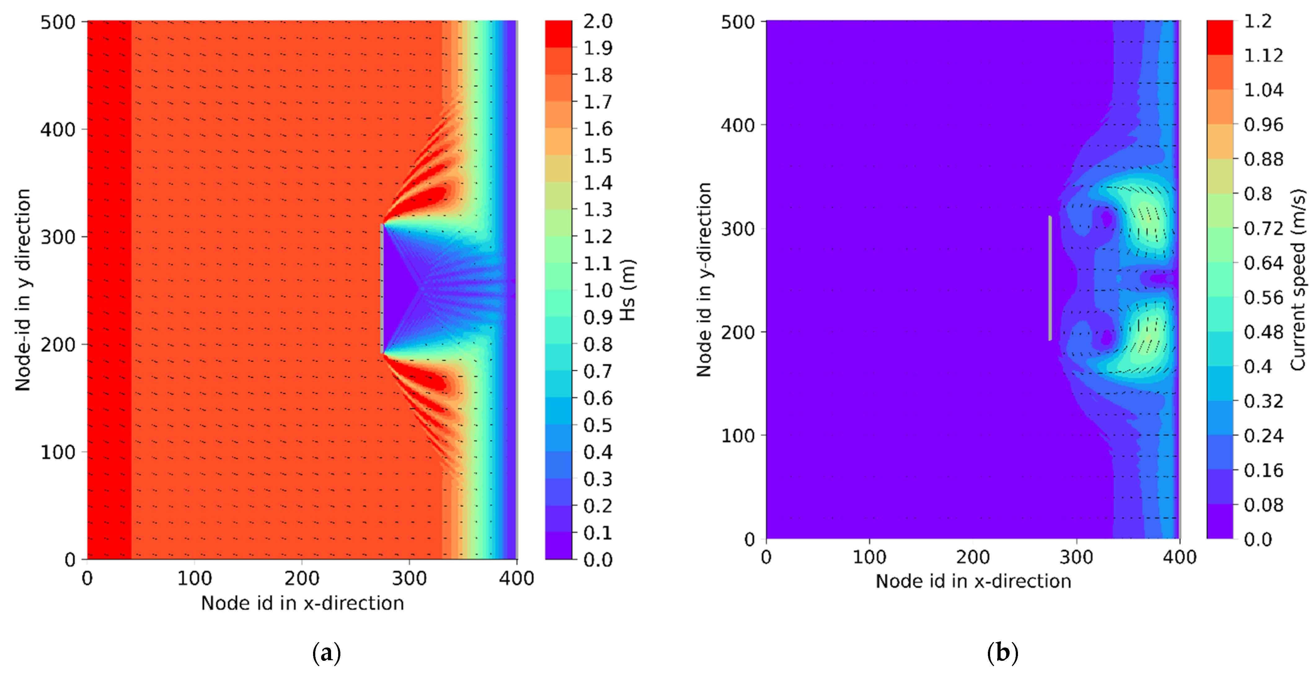
To provide insight into the obtained wave and hydrodynamic field simulated by the PMS and HYD models respectively, Figure 7 presents maps of the spatial distribution of the significant wave height and the current velocity considering a uni-directional wave with H s   = 2.0 m, T p   = 6.5 s, and MWD   = 270°.
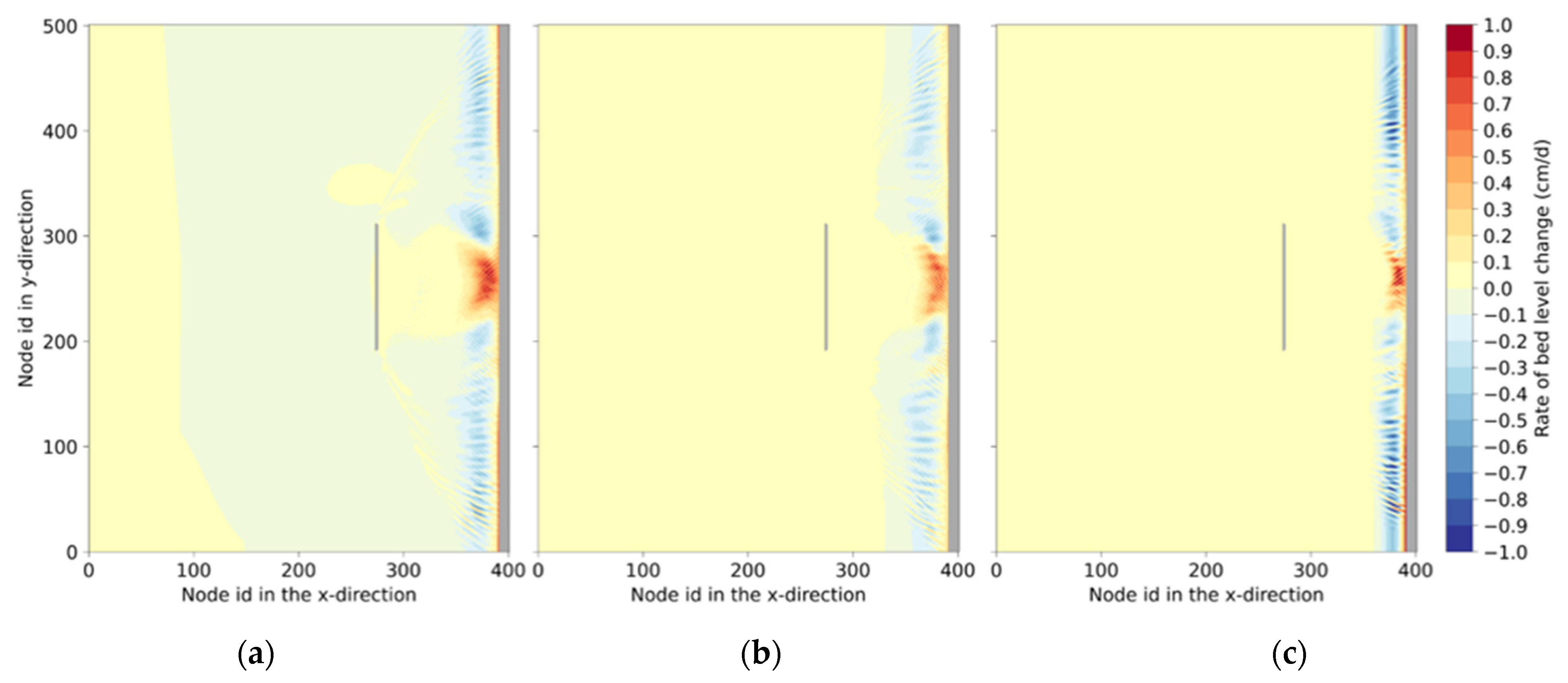
Thereafter, the integrated rate of bed level change obtained by the SDT model for the “BF”, “EW w/ANN”, and “EW” simulation sets are presented in Figure 8 for the case of d 50   = 1 mm and a tan β of 1:50. To obtain the integrated rates, each individual event is multiplied by its frequency of occurrence f and then they are all summed together resulting in an annual integrated rate of erosion/accretion over the whole computational grid.
From the visual inspection of the results, it can be deduced that in general the morphological response of both “EW w/ANN” and “EW” simulation sets can adequately reproduce the one obtained by the “BF” benchmark simulation set. However, observing the patterns of accretion and erosion more closely, it can be seen that the EW simulation underpredicts the extent of the accretive patterns at the lee of the breakwater while also overpredicting the intensity of the erosion rates outside the shadow area of the structure. Conversely, the obtained rates of bed level change predicted by the “EW w/ANN” simulations are almost identical to the benchmark simulation as far as the extent of the obtained patterns, with a rather inconsequential underprediction of the intensity of the erosion/accretion rates.
In Table 5, the calculated BSS for the sensitivity tests IC1 through IC6 (the parametrizations of these tests were previously shown in Table 2) are compiled and shown for both simulation sets of the proposed methodology and the classical approach.
As can be seen on Table 5, the calculated BSS values obtained by implementing the presented methodology are classified as “Excellent” for all “EW/w ANN” test simulations, with regards to the classification of [45]. The highest skill scores are obtained when dealing with smaller grain sizes and a small deterioration is observed with the highest grain size of d 50   = 2 mm. This can in part be attributed to the fact that since the values of the critical shear stress increase as the sediment grain diameter increases, some sea-states are eliminated but, in turn, might produce some rates of bed level change in shallower water depths. The BSS and performance of the model do not exhibit a particular trend for the steeper bed slope of 1:20.
On the contrary, the classical “EW” approach of performing the same simulations calculating an annual “equivalent” set of wave characteristics from the full set of wave records produces significantly worse results. In particular, only test IC1 is classified as “Excellent” with respect to the BSS classification, with test IC6 indicating a poor model performance. The intermediate tests are classified as either Fair or Good. The worse performance of the classical approach for this case can be attributed to the over-estimation of the contribution of lowly energetic sea-states in the dataset which are associated with high frequencies of occurrence and significantly influence the obtained morphological model results. Consequently, the idealized test case and the corresponding sensitivity analysis validate the utilization of the proposed methodology incorporating the ANN since it achieves both a reduction of computational effort and enhances the accuracy of the model predictions.

4.2. Real-Field Case Study

In this section, the results obtained by the set of simulations carried out for the study area of Rethymno, Crete, Greece will be presented. This case study is of particular importance since it will showcase the performance of the proposed methodology in a more complex case and with the use of a different wave model (HMS) than the one utilized to train the ANN.

4.2.1. Obtained Representative Wave Conditions

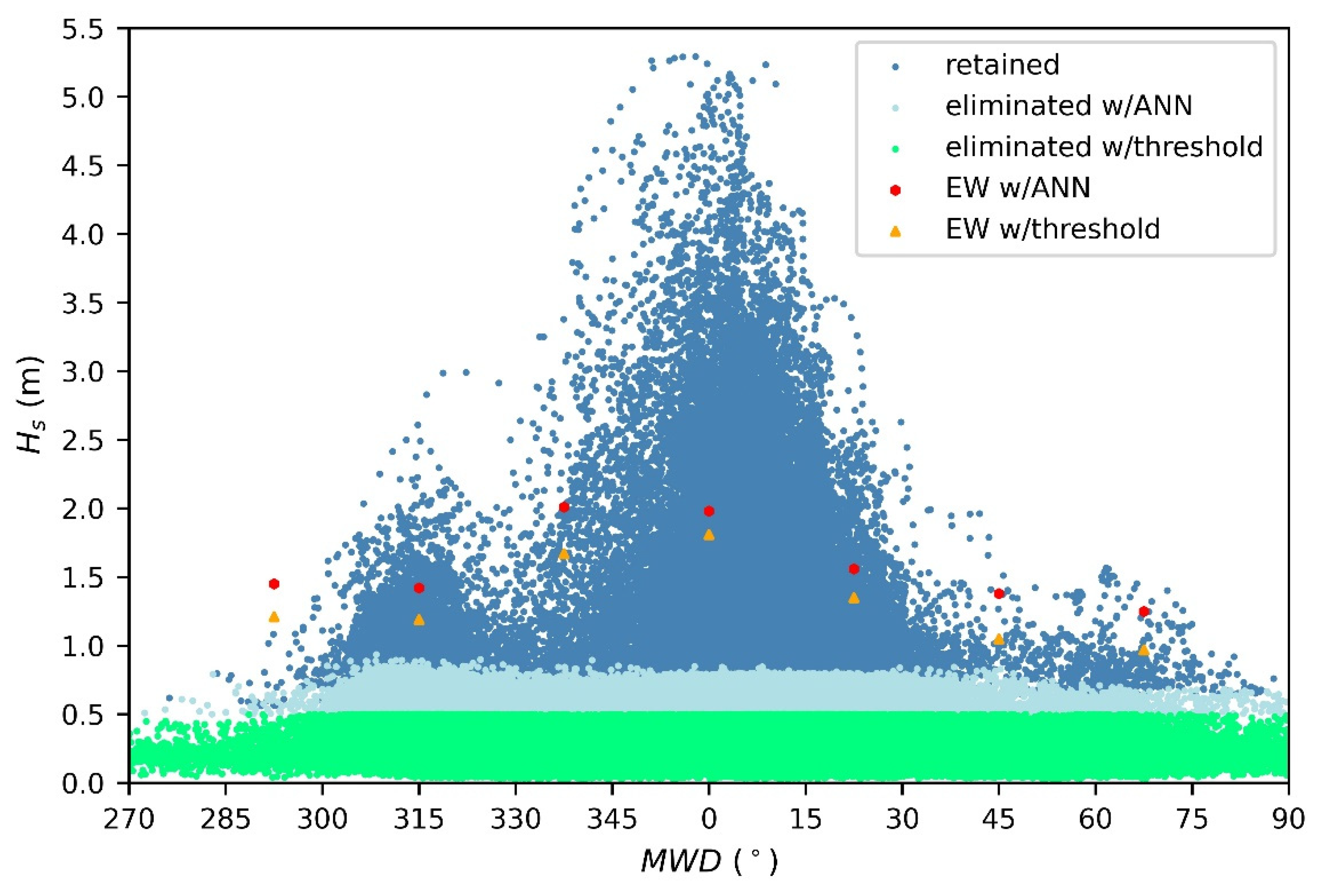
The sea-states were eliminated by implementing the ANN as well as through an arbitrary threshold of H s   = 0.5 m are showcased in Figure 9, for the dataset covering an extent of 1993–2019. Out of the total of 236,664 wave records, the proposed methodology led to the elimination of 173,792 sea-states while the corresponding number is 131,456 by employing the arbitrary threshold.
As shown in Figure 9, more sea-states are considered unable to initiate sediment motion and are hence eliminated from the dataset by employing the proposed methodology incorporating the ANN. It is notable that although a minimum of H s   = 0.55 m was retained in the “EW w/ANN” simulation sets, this sea-state is associated with a peak wave period of T p   = 12.28 s indicating that long waves are more capable of initiating sediment motion due to a wider surf zone. Employing the arbitrary threshold pushes the representatives of the “EW w/threshold” simulation set closer to the respective ones of “EW w/ANN” however due to the difference in the length of the corresponding reduced datasets, the wave representatives have different frequencies of occurrence. In the directional bins where more energetic sea-states are present in the dataset (i.e., waves propagating from the N sector) the representative characteristics are even more similar in values.

4.2.2. Morphological Modelling Results and Evaluation

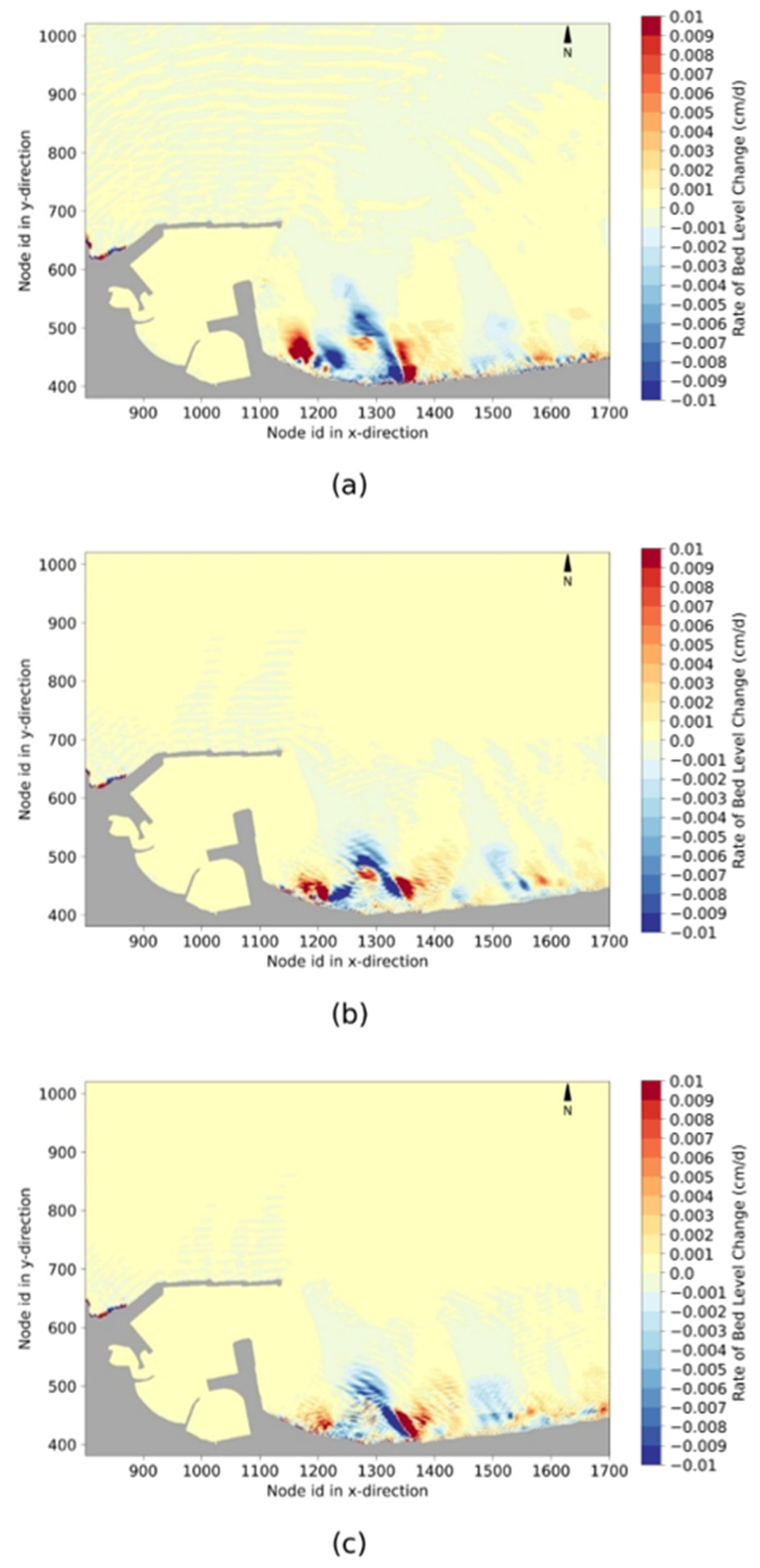
After executing in sequence the HMS, HYD, and SDT models for each sea-state of the three distinct simulation sets, an integrated initial rate of bed level change was obtained for the “BF”, “EW w/ANN”, and “EW w/threshold” respectively and the results are shown in Figure 10.
Both simulations are deemed as “Good” with regards to the BSS classification, however, an improvement on the obtained BSS is obtained when implementing the filtering criterion as presented in the framework of the proposed methodology. The score is deemed acceptable for practical applications, especially considering that lower BSS values are expected when the magnitude of the changes is rather small [45]. It is noteworthy that even though the obtained representative wave conditions of “EW w/ANN” and “EW w/threshold” are quite similar in values, the interplay between all the physical processes considered when training the ANN leads to an improvement of the predictions of the rates of bed level change. Expanding on this, the effect of the wave period and median sediment diameter significantly affect the obtained values of the bed shear stress and should be considered when desiring to discard lowly energetic sea-states from a dataset of offshore sea-state wave characteristics. Furthermore, it is considered that the proposed methodology incorporating an ANN produced satisfactory predictions of the rate of bed level change due to the combined effect of waves and currents for a complex case, especially when considering that different phase-resolving wave models were used to train the ANN and perform the simulations for the real-field case study.

5. Conclusions

In the present paper, a methodological framework aiming to enhance morphological bed evolution predictions by eliminating sea-states considered unable to initiate sediment motion by combining numerical modelling and an Artificial Neural Network (ANN) was presented. The methodology considers a variety of parameters influencing the prediction of the bed shear-stress, the factor responsible for setting sediments into motion, such as the offshore wave characteristics, bed slope, and median sediment diameter. Several simulations with a wave and hydrodynamic model were used to train an ANN in order to facilitate the accurate and fast elimination of sea-states that have little to no effect on the sediment transport regime.
The proposed methodology was firstly implemented in an idealized case study of an alongshore uniform beach protected by a detached breakwater. Six distinct sensitivity tests were performed to assess the performance of the methodology. Two simulation sets were compared: firstly, the estimation of the rates of bed level change by calculating annual “equivalent” wave characteristics after the elimination of sea-states as ordered by the ANN, and secondly, by considering the full dataset. The proposed methodology resulted in a significant improvement in the obtained BSS values, which were all classified as “Excellent” compared to the more classical approach which showed significantly worse performance.
The methodology was applied in a real-field study area in Rethymno, Crete, Greece, and the results were compared to a simulation considering a crude elimination of wave records with a significant wave height lower than 0.5 m. Once again predictions of the rates of bed level change were marginally improved by implementing the proposed methodology, signifying the importance of considering the interplay of the characteristics and processes influencing the bed-shear stress under combined waves and currents.
Therefore, it is considered that the proposed methodology will be a valuable tool for coastal engineers and scientists, desiring to enhance the reliability of morphological bed evolution predictions by minimizing the computational burden. The training and implementation of an ANN in the methodological framework further exemplifies the aspect of computational efficiency since the decision on which sea-states to be eliminated is achieved in only a few seconds.

Author Contributions

Conceptualization, A.P., M.C. and A.M.; methodology, A.P., M.C. and A.M.; software, A.P., M.C. and A.M.; validation, A.P., M.C. and A.M.; formal analysis, A.P., M.C., A.M. and V.T.; investigation, A.P., M.C., A.M. and V.T.; resources, M.C., A.M. and V.T.; data curation, A.P., M.C. and A.M.; writing—original draft preparation, A.P. and M.C.; writing—review and editing, A.M. and V.T.; visualization, A.P. and A.M.; supervision, M.C., A.M. and V.T.; project administration, M.C. and A.M.; funding acquisition, M.C. and A.M. All authors have read and agreed to the published version of the manuscript.

Funding

This research has been co-financed by the European Regional Development Fund of the European Union and Greek national funds through the Operational Program Competitiveness, Entrepreneurship and Innovation, under the call RESEARCH–CREATE–INNOVATE (project code: T2EDK-03811).

Institutional Review Board Statement

Not applicable.

Informed Consent Statement

Not applicable.

Conflicts of Interest

The authors declare no conflict of interest.

References

  1. Roelvink, D.; Reniers, A. A Guide to Modeling Coastal Morphology, 1st ed.; Word Scientific: Singapore, 2012; p. 292. [Google Scholar]
  2. de Vriend, H.J.; Zyserman, J.; Nicholson, J.; Roelvink, J.A.; Péchon, P.; Southgate, H.N. Medium-term 2DH coastal area modelling. Coast. Eng. 1993, 21, 193–224. [Google Scholar] [CrossRef] [Green Version]
  3. Roelvink, J.A. Coastal Morphodynamic Evolution Techniques. Coast. Eng. 2006, 53, 277–287. [Google Scholar] [CrossRef]
  4. Lesser, G.R. An Approach to Medium-Term Coastal Morphological Modelling. Ph.D. Thesis, Delft University of Technology, Delft, The Netherlands, 4 June 2009. [Google Scholar]
  5. Borah, D.K.; Balloffet, A. Beach Evolution Caused by Littoral Drift Barrier. J. Waterw. Port Coast. Ocean Eng. 1985, 111, 645–660. [Google Scholar] [CrossRef]
  6. Brown, J.M.; Davies, A.G. Methods for Medium-Term Prediction of the Net Sediment Transport by Waves and Currents in Complex Coastal Regions. Cont. Shelf Res. 2009, 29, 1502–1514. [Google Scholar] [CrossRef]
  7. Walstra, D.J.R.; Hoekstra, R.; Tonnon, P.K.; Ruessink, B.G. Input Reduction for Long-Term Morphodynamic Simulations in Wave-Dominated Coastal Settings. Coast. Eng. 2013, 77, 57–70. [Google Scholar] [CrossRef]
  8. Benedet, L.; Dobrochinski, J.P.F.; Walstra, D.J.R.; Klein, A.H.F.; Ranasinghe, R. A morphological modeling study to compare different methods of wave climate schematization and evaluate strategies to reduce erosion losses from a beach nourishment project. Coast. Eng. 2016, 112, 69–86. [Google Scholar] [CrossRef]
  9. de Queiroz, B.; Scheel, F.; Caires, S.; Walstra, D.J.; Olij, D.; Yoo, J.; Reniers, A.; de Boer, W. Performance Evaluation of Wave Input Reduction Techniques for Modeling Inter-Annual Sandbar Dynamics. J. Mar. Sci. Eng. 2019, 7, 148. [Google Scholar] [CrossRef] [Green Version]
  10. Chonwattana, S.; Weesakul, S.; Vongvisessomjai, S. 3D Modeling of Morphological Changes Using Representative Waves. Coast. Eng. J. 2005, 47, 205–229. [Google Scholar] [CrossRef]
  11. Karambas, T.V.; Koutandos, E.V.; Kampanis, N.A. Numerical Simulation of Wave-Induced Morphology Evolution. Marit. Eng. 2013, 166, 113–124. [Google Scholar] [CrossRef]
  12. Papadimitriou, A.; Tsoukala, V. Performance Evaluation of the K-Means Clustering Algorithm for the Prediction of Annual Bed Morphological Evolution. In Proceedings of the 7th IAHR Europe Congress, Athens, Greece, 7–9 September 2022; pp. 161–162. [Google Scholar]
  13. Pletcha, S.; Sancho, F.; Silva, P.; Dias, J.M. Representative Waves for Morphological Simulations. J. Coast. Res. 2007, SI 50, 995–999. [Google Scholar]
  14. Papadimitriou, A.; Panagopoulos, L.; Chondros, M.; Tsoukala, V. A Wave Input-Reduction Method Incorporating Initiation of Sediment Motion. J. Mar. Sci. Eng. 2020, 8, 597. [Google Scholar] [CrossRef]
  15. Bosboom, J.; Stive, M.J.F. Coastal Dynamics; TU Delft Open Textbooks: Delft, The Netherlands, 2022; p. 579. [Google Scholar]
  16. Soulsby, R.L. Dynamics of Marine Sands: A Manual for Practical Applications, 1st ed.; Thomas Telford: London, UK, 1997; p. 249. [Google Scholar]
  17. Shields, I.A. Application of Similarity Principles and Turbulence Research to Bed-Load Movement; U.S. Soil Conservation Service Cooperative Laboratory; Ott, W.P.; van Uchelen, J.C., Translators; Hydrodynamics Laboratory Publication, California Institute of Technology: Pasadena, CA, USA, 1936; Volume 167. [Google Scholar]
  18. Grant, W.D.; Madsen, O.S. Combined Wave and Current Interaction with a Rough Bottom. J. Geophys. Res. Ocean. 1979, 84, 1797–1808. [Google Scholar] [CrossRef]
  19. Fredsøe, J. Turbulent Boundary Layer in Wavecurrent Motion. J. Hydraul. Eng. 1984, 110, 1103–1120. [Google Scholar] [CrossRef]
  20. Davies, A.G.; Soulsby, R.L.; King, H.L. A Numerical Model of the Combined Wave and Current Bottom Boundary Layer. J. Geophys. Res. Ocean. 1988, 93, 491–508. [Google Scholar] [CrossRef]
  21. Soulsby, R.L.; Hamm, L.; Klopman, G.; Myrhaug, D.; Simons, R.R.; Thomas, G.P. Wave-Current Interaction within and Outside the Bottom Boundary Layer. Coast. Eng. 1993, 21, 41–69. [Google Scholar] [CrossRef]
  22. Swart, D.H. Offshore Sediment Transport and Equilibrium Beach Profiles. Ph.D. Thesis, Delft University of Technology, Delft, The Netherlands, 18 December 1974. [Google Scholar]
  23. Soulsby, R.L.; Whitehouse, R.J. Threshold of sediment motion in coastal environments. In Proceedings of the 13th Australasian Coastal and Ocean Engineering Conference and the 6th Australasian Port and Harbour Conference, Canterbury, UK, 28–30 September 1997. [Google Scholar]
  24. Chondros, M.K.; Metallinos, A.S.; Memos, C.D.; Karambas, T.V.; Papadimitriou, A.G. Concerted Nonlinear Mild-Slope Wave Models for Enhanced Simulation of Coastal Processes. Appl. Math. Model. 2021, 91, 508–529. [Google Scholar] [CrossRef]
  25. Saltelli, A. Sensitivity Analysis for Importance Assessment. Risk Anal. 2002, 22, 579–590. [Google Scholar] [CrossRef] [PubMed]
  26. MacQueen, J. Some Methods for Classification and Analysis of Multivariate Observations. In Proceedings of the 5th Berkeley Symposium on Mathematical Statistics and Probability, Berkeley, CA, USA, 1 January 1967. [Google Scholar]
  27. Miche, M. Le Pouvoir Réfléchissant des Ouvrages Maritimes Exposés à l’action de La Houle; Technical Report; Annales de Ponts et Chaussées, École nationale des Ponts et Chaussées: Paris, France, 1951. [Google Scholar]
  28. Berkhoff, J.C.W. Computation of Combined Refraction-Diffraction. In Proceedings of the 13th International Conference on Coastal Engineering, Vancouver, BC, Canada, 10–14 July 1972. [Google Scholar]
  29. Kirby, J.T.; Dalrymple, R.A. A parabolic equation for the combined refraction diffraction of Stokes waves by mildly varying topography. J. Fluid Mech. 1983, 136, 453–466. [Google Scholar] [CrossRef] [Green Version]
  30. Kirby, J.T. Higher-Order Approximations in the Parabolic Equation Method for Water Waves. J. Geophys. Res. 1986, 91, 933–952. [Google Scholar] [CrossRef]
  31. Kirby, J.T. Rational approximations in the parabolic equation method for water waves. Coast. Eng. 1986, 10, 355–378. [Google Scholar] [CrossRef]
  32. Battjes, J.A.; Janssen, J.P.F.M. Energy Loss and Set-Up Due To Breaking of Random Waves. In Proceedings of the Coastal Engineering Conference, Hamburg, Germany, 27 August–3 September 1979. [Google Scholar]
  33. Putnam, J.A.; Johson, J.W. The dissipation of wave energy by bottom friction. Eos Trans. Am. Geophys. Union 1949, 30, 67–74. [Google Scholar] [CrossRef]
  34. Kirby, J.T.; Dalrymple, R.A. An approximate model for nonlinear dispersion in monochromatic wave propagation models. Coast. Eng. 1986, 9, 545–561. [Google Scholar] [CrossRef]
  35. Xia, M.; Mao, M.; Niu, Q. Implementation and comparison of the recent three-dimensional radiation stress theory and vortex-force formalism in an unstructured-grid coastal circulation model. Estuar. Coast. Shelf Sci. 2020, 240, 106771. [Google Scholar] [CrossRef]
  36. Moghimi, S.; Klingbeil, K.; Gräwe, U.; Burchard, H. A direct comparison of a depth-dependent Radiation stress formulation and a Vortex force formulation with a three-dimensional coastal ocean model. Ocean Model. 2013, 70, 132–144. [Google Scholar] [CrossRef]
  37. Van Rijn, L.C. Unified View of Sediment Transport by Currents and Waves. I: Initiation of Motion, Bed Roughness, and Bed-Load Transport. J. Hydraul. Eng. 2007, 133, 649–667. [Google Scholar] [CrossRef] [Green Version]
  38. van Rijn, L.C. Unified View of Sediment Transport by Currents and Waves. II: Suspended Transport. J. Hydraul. Eng. 2007, 133, 668–689. [Google Scholar] [CrossRef]
  39. Niu, Q.; Xia, M.; Ludsin, S.; Chu, P.; Mason, D.; Rutherford, E. High-turbidity events in Western Lake Erie during ice-free cycles: Contributions of river-loaded vs. resuspended sediments. Limnol. Oceanogr. 2018, 63, 2545–2562. [Google Scholar] [CrossRef] [Green Version]
  40. Chou, Y.-J.; Nelson, K.; Holleman, R.; Fringer, O.; Stacey, M.; Lacy, J.; Monismith, S.; Koseff, J. Three-Dimensional Modeling of Fine Sediment Transport by Waves and Currents in a Shallow Estuary. J. Geophys. Res. Ocean. 2018, 123, 4177–4199. [Google Scholar] [CrossRef] [Green Version]
  41. Long, W.; Kirby, J.T.; Shao, Z. A Numerical Scheme for Morphological Bed Level Calculations. Coast. Eng. 2008, 55, 167–180. [Google Scholar] [CrossRef]
  42. Keras: The Python Deep Learning API. Available online: https://keras.io/ (accessed on 18 September 2022).
  43. Coppernicus Marine Environment Monitoring Service CMEMS. Available online: http://marine.copernicus.eu/ (accessed on 18 September 2022).
  44. Korres, G.; Ravdas, M.; Zacharioudaki, A. [Dataset] Mediterranean Sea Waves Hindcast (CMEMS MED-Waves). Available online: https://resources.marine.copernicus.eu/?option=com_csw&view=details&product_id=MEDSEA_MULTIYEAR_WAV_006_012 (accessed on 18 September 2022).
  45. Sutherland, J.; Peet, A.H.; Soulsby, R.L. Evaluating the performance of morphological models. Coast. Eng. 2004, 51, 917–939. [Google Scholar] [CrossRef]
  46. Tsoukala, V.K.; Chondros, M.; Kapelonis, Z.G.; Martzikos, N.; Lykou, A.; Belibassakis, K.; Makropoulos, C. An Integrated Wave Modelling Framework for Extreme and Rare Events for Climate Change in Coastal Areas—The Case of Rethymno, Crete. Oceanologia 2016, 58, 71–89. [Google Scholar] [CrossRef]
  47. Chondros, M.; Tsoukala, V.; Metallinos, A.; Papadimitriou, A.; Memos, C. A Coastal Flood Early-Warning System Based on Offshore Sea State Forecasts and Artificial Neural Networks. J. Mar. Sci. Eng. 2021, 9, 1272. [Google Scholar] [CrossRef]
  48. NAVIONICS: A Garmin Company. Available online: https://webapp.navionics.com/ (accessed on 11 September 2022).
  49. Copeland, G.J.M. A Practical Alternative to the “Mild-Slope” Wave Equation. Coast. Eng. 1985, 9, 125–149. [Google Scholar] [CrossRef]
  50. Yu, Y.X.; Liu, S.X.; Li, L. Numerical simulation of multi-directional waves. In Proceedings of the International Society of Offshore and Polar Engineers Conference, Edinburgh, UK, 11–16 August 1991. [Google Scholar]
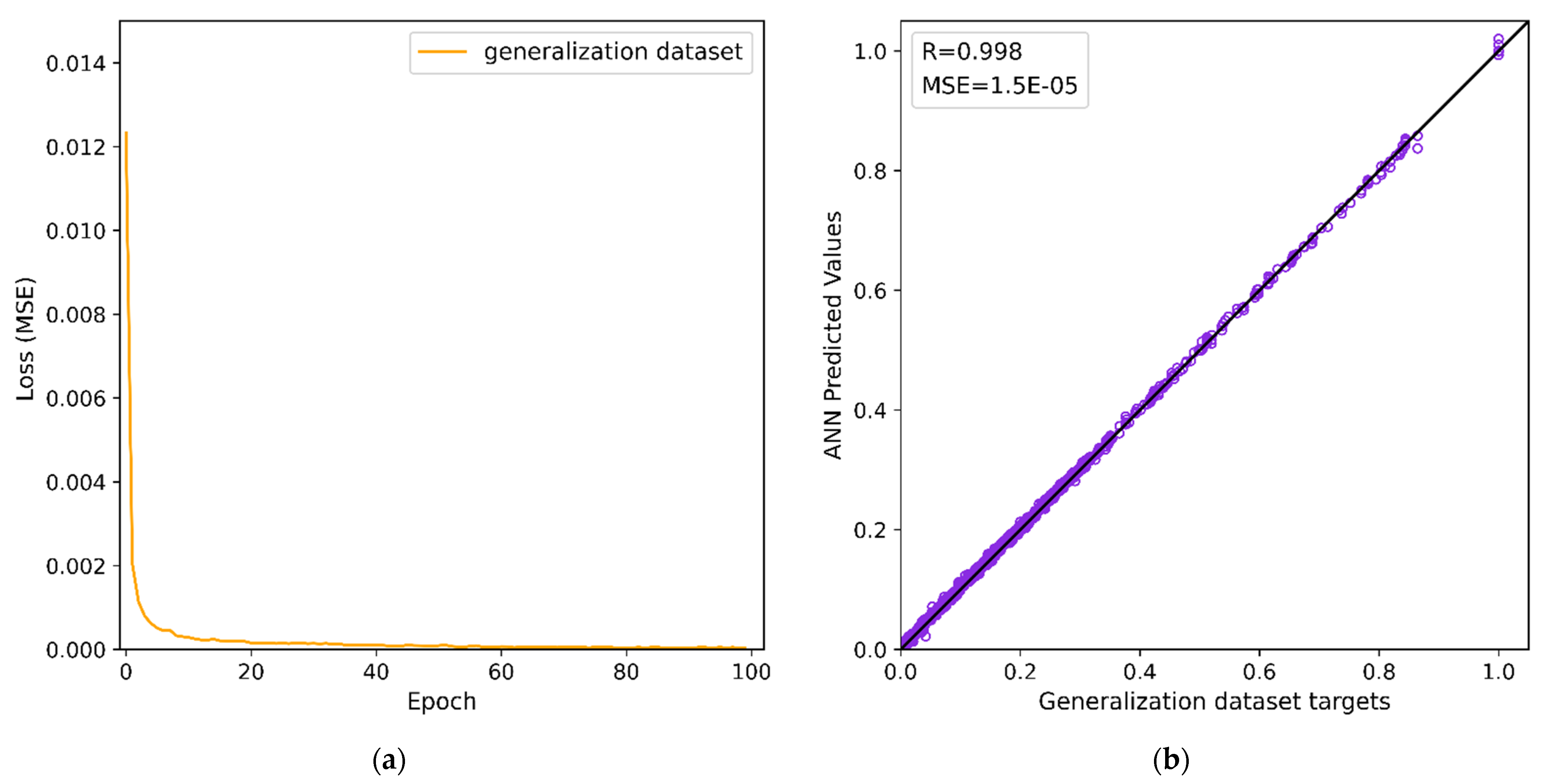
Figure 1. Error and performance metrics of the training procedure: (a) Evolution of the MSE during the training and validation of the generalization dataset (b) ANN predicted values against the respective targets of the generalization dataset.
Jmse 10 01621 g001
Figure 2. Wave rose plot of the mean annual wave climate for the idealized test case.
Jmse 10 01621 g002
Figure 3. Selected overview of the bathymetry of the idealized case, evaluation area of the BSS (enclosed in the red rectangle). The shadow area of the breakwater is denoted by the black lines.
Jmse 10 01621 g003
Figure 4. Bathymetry of the study area in Rethymno, Crete, Greece.
Jmse 10 01621 g004
Figure 5. Wave rose plot of the mean annual wave climate offshore the study area of Rethymno.
Jmse 10 01621 g005
Figure 6. Retained (blue markers) and eliminated (light blue markers) sea-states by implementing the proposed methodology for the idealized case of bed slope 1:50 for (a) d50 = 1 mm and (b) d50 = 2 mm. The red data points denote the representatives for the simulation EW w/ANN and the orange those by implementing EW in the full dataset.
Jmse 10 01621 g006
Figure 7. Spatial distribution of (a) significant wave height simulated with PMS and (b) hydrodynamic circulation simulated with HYD, for the idealized case with slope 1:50.
Jmse 10 01621 g007
Figure 8. Integrated annual rate of bed level change for the: (a) “BF” (b) “EW w/ANN”, and (c) “EW” simulation sets.
Jmse 10 01621 g008
Figure 9. Retained (blue markers) and eliminated (light blue markers) sea-states by implementing the proposed methodology and by employing an arbitrary threshold (green markers). The red data points denote the representatives for the simulation “EW w/ANN” and the orange those by following the “EW w/threshold” approach.
Jmse 10 01621 g009
Figure 10. Integrated annual rate of bed level change for the (a) “BF” (b) “EW w/ANN”, and (c) “EW w/threshold” simulation sets.
Jmse 10 01621 g010
Table 1. Lower and upper boundaries of the Input Parameters (IP) are considered.
H s   [ m ] T p   [ s ] a o   [ ° ] d 50   [ mm ] tan β   [ ]
minimum00−900.061:50
maximum715902.01:5
Table 2. Examined scenarios and combinations of the considered values of d 50 and tan β .
Test ID d 50   [ mm ] tan β
IC10.11:50
IC21.01:50
IC32.01:50
IC40.11:20
IC51.01:20
IC62.01:20
Table 3. Classification for the BSS (Adapted with permission from Ref [45], 2004, Elsevier).
BSS
Excellent (E)1.0–0.5
Good (G)0.5–0.2
Reasonable/Fair (R/F)0.2–0.1
Poor (P)0.1–0.0
Bad (B)<0.0
Table 4. Obtained representative sea-states by implementing the proposed methodology (EW w/ANN).
SectorEW w/ANNEW
He (m)Te (s)MWD (°)f (%)He (m)Te (s)MWD (°)f (%)
SSW0.967.94202.50.97650.626.04202.513.30
SW1.048.35225.01.65680.606.07225.020.46
WSW0.987.87247.50.27470.525.55247.55.78
W1.027.08270.00.24470.535.18270.05.93
WNW1.156.72292.52.52890.725.10292.527.86
NW0.996.75315.00.75420.514.58315.024.93
NNW0.817.36337.50.00340.465.89337.50.50
Table 5. Calculated BSS and classification of the “EW w/ANN” and “EW” simulation sets.
Test IDEW w/ANNEW
IC10.92 (E)0.65 (E)
IC20.77 (E)0.24 (G)
IC30.65 (E)0.22 (G)
IC40.86 (E)0.45 (G)
IC50.86 (E)0.19 (R/F)
IC60.72 (E)0.04 (P)
Publisher’s Note: MDPI stays neutral with regard to jurisdictional claims in published maps and institutional affiliations.