Kriging Model for Reliability Analysis of the Offshore Steel Trestle Subjected to Wave and Current Loads

Abstract

Offshore steel trestles (OSTs) are exposed to severe marine environments with stochastic wave and current loads, making structural safety assessment challenging and difficult. Reliability analysis is a suitable way to consider both wave and current loading intensity uncertainties, but the implicit and complex limit state functions of the reliability analysis usually imply huge computational costs. This paper proposes an efficient reliability analysis framework for OST using the kriging model of optimal linear unbiased estimation. The surrogate model is built with stochastic waves, current parameters, and the corresponding load factors. The framework is then used to evaluate the reliability of an example OST subjected to wave and current loads at three limit states of OST, including first yield (FY), full plastic (FP), and collapse initiation (CI). Three different distributions are used for comparison of the results of failure probability and reliability index. The results and the computational cost by the proposed framework are compared with that from the Monte Carlo sampling (MCS) and Latin hypercube sampling (LHS) method. The influences of sample number on the prediction accuracy and reliability index are investigated. The influence of marine growth on the reliability analysis of the OST is discussed using MCS and the kriging model. The results show that the reliability analysis based on the kriging model can obtain the reliability index for the OST efficiently with less calculation time but similar results compared with MCS and LHS. With the increase of the number of samples, the prediction accuracy of the kriging model increases, and the corresponding failure probability fluctuates greatly at first and then tends to be stable. The reliability of the example OST is reduced with the increase of marine growth, regardless of the limit state.

1. Introduction

In recent decades, many long-span sea-crossing bridges have been constructed or are in the planning phase to accelerate worldwide ocean development and promote coastal economics [1,2,3]. As a type of auxiliary facility for construction that can be quickly assembled on the sea, the offshore steel trestles (OSTs) have been widely used to construct sea-crossing bridges. These OSTs play an essential role in transporting materials, equipment, and labor in the construction of a sea-crossing bridge.

An OST is usually composed of bridge deck, bailey beam, and jacket support structures and located in a marine environment consisting of wave and current [4]. Many studies have been conducted to investigate the wave, current, or both of them, applied on different components of an offshore bridge, including the deck, pile-cap, pier and the piles [5,6,7,8,9,10]. They state that calculating both the applied loads and the reaction forces for coastal decks and bridge substructures are complex due to the random nature and challenging characteristics of the hydrodynamic loads [11,12,13]. For example, there are significant aleatory uncertainties in the wave slamming and breaking process [14,15,16], influences of trapped air [17,18], and variable temporal and spatial evolution of hydrodynamic pressures on different structures [19]. Moreover, when the relative angle between the wave propagation and structural orientation is not normal, the applied load and structural reaction are sensitive to the three-dimensional (3D) influence, either due to the obliqueness of the wave or the skewness of the structure [20].

Pushover analysis is a common nonlinear approach in evaluating the ultimate behavior and capacity of offshore jackets under environmental loads [21]. Raheem and Shehata [22] made a nonlinear response analysis of a fixed jacket type platform using fifth-order Stokes wave theory and accounting for direction spreading and irregularity of the wave profile. Naess et al. [23] predicted both short-term and long-term extreme response statistics of a jacket structure based on the time histories of deck response under waves. Wei et al. [24] developed a nonlinear analysis framework based on the pushover approach and applied it to assess the nonlinear response of OSTs subjected to wave and current loads. All these studies emphasize that the combination of high wave and strong current aggravate the nonlinear response of offshore jacket structures significantly, and hence threaten the safety of OSTs [25]. Therefore, the accurate calculation of wave, current loads, and the precise determination of structural performance are necessary to utilize OSTs successfully during their overall life cycle.

As the nonlinear analysis of OST is usually time-consuming and requires professional knowledge in structure engineering, many design practices recommend deterministic approaches in the design of OSTs, for example, by multiplying the safety factor, to ensure the safety of the OSTs under wave and current [26]. However, the reliability levels achieved by the partial safety factors are not optimal and clear. As an approach considers the randomness of resistance and the load effect, reliability analysis can control the occurrence of failure at an acceptable level according to the structure’s reliability requirements to seek the balance between safety and economic benefit of the structure. To avoid the computational difficulty and the lack of accuracy caused by the strong nonlinear equation, scholars use the Monte Carlo sampling (MCS) method to solve offshore structures’ reliability [27]. However, MCS usually generates duplicate samples in the random sampling. To obtain more accurate reliability results, one needs to generate a large amount of calculation (the total number of samples N ≥ 100/P_f) by MCS for a better assessment of structural reliability [28]. Moreover, every sample needs to be calculated by pushover analyses, which consumes too much time and limits its practical application scope. To improve the sampling efficiency and reduce the amount of calculation, researchers developed some advanced sampling methods; for example, the Latin hypercube sampling (LHS) method, which aims to use as few samples as possible to construct the structure’s function in order to predict the rest of the unknown information [29]. The results show that LHS can reduce the sampling number significantly under the same calculation precision as MCS. Besides improving sampling methods, one other solution is to increase the calculation efficiency of the reliability analysis. Kriging models have been widely used in offshore structural analyses. The advantage of the kriging model is that it is an efficient method that approximates the high-order nonlinear function by the surrogate model, and avoids directly solving the high-order nonlinear function. The establishment of a surrogate model only needs a small number of samples, and can greatly reduce the reliability calculation time. Yang et al. [30] constructed a finite element (FE) model to calculate the dynamic response of a 5 MW wind turbine, then used the kriging model to replace the original time-consuming dynamic response analysis of the FE model and gain the final best design point, considering uncertainties by a global optimization algorithm. Morató et al. [31] proposed a computationally efficient reliability framework for an offshore wind turbine jacket by the kriging model to approximate the system’s response, capturing both the dynamic behavior of the structural and inherent uncertainties. Benefiting from the advantages mentioned above, the kriging method has been widely used in the reliability analysis of offshore wind turbines. However, the existing research has not researched the reliability of OSTs using the kriging model.

This paper proposed a reliability analysis method for OST under wave and current loads. Kriging model of optimal linear unbiased estimation and LHS with good spatial sampling are employed in the method. First, the reliability analysis method framework of OST based on the kriging model is elaborated in detail. Second, the engineering background, finite element modeling, and wave and current load calculation methods of the calculation case are introduced. Finally, based on the reliability analysis method proposed in this paper, the reliability index of the calculation case is solved. Three different distributions are used for comparison of the results of failure probability and reliability index. The results of the reliability calculation and analysis time of this method are compared with those of MCS and LHS, proving the method’s efficiency and accuracy. The influence of the sample number on the kriging model of OST is discussed in detail. In addition, the influence of marine growth on the reliability analysis of the OST is discussed using MCS and the kriging model.

2. The Framework of the Reliability Analysis Method for Offshore Steel Trestles

A reliability analysis method for OST under wave and current loads is proposed in this section. Both kriging model and LHS sampling are employed to reduce the amount of calculation of the proposed procedure. The framework includes the wave and current load model, nonlinear assessment of OST subjected to wave and current, kriging model and reliability analysis process.

2.1. Calculation of Wave and Current Loads

Considering the shallow water depth of the OST and the apparent nonlinear characteristics of waves, the stream function wave theory [32] is used to simulate the waves in this paper. Stream function wave theory has the advantages of fewer undetermined coefficients and is easy to extend to any order. It is very suitable for nonlinear wave simulation in shallow water where the OST is located. At the same time, according to the relevant evaluation standards, the wave theory applicable to the working conditions (wave height H_5% and water depth d) is identified in this paper. The 10th order stream function theory is selected to generate nonlinear regular wave kinematics in this paper. The study shows that the conditions considered in this paper meet the stream function wave theory’s applicable scope, so it is reasonable to use the stream function wave theory to simulate the OST waves. The reason for judging the wave theory can be observed in Wei et al. [24]. Since none of the used wave heights exceeds the breaking limit of 0.78d [33], the slamming force of breaking wave is not included.

For the beams and substructure of the OST, such as a transverse brace and steel pipe pile, the ratio of component diameter D to wavelength L meets D/L < 0.2, which belongs to a small-scale structure. The wave force is calculated by the Morison equation. The basic idea of the Morison equation is to divide the wave force f_H into two parts: one is the inertial force term f_D, which is proportional to the acceleration, and the other is the resistance term f_I, which is proportional to the square of velocity, that is, acting on any height of the vertical column. The horizontal wave force on the unit column height at z is f_H:

$$f_{\mathrm{H}}=f_{\mathrm{D}}+f_{\mathrm{I}}=\frac{1}{2}{C}_{\mathrm{D}}\rho A{u}_x\left|u_x\right|+\frac{\pi D^2}{4}{C}_{\mathrm{M}}\rho \frac{d{u}_x}{dt}$$

(1)

where $𝜌$ is the density of seawater; D is the diameter of the cylinder; $u_x$ is the horizontal velocity of the water particle; and the drag coefficient and inertia force coefficient of C_D and C_M are 1.2 and 2.0, respectively.

Ocean currents usually refer to the large-scale horizontal or vertical flow of seawater from one area to another. The causes can be divided into three types: tidal currents, wind-induced currents, and wave currents. For the OST studied in this paper, the current of its marine environment mainly considers the tidal current, while the influence of wave currents and wind-induced currents can be ignored. The following equation can calculate the current profile along with the water depth:

$$u_{c,sub}(z_{\mathrm{u}})=u_{c,sub}\cdot {\left(\frac{d-z_{\mathrm{u}}}{d}\right)}^{1/7}$$

(2)

where $u_{c,sub}$ is the subsurface current velocity at the still water level; d is the water depth; z_u is the distance from the still water level.

The above Morison equation represents only the wave action result, without considering the combined action of waves and current. When there is current flow in the wave field, the combined action of waves and current should be considered. The current is often regarded as a constant current, and the force on the cylinder is only the drag force in the Morison equation. The combined action of the current velocity and the water particle velocity inevitably causes a change in the cylinder’s drag force. As the drag force is proportional to the square of the velocity, the effect is significant. The combined action of waves and current is very complicated. In the current engineering design, the horizontal wave current force acting on the unit height of the vertical cylinder at any height z is often calculated as f:

$$f=\frac{1}{2}{C}_D\rho A(u_x+v)|u_x+v|+\frac{\pi D^2}{4}{C}_{\mathrm{M}}\rho \frac{d{u}_x}{dt}$$

(3)

where $v$ is the current velocity. The highest wave height set in this article does not act on the deck in the hypothesis of this article. Therefore, the load acting on the deck is not listed here. However, if the waves reach the deck of the OST, the uplift and overturning moment cannot be neglected [34].

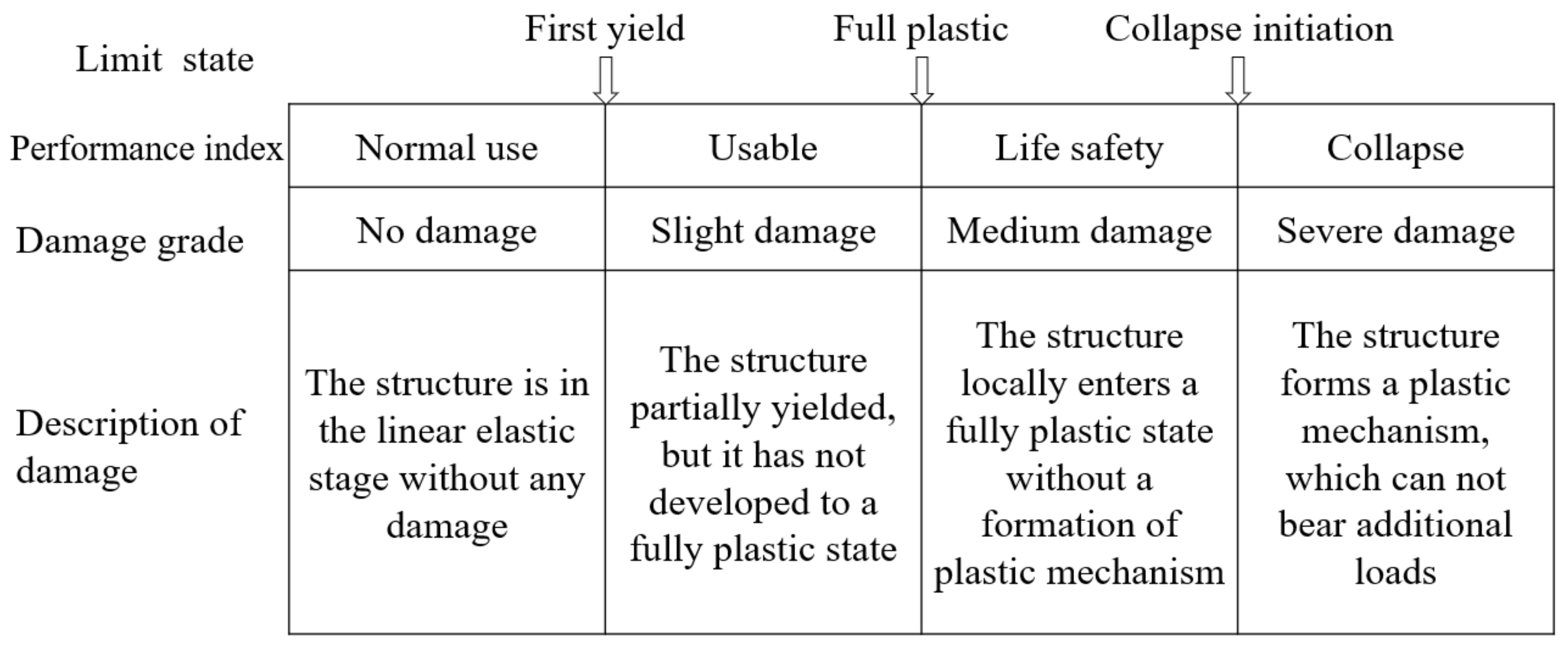
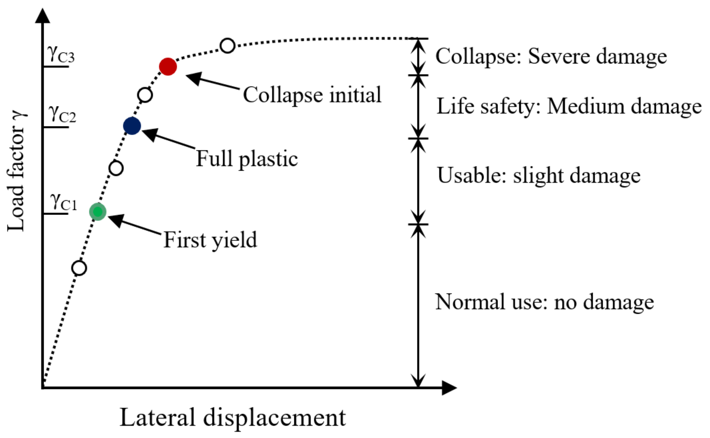
2.2. Nonlinear Assessment of Offshore Steel Trestles

This paper evaluates the capacity of the OST under the combined action of waves and currents. Wei et al. have defined three limit states, named first yield (FY), full plastic (FP), and collapse initiation (CI), according to the performance characteristics of the OST under stress [24]. The corresponding damage conditions are given in Figure 1.

Wei et al. have investigated the dynamic effect of an OST subjected to wave and current loads in the term of dynamic amplification factor (DAF) and found the DAF of the large wave is always smaller than 1.05 [24]. Neglection dynamic effect results in tiny influence on the nonlinear response of the OST. Therefore, the capacity of the three limit states of the OST, first yield (FY), full plastic (FP), and collapse initiation (CI), are calculated by the pushover analyses. The process of the pushover analyses is described as follows:

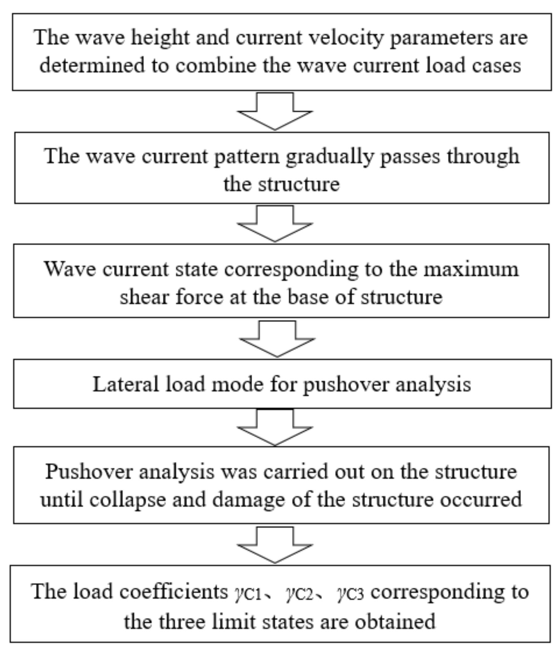
• Generating a regular wave train with the given wave height H_5% and the corresponding wave period T_5%, which is calculated as a function of wave height according to Valamanesh et al. [35], where g defines the acceleration of gravity:

$$T_{5\%}=11.1\sqrt{\frac{H_{5\%}}{1.86\mathrm{g}}}$$

(4)

2.

Using Equation (3) to calculate wave and current loads in the process of a complete phase of a regular wave (through-crest-through) stepping through the OST with a notably small-time interval. Define the wave and current loads corresponding to the maximum base shear, abbreviated as F_demand, in the process of wave stepping through the OST as a lateral load pattern.

3.

Pushover analyses of the OST are conducted based on the lateral load pattern. The pushover analyses will not stop until the OST collapses, taking the lateral displacement at the top of the OST as the classification index for three limit states. The base shear of the OST in three limit states corresponds to the capacity of the OST in three limit states, abbreviated as F_capacity. See Wei et el. [24,36] for more details of the process of pushover analyses.

This paper introduces the dimensionless load factor into the performance evaluation method to measure the capacity of the OST, which is defined as follows:

$$\gamma =\frac{F_{\mathrm{capacity}}}{F_{\mathrm{demand}}}$$

(5)

The load factors corresponding to the first yield (FY), full plastic (FP), and collapse initiation (CI) are γ_C1, γ_C2, and γ_C3, respectively. Figure 2 shows the relationship curve between the load factors and the lateral displacement at the top of the OST.

When γ_C = 1, the structure’s capacity to resist damage F_capacity (FY, FP, and CI) is just equal to the maximum base shear F_demand generated by a wave and current loads, and the structure is in the critical state of corresponding damage. When γ_C > 1, the capacity of the structure F_capacity is greater than the maximum base shear F_demand caused by wave and current loads, and the structure has no corresponding damage. When γ_C < 1, the corresponding damage occurs before the structure fully bears the given wave and current loads. Therefore, this paper uses the load factor to replace the response value corresponding to the OST limit state, which is more conducive to establishing the OST limit state function. The specific analysis process of this method is shown in Figure 3.

Because the evaluation method of the capacity of the OST under wave and current loads can realize the determination of the initial state of first yield (FY), full plastic (FP), and collapse initiation (CI), three limit state functions are still established based on these three limit states. Additionally, since the load factors corresponding to the three limit states can be obtained by this method, the three limit state functions Z can be rewritten as follows:

First yield:

$$Z_{C1}=R_1-S_1\left(H_{5\%},v\right)={\gamma }_{C1}-1=0$$

(6)

Full plastic:

$$Z_{C2}=R_2-S_2\left(H_{5\%},v\right)={\gamma }_{C2}-1=0$$

(7)

Collapse initiation:

$$Z_{C3}=R_3-S_3\left(H_{5\%},v\right)={\gamma }_{C3}-1=0$$

(8)

where R is the structural resistance; S is the load effect corresponding to wave height H_5% and current velocity v.

According to the basic form of a limit state function, we only need to build the kriging model, which characterizes the relationship between wave height, current velocity, and load factor. By judging whether the predicted value of the load factor corresponding to the sample points randomly selected by LHS is less than 1, the failure point in the sample points can be obtained, and the failure probability and reliability index of the structure can be obtained.

2.3. Kriging Model for Offshore Steel Trestles Subjected to Wave and Current Loads

The kriging model was initially derived and used to calculate deposit reserves and error estimates. The kriging method is a statistical prediction method based on the stochastic process. The corresponding relationship between the response value and the kriging model’s independent variable consists of the regression part $F\left(\beta ,x\right)$ and the random process $z\left(x\right)$. The specific model is as follows:

$$y(x)=F(\beta ,x)+z(x)$$

(9)

where $F\left(\beta ,x\right)$ is used to provide the global approximation of the kriging model, the mathematical expectation of $y\left(x\right)$; the mean value of $z\left(x\right)$ is 0, and the variance is ${\sigma }_z{}^2$. A random process with nonzero covariance provides an approximation to simulate local deviations, that is, local changes of $y\left(x\right)$. In engineering practice, the regression part generally adopts a polynomial form.

$$F(\beta ,x)=f{(x)}^{\mathrm{T}}\beta ={\beta }_1{f}_1(x)+{\beta }_2{f}_2(x)+\cdot \cdot \cdot +{\beta }_p{f}_p(x)$$

(10)

where $\beta$ is the regression coefficient of each function; p is the number of $f_i\left(x\right)$; and $f_i\left(x\right)$ is a polynomial function of variable x, which is similar to the polynomial form of the response surface method. For structures with a high nonlinear degree, such as OST, using a quadratic function as a regression model can obtain calculation results with high accuracy.

The covariance matrix $z\left(x\right)$ is:

$$\mathrm{Cov}[z(x_i),z(x_j)]={\sigma }_z^{2}R(\theta ,x_i,x_j)$$

(11)

where $x_i$ and $x_j$ are the i-th and j-th components of the training sample, respectively, and $R\left(\theta ,x_i,x_j\right)$ is the correlation function with a super parameter $\theta$, representing the spatial correlation between training sample points, which plays a decisive role in the simulation’s accuracy. There are many correlation functions, such as the exponential correlation function, Gaussian correlation function, Matérn-3/2, and Matérn-5/2. The most used function is the Gaussian correlation function, which is as follows:

$$R(\theta ,x_i,x_j)=\exp \left[-{\displaystyle \sum _{k=1}^{n_{\mathrm{dv}}}{\theta }_k{(x_{ik}-x_{jk})}^2}\right]$$

(12)

where $n_{\mathrm{dv}}$ is the number of known design variables and ${\theta }_k$ is the k-th element of vector $\theta$.

Given the training sample $S=\left[x_1,x_2,\cdot \cdot \cdot ,x_n\right]$ and its real response value $Y=\left[y_1,y_2,\cdot \cdot \cdot ,y_n\right]$ (n is the number of samples), the correlation matrix R of $n\times n$ and the regression partial matrix F of $n\times p$ are as follows:

$$R=\left[\begin{array}{ccc}R(x_1,x_1)& \cdots & R(x_1,x_n)\\ ⋮& \ddots & ⋮\\ R(x_n,x_1)& \cdots & R(x_n,x_n)\end{array}\right]$$

(13)

$$F=\left[\begin{array}{ccc}{f}_1(x_1)& \cdots & f_p(x_n)\\ ⋮& ⋮& ⋮\\ f_1(x_n)& \cdots & f_p(x_n)\end{array}\right]$$

(14)

The estimated value $\widehat{y}\left(x\right)$ of any point x can be expressed as:

$$\widehat{y}(x)=f^T(x)\tilde{\beta }+r^{\mathrm{T}}(x)R^{-1}(Y-F\tilde{\beta })$$

(15)

where $r\left(x\right)$ is the correlation vector between test point x and the sample point, which can be expressed as:

$$r(x)=[R(x,x_1),R(x,x_x),\cdot \cdot \cdot ,R(x,x_n)]$$

(16)

The maximum likelihood estimation factor is as follows:

$$\tilde{\beta }={(F^{\mathrm{T}}{R}^{-1}F)}^{-1}{F}^T{R}^{-1}Y$$

(17)

Under the Gaussian process assumption, the optimal kriging model is constructed by solving the unknown quantity $\theta$. According to the maximum likelihood estimation, it can be concluded that:

$${\sigma }^2=\frac{{(Y-F\tilde{\beta })}^T{R}^{-1}(Y-F\tilde{\beta })}{n}$$

(18)

Among them, $\theta$ can be obtained by solving the following optimization problems:

$$\underset{{\theta }_k>0}{{\displaystyle \max }}-\frac{[n\ln ({\sigma }^2)+\ln |R|]}{2}$$

(19)

A certain amount of available information is required to develop the kriging model. Therefore, it is necessary to select a certain number of sample points in a specific design space range and conduct numerical experiments. LHS is a multi-dimensional stratified sampling method. Compared with MCS, LHS is designed to accurately reconstruct the input distribution by sampling with fewer iterations, providing more comprehensive sample information to establish the kriging model. The basic principles of LHS are as follows:

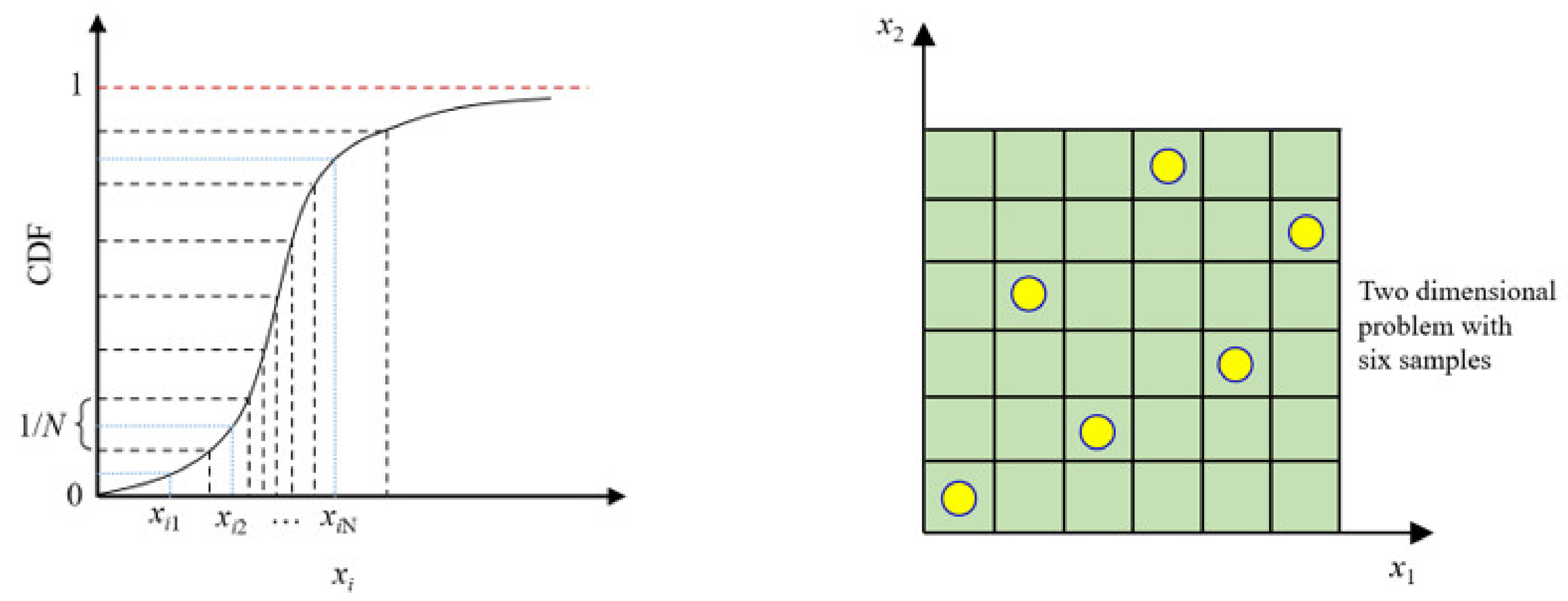
• Define the sampling number N participating in the computer operation;
• Divide each input equally into N columns, where $x_{i0}<x_{i1}<x_{i2}<x_{i3}\dots <x_{in-1}<x_{in}<x_{in+1}<\mathrm{\dots }<x_{iN}$, and $P(x_{in}<x<x_{in+1})=\frac{1}{N}$;
• Select only one sample for each column, and each column’s bin position is random.

LHS avoids the collapse of sample data and can use fewer samples to represent the overall distribution of parameters, which has a good filling for the sampling space, as shown in Figure 4.

Suppose a parameter A obeys a Gaussian normal distribution, the average value of the ideal distribution is 1.5, and the standard deviation is 2.0. LHS and MCS were used to obtain samples with a capacity of 1800, and the mean and variance of samples were calculated. A total of 20 simulations were performed. Figure 5a,b show the fluctuation of the sample mean and variance with simulation times, respectively. The results show that LHS’s statistical parameters are more accurate and stable than those obtained by MCS.

2.4. Reliability Analysis Process

The analysis can proceed as follows:

• According to the practical problems of OSTs, the influencing factors of the capacity of OSTs are determined; namely, random variable $\left(X_1,X_2,\cdots ,X_j\right)$ and the limit state of OST are defined;
• According to the distribution function of the random variable $\left(X_1,X_2,\cdots ,X_j\right)$, LHS is used to sample random variables and m×j dimension random variable samples are generated;
• The random variable samples are substituted into the finite element model to generate the corresponding analysis conditions and the corresponding response values of the OST’s limit state are obtained;
• The kriging model of the response value in accordance with a certain accuracy is constructed by using the random variable samples and the response values;
• Again, LHS is used to extract n×j dimensional random variable samples, and the predicted response values of each random variable sample are obtained by substituting them into the kriging model;
• The predicted response value is substituted into the limit state equation Z. If Z is less than 0, it is the failure point. Assuming that the number of failure points is k, the failure probability is P_f = k/n. The failure probability can be expressed as:

$$P_{\mathrm{f}}=\frac{1}{n}{\displaystyle \sum _{i=1}^{n}I(Z)}$$

(20)

When Z < 0, I(Z) = 1; when Z < 0, I(Z) = 0. Then, the reliability index of OST is:

$$\beta =-{\Phi }^{-1}(P_{\mathrm{f}})$$

(21)

where Φ is the standard normal distribution function.

As an approximate fitting model, the kriging model can have some errors with the real model. To test the fit effect of the kriging model, it is mainly judged by the Theil inequality coefficient, which can be calculated as follows:

$$\tau =\frac{\sqrt{\frac{1}{n}{\displaystyle \sum _{i=1}^n{(y_i-{\widehat{y}}_i)}^2}}}{\sqrt{\frac{1}{n}{\displaystyle \sum _{i=1}^n{\widehat{y}}_i{}^2}}+\sqrt{\frac{1}{n}{\displaystyle \sum _{i=1}^n{y}_i{}^2}}}$$

(22)

where n is the number of samples; $y_i$ is the calculated actual value of the i-th sample point; ${\widehat{y}}_i$ is the predicted value of the kriging model of the i-th sample point; and $\tau$ is the Theil inequality coefficient, which is between 0 and 1, and the closer to 0, the better the fitting effect is.

This paper’s method only pays attention to the randomness of load parameters, that is, the randomness of wave and current parameters $\left(X_{wave},X_{current}\right)$ in the reliability analysis of OST. The kriging models proposed above are compiled using ooDACE toolbox of the software MATLAB (Mathworks Inc., Natick, MA, USA) [37].

3. Calculation Example

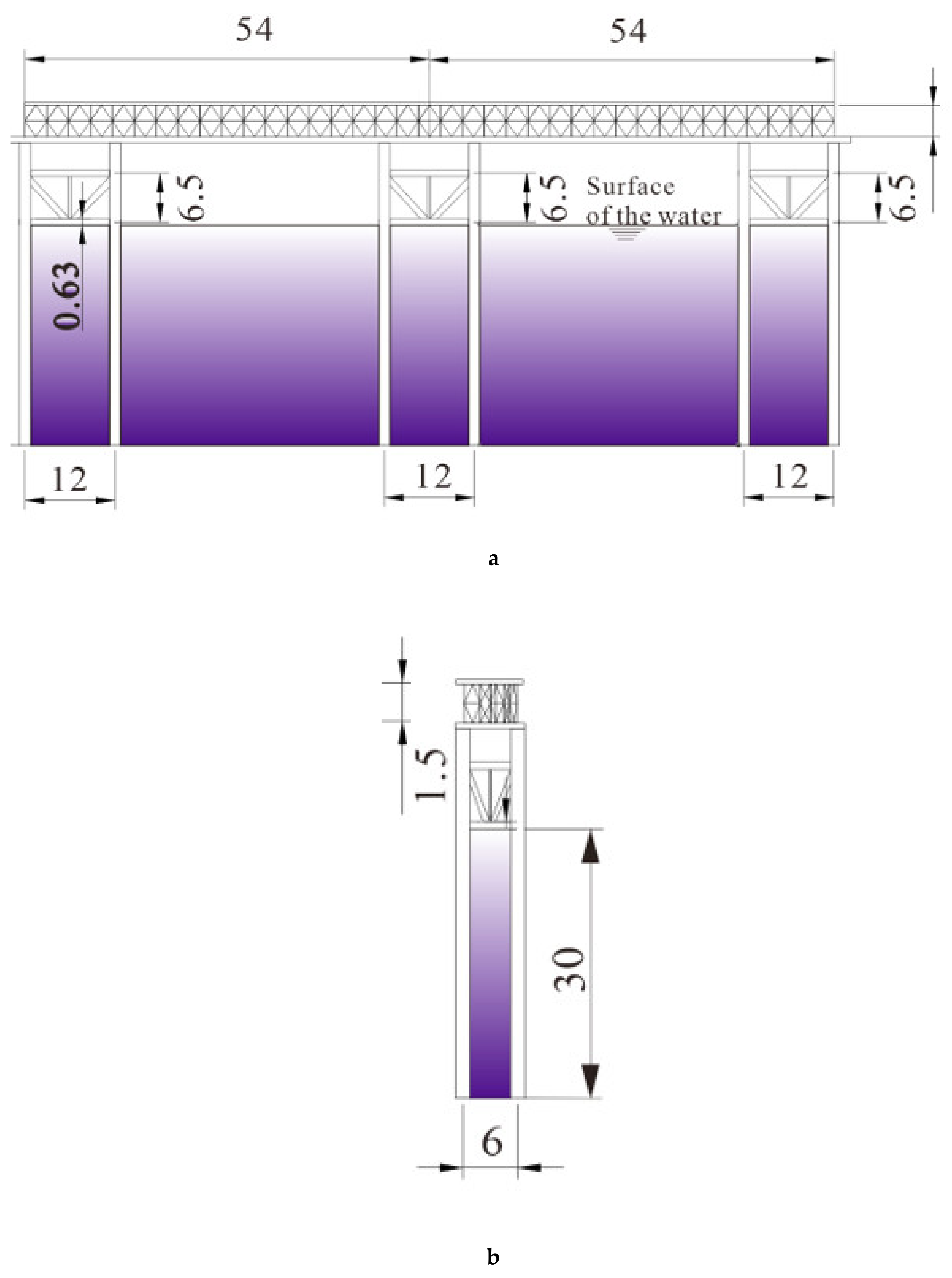
3.1. Example Structure

The OST of the Pingtan Strait Rail-cum-road Bridge is taken as the example structure, as shown in Figure 6. The OST is a two-span continuous beam structure with a length of 54 + 54 m, a width of 6 m, and a water depth of 25 m. The height from the bridge deck to the seabed is 42 m, and the clearance of the OST is 15 m. The bridge deck is fixed by bailey beams, which are supported by beams. The steel pipe pile and the supporting frame are welded together to form a jacket-type support system. The steel pipe pile is embedded in the seabed rock. The bailey beam’s height is 1.5 m, and the distance between adjacent bailey plates is 1.5 m. The height of the steel pipe pile is 40 m, the diameter is 1.5 m, and the spacing of the steel pipe pile is 12 m. The supporting frame’s height is 6.5 m, the diameter of the upper and lower transverse bracing and diagonal bracing is 0.63 m, and the diameter of the vertical brace is 0.35 m. The thicknesses of the steel pipe pile and supporting frame are 16 mm and 10 mm, respectively. The bailey beam is made of Q345 steel, the steel pipe pile is made of Q235 steel, and the bridge deck is made of 16 Mn steel. The specific dimensions are shown in Figure 6. The measured wave and current parameters in the bridge site’s sea area are shown in

Table 1. Measured wave and current parameters at the bridge site.

Return Period (year)	Environmental Parameters
	v (m/s)	H5% (m)
10	2.46	5.44
20	2.52	6.22
100	2.66	7.29

.

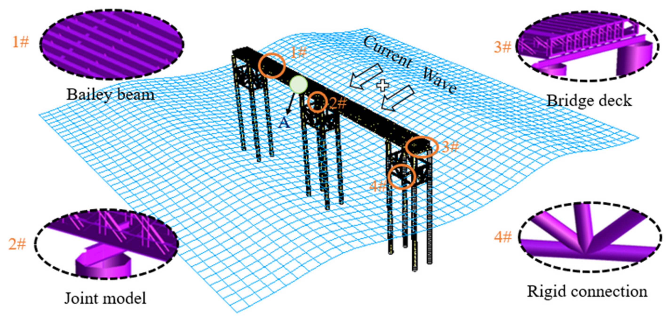
3.2. Establishment of the Finite Element Model

The three-dimensional numerical model of the OST is established using the finite element software USFOS (SINTEF marintek, Oslo, Norway and the Norwegian University of Science and Technology, Trondheim, Norway) as shown in Figure 7. Nonlinear beam elements are used to simulate the bailey beam, jacket, and steel pipe pile. The plastic hinge model is used to simulate the nonlinearity of the bar material. The elastic–plastic model considering strain strengthening is adopted for the mechanical behavior of the plastic hinge. The plastic hinge is automatically inserted into the two ends or the beam element’s middle point according to the element’s plastic development. The four-point shell element model is used to establish the bridge deck. A rigid connection is adopted between the bailey frame and steel pipe column, and a rigid connection is still adopted between the superstructure and substructure. The mass of guardrail and vehicle load on the bridge deck is considered by increasing the bridge deck’s thickness. The bottom of the steel pipe pile is consolidated and constrained. The nonlinear geometric effects of large displacement and strain are considered. In this paper, the waves and the currents are set in the same direction and along the transverse direction of the OST.

The local elastic–plastic deformation of tubular joints occurs when subjected to large external forces. However, the traditional rigid joint connection method assumes that the local elastic deformation and plastic deformation after the yielding of tubular joints are not considered in the stress analyses. This paper uses MSL joint model, developed by MSL Engineering Ltd. in County Cork, Ireland [38] to simulate the plastic behavior in the OST joints. The simulation method models the pipe joint’s nonlinear deformation after being stressed by a nonlinear spring between the chord skin and the chord centerline.

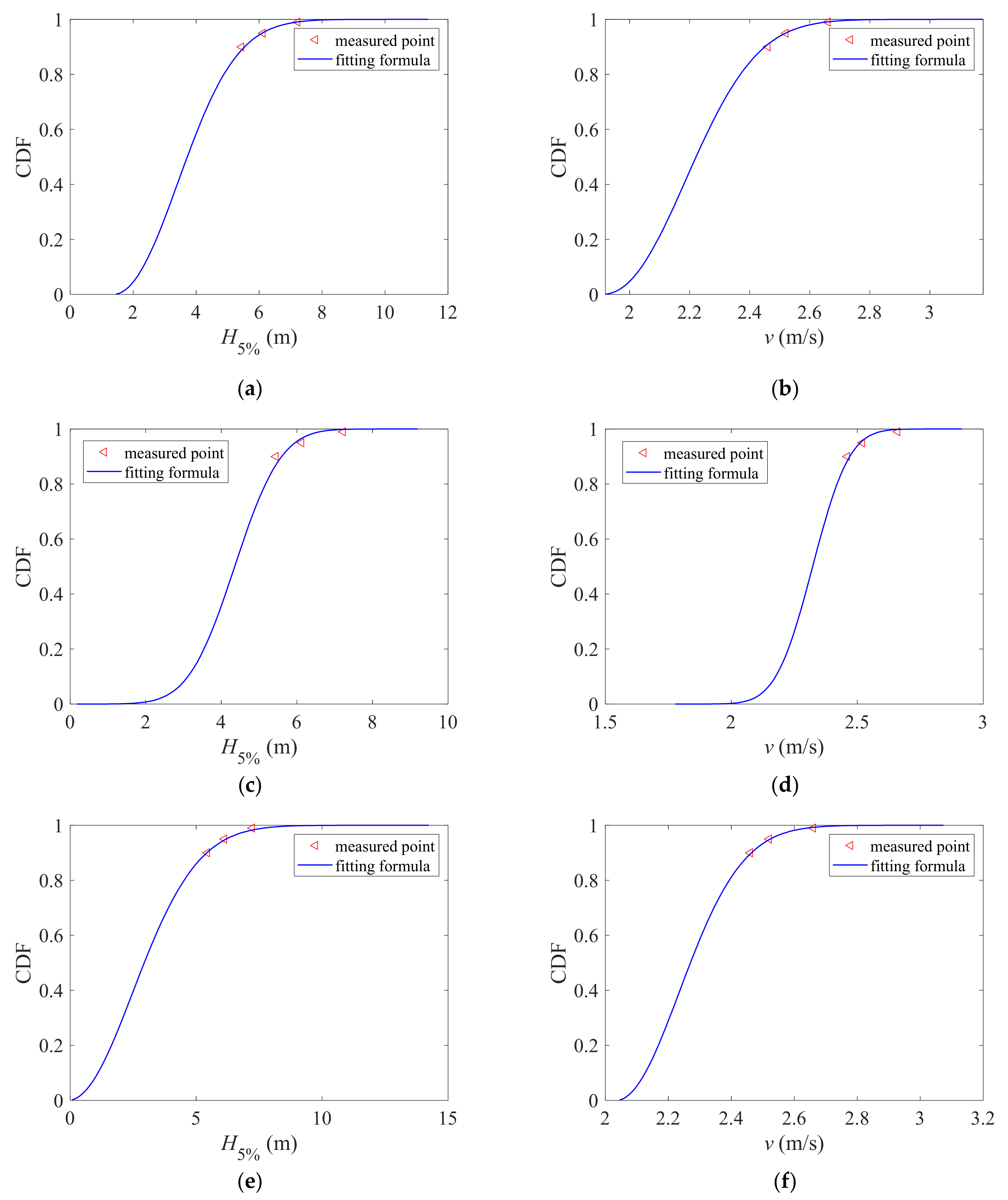
3.3. Stochastic Model of Wave and Current Conditions

Since there are only three sets of wave and current conditions, three distributions are used for the comparison of the probability distribution of wave and current parameters of the OST. They are the three-parameter Weibull extreme value distribution, the Gaussian distribution, and the Rayleigh distribution.

The three-parameter Weibull extreme value distribution model was proposed by the South China Sea Institute of Oceanography, Chinese Academy of Sciences. The three-parameter Weibull extreme value distribution function is as follows:

$$F(x)=1-\exp \left[1-{\left(\frac{x-\mu }{\alpha }\right)}^{\xi }\right]$$

(23)

where α is the scale parameter, μ is the position parameter, and ξ is the shape parameter.

The Gaussian distribution function is as follows:

$$F(x)=\frac{1}{\sigma \sqrt{2\mathsf{\pi }}}\exp (-\frac{{(x-\mu )}^2}{2{\sigma }^2})$$

(24)

where μ is the mu parameter, and σ is the sigma parameter.

The Rayleigh distribution function is as follows:

$$F(x)=1-\exp \left(-\frac{x^2}{2}\right){\sigma }^2$$

(25)

where σ is the sigma parameter.

The extreme value x_p of environmental load parameters with the n-year return period can be determined according to the probability distribution function of load parameters. The probability of occurrence of environmental load parameters with the n-year return period is 1/n.

$$P(x>x_p)=1-F(x_p)=\exp \left[1-{\left(\frac{x_p-\mu }{\alpha }\right)}^{\xi }\right]=\frac{1}{n}$$

(26)

Then, the extremum quantile x_p can be expressed as follows:

$$x_p=\alpha {(\ln n)}^{\frac{1}{\xi }}+\mu$$

(27)

Referring to the measured wave and current parameters in the bridge site’s sea area (Table 1), the distribution of wave height and current velocity is shown in Figure 8. The three-parameter Weibull extreme value distribution function, Gaussian distribution function and Rayleigh distribution function of wave height and the current velocity are as follows:

$$F(H_{5\%})=1-\exp \left[1-{\left(\frac{x-1.4}{2.82}\right)}^{2.106}\right]$$

(28)

$$F(v)=1-\exp \left[1-{\left(\frac{x-1.91}{0.3729}\right)}^{2.2}\right]$$

(29)

$$F(H_{5\%})=\frac{1}{0.97\sqrt{2\mathsf{\pi }}}\exp (-\frac{{(x-4.4)}^2}{2\cdot {(0.97)}^2})$$

(30)

$$F(v)=\frac{1}{0.115\sqrt{2\mathsf{\pi }}}\exp (-\frac{{(x-2.329)}^2}{2\cdot {(0.115)}^2})$$

(31)

$$F(H_{5\%})=1-\exp \left(-\frac{x^2}{2}\right)*{2.56}^2$$

(32)

$$F(v)=1-\exp \left(-\frac{{(x-2.04)}^2}{2}\right)*{0.2}^2$$

(33)

4. Reliability Analysis Results

4.1. Verification of the Proposed Method

When constructing the kriging model, it is assumed that the wave height and current velocity parameters are uniformly distributed. The sampling range of wave height and the current velocity is based on the actual distribution range of wave height and current velocity; that is, the sampling range of wave height is (2 m, 12 m), and the sampling range of current velocity is (1 m/s, 4 m/s). To verify the proposed method, this paper selects 500 samples of wave height and current velocity according to the uniform distribution type and distribution range. The predicted values of 500 samples are obtained by using the kriging model. The Theil inequality coefficient of the kriging model is calculated from the actual values and the predicted values obtained by the kriging model. When the Theil inequality coefficient is less than 0.01, the kriging model’s prediction accuracy can be considered to meet the requirements.

The kriging models corresponding to three limit states with specific sample numbers of 100 are given in Figure 9, Figure 10 and Figure 11, as well as the comparison between actual and predicted load factor values. The figure shows that the kriging model is consistent with the original surface and the predicted value is equal to the actual value. The Theil inequality coefficient of the kriging model is less than 0.01, which verifies the accuracy of the method.

Table 2. Failure probability and reliability index corresponding to three limit states of OST using the three-parameter Weibull extreme value, Gaussian, and Rayleigh distribution for fitting of wave and current parameters.

Limit State	Three-Parameter Weibull Extreme Value		Gaussian		Rayleigh
	Failure Probability Pf (%)	Reliability Index β	Failure Probability Pf (%)	Reliability Index β	Failure Probability Pf (%)	Reliability Index β
FY	0.4887	2.5837	0.0812	3.1516	1.6576	2.1302
FP	0.1078	3.0682	0.0024	4.0698	0.6576	2.4796
CI	0.0348	3.3913	0.0011	4.2285	0.2659	2.7871

gives the failure probability and reliability index of the three limit states of the OST under three different distributions of wave and current. Table 2 shows that the failure probability of the OST gradually decreases with the increase of the limit state and its corresponding reliability index increases with the increase of the limit state. Different distributions of wave and current result in different failure probability and reliability index of the three limit states of the OST. The result of using the Rayleigh distribution will have the highest failure probability, and the use of Gaussian distribution will have the lowest failure probability. This is due to the use of Rayleigh distribution for fitting of wave and current distribution, resulting in more large waves and rapid current velocities. The failure probability obtained for limit state FY is relatively high; because the partial yielding in the definition of FY is more likely to occur, it does not affect the normal use of the OST. As the distributions of both wave and current conditions affect the reliability significantly, it is necessary to have more measured data to fit the distributions and make the results of reliability more realistic.

4.2. Comparison of MCS, LHS, and Kriging Model

The failure probability and reliability index of OST are calculated using the other two widely used reliability analysis methods, MCS and LHS, to reflect the accuracy and efficiency of the reliability analysis method for OST based on the kriging model. Three-parameter Weibull extreme value distribution is used for sampling. Three methods are defined as follows:

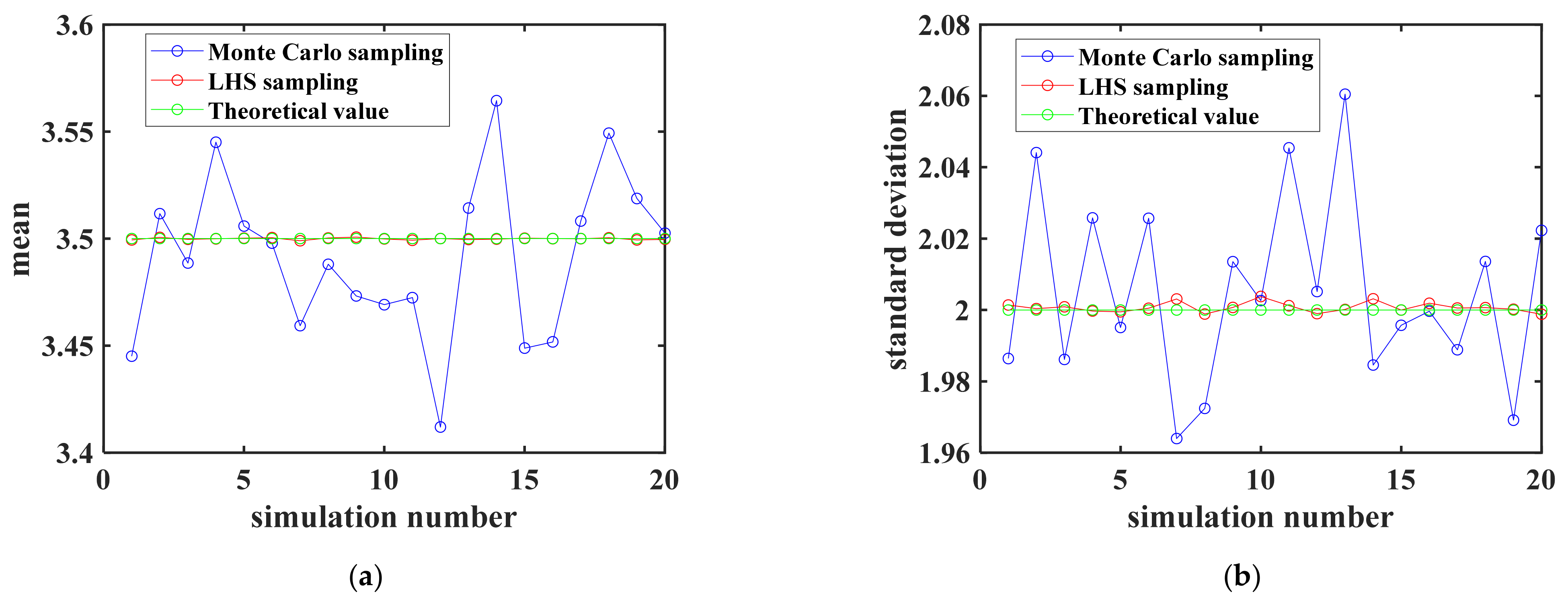
• MCS is used to randomly select a large number of samples of wave height and current velocity that obey the three-parameter Weibull extreme value distribution, all samples are analyzed by the finite element method one by one, and the load factors corresponding to the three limit states of the OST are obtained. The number of failure samples whose load factor is less than one is counted for each limit state. Finally, the ratio of failure events to the whole sample is calculated. The failure probability and reliability index corresponding to the three limit states of the OST are obtained.
• The second method is LHS. The only difference between LHS and MCS is that the sampling method is different. LHS is used in the sampling of wave height and current velocity samples.
• For the kriging model, it is worth noting that the kriging model constructed in this paper uses LHS twice with different purposes. The first time LHS is used to extract a certain sample number to establish a kriging model, the second time LHS is used to extract the load factors to calculate reliability index and failure probability.

Table 3. Comparison of reliability calculation time and results using MCS, LHS, and the kriging model.

Calculation Method	Limit State	Finite Element Analyses/Time	Analysis Time/Hour	Failure Probability Pf (%)	Reliability Index β	Relative Error (%)
MCS	FY	1.15 × 105	1437.5	0.4583	2.6058	—
	FP			0.0983	3.0954	—
	CI			0.0313	3.4201	—
LHS	FY	8.5 × 104	1062.5	0.4878	2.5843	0.0083
	FP			0.1000	3.0902	0.0017
	CI			0.0341	3.3966	0.0069
Kriging model	FY	100	1.25	0.4887	2.5837	0.0085
	FP			0.1078	3.0682	0.0088
	CI			0.0348	3.3913	0.0084

Note: The average calculation time for each finite element is 45 s.

summarizes the reliability results obtained by the three methods and compares the total analysis time spent by the three methods in solving the reliability results. The whole analysis time is mainly the calculation time of all finite element analyses. The time spent in other processes is generally less than ten minutes, which can be ignored, such as sample sampling and failure sample quantity statistics.

Table 3 shows that when MCS is used to calculate the reliability of OST directly, 1.15×10⁵ finite element analyses are needed to obtain an accurate approximate solution of the structural reliability. The analysis time is approximately 1437.5 h. When the LHS is used instead of the MCS, the calculation amount of finite element analyses can be effectively reduced, the time saved is approximately 26%, and the relative error of the reliability index is within 1%. The LHS is better than the MCS in the reliability calculation. The reliability analysis method of OST based on the kriging model proposed in this paper only needs 100 finite element analyses to obtain more accurate reliability results. The analysis time is approximately 1.25 h. Compared with MCS and LHS, the calculation time is reduced by three orders of magnitude, and the relative error of the reliability index is within 0.01%.

4.3. Influence of Sample Number on the Prediction Accuracy of the Kriging Model

In theory, the more samples that are extracted when constructing the kriging model, the higher the accuracy of the kriging model. However, if the number of samples is too large, the number of finite element analyses inevitably increases, which affects the calculation efficiency and fails to reflect the efficiency of the dynamic kriging model. To improve the calculation efficiency, it is necessary to determine the appropriate sample size using LHS. This section analyzes the impact of sample size on the accuracy of the kriging model. Previous studies have shown that the number of samples required for constructing the kriging model should not be less than 30. Therefore, the number of samples is selected to be 40, 60, 80, 100, and 120.

Table 4. Theil inequality coefficients of the kriging model corresponding to three limit states under different sample numbers.

Limitstate	Sample Number
	40	60	80	100	120
First yield	0.0656	0.0359	0.0117	0.0076	0.0066
Full plastic	0.0513	0.0413	0.0123	0.0074	0.0059
Collapse initiation	0.0448	0.0263	0.0126	0.0085	0.0077

shows the kriging model’s Theil inequality coefficient corresponding to three limit states under different sample numbers. Table 4 clearly shows that with the increase in sample number, the Theil inequality coefficient of the kriging model corresponding to the three limit states gradually decreases; that is, the prediction accuracy increases continuously. When the number of samples is 100, the kriging model’s Theil inequality coefficients corresponding to three limit states are less than 0.01, which meets the prediction accuracy. Therefore, a 100 sample number is used to construct the kriging model.

After obtaining the kriging model of the relationship between wave height, current velocity, and load factor, to obtain the failure probability and reliability index of OST, we need to extract a certain number of load factors using LHS again. Although LHS can represent the random distribution characteristics of parameters with only a few samples, it may not obtain an accurate reliability index and failure probability with a few samples. Therefore, it is necessary to explore the influence of the sample number on the failure probability of the OST to determine the appropriate sample number in advance. The sample size ranges from 5000 to 200,000, and the step size is 5000. The sample of wave height and current velocity obey the three-parameter Weibull extreme value distribution.

Figure 12 shows the variation in failure probability with the number of samples corresponding to the three limit states of the OST. Figure 12 shows that when the number of samples is small, the failure probability corresponding to each limit state fluctuates greatly. It is mainly because of the large wave height and current velocity required for the structure’s FY, FP, and CI. Suppose the number of samples is too small. In that case, the number of Latin hypercube delamination intervals is less. The wave height or current velocity range corresponding to the equal cumulative probability interval is large, resulting in the randomness of large wave height or high current velocity being sampled. In addition, when the number of samples reaches 35,000, 55,000, and 85,000, the failure probability corresponding to the FY, FP, and CI of OST fluctuates slightly, and the fluctuation ranges are ±0.5%, ±1%, ±1.5%, respectively. As demonstrated by the blue dotted lines in the figure, the failure probability tends to be stable. It should be noted that the size of the failure probability is inversely proportional to the number of samples corresponding to the stable failure probability. That is, the greater the failure probability is, the fewer samples need to be calculated. To ensure that the failure probability corresponding to the three limit states can reach high accuracy and reduce the sampling process, the sample size is 85,000.

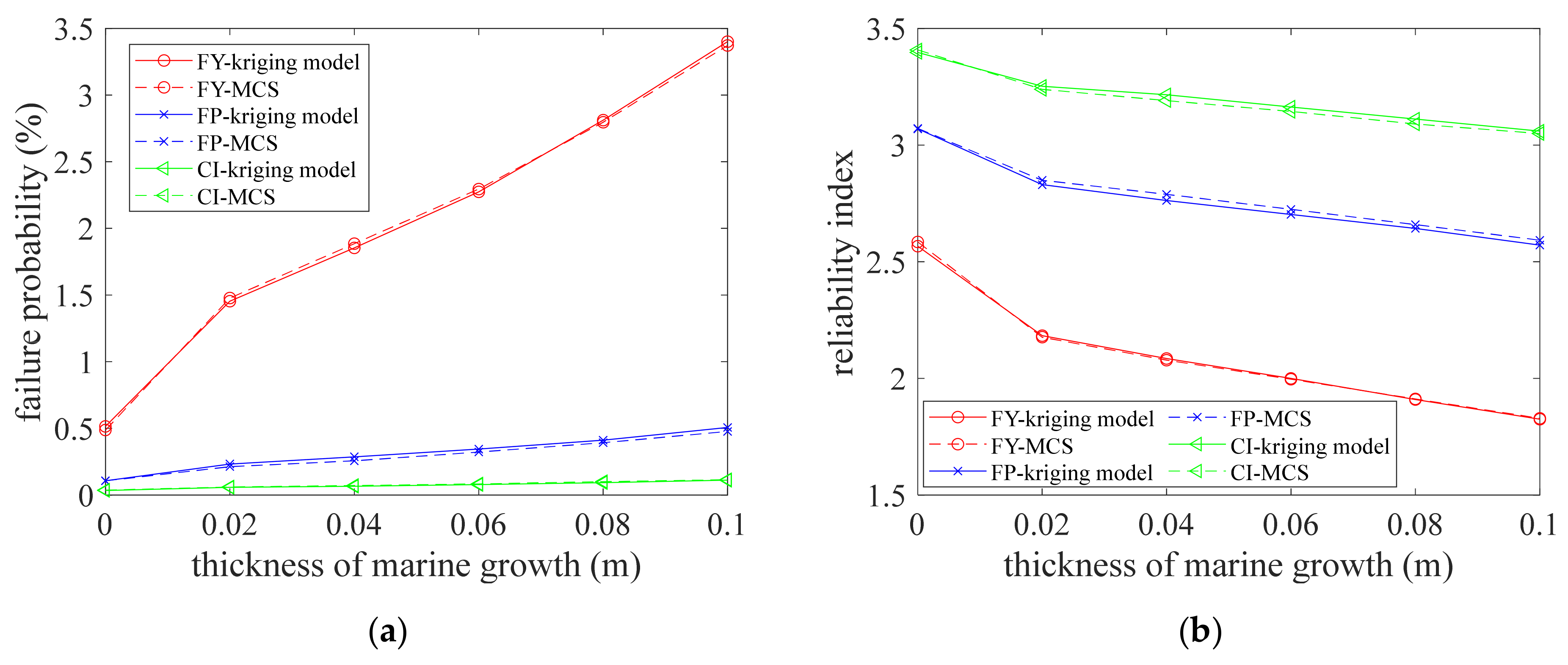
4.4. Influence of Marine Growth on the Reliability Analysis of the OST

A measurement of marine growth on a platform in the China South Sea demonstrates that the annual marine growth thickness can be as large as 10 mm, when the water depth is smaller than 50 m [39]. Studies have shown that marine growth increase wave and current loads on the OST by increasing the hydrodynamic radius and the roughness of the steel pipe pile and changing the hydrodynamic coefficient, and thereby affecting the capacity of the OST [40]. To understand the influence of marine growth on the reliability of the OST, the proposed kriging model is used to analyze the reliability of the OST under different thicknesses of marine growth.

The load factors ${\gamma }_{C1,C2,C3}\left(t_m,H_{5\%},v\right)$ of three limit states corresponding different thickness of marine growths have an approximately linear relationship with the load factors γ corresponding to three limit states of the OST. This relationship does not include the case where the thickness of the marine growth t_m = 0 m, because the hydrodynamic coefficient of t_m = 0 m is set up as 1.2 for C_D and 2.0 for C_M, while the hydrodynamic coefficient is set up as 1.4 for C_D and 1.8 for C_M when t_m is not 0 m [41]. Therefore, based on the condition of t_m = 0.02 m, the load factors γ_C1, γ_C2, and γ_C3 with any thickness of marine growth of the OST under wave and current loads can be calculated according to the following equation:

$${\gamma }_{\mathrm{C}1,\mathrm{C}2,\mathrm{C}3}(t_{\mathrm{m}},H_{5\%},v)={\lambda }_{{\gamma }_{\mathrm{C}1},{\gamma }_{\mathrm{C}2},{\gamma }_{\mathrm{C}3}}(t_{\mathrm{m}})\times {\gamma }_{\mathrm{C}1,\mathrm{C}2,\mathrm{C}3}(0.02,H_{5\%},v)$$

(34)

where ${\lambda }_{{\gamma }_{\mathrm{C}1},{\gamma }_{\mathrm{C}2},{\gamma }_{\mathrm{C}3}}\left(t_m\right)$ represents the relationship between ${\gamma }_{\mathrm{C}1,\mathrm{C}2,\mathrm{C}3}\left(t_m,H_{5\%},v\right)$ and ${\gamma }_{\mathrm{C}1,\mathrm{C}2,\mathrm{C}3}\left(0.02,H_{5\%},v\right)$, the correlation equation is as follows [42]:

$${\lambda }_{{\gamma }_{\mathrm{C}1},{\gamma }_{\mathrm{C}2},{\gamma }_{\mathrm{C}3}}=-1.45t_{\mathrm{m}}+1.027$$

(35)

As the above relationship does not include the case of t_m = 0 m, when calculating the failure probability and reliability index corresponding to the thickness of different marine growths, it is necessary to construct the kriging model corresponding to the three limit states of the OST when the thickness of the marine growth is at first 0.02m. Based on the kriging model of t_m = 0.02 m combined with Equation (35), the kriging model corresponding to the three limit states of the OST under different thicknesses (0.04 m, 0.06 m, 0.08 m, and 0.1 m) of marine growths is constructed, and then the corresponding reliability index is obtained using the LHS. Figure 13 shows the reliability index and failure probability of the OST under different marine growth thicknesses obtained by the kriging method and MCS.

It can be observed from Figure 13 that the reliability indexes of the OST under different marine growth thicknesses, calculated by the kriging method and MCS, are in good agreement with the results, and the relative error is within 1.5%. In the process of the OST from having no marine growth to having marine growths, its failure probability and reliability indexes are significantly increased and decreased, respectively. As the thickness of marine growths increases, the failure probability of the OST increases linearly, and the corresponding reliability indicators gradually decrease linearly.

Table 5. The degree of reliability index reduction under the influence of marine growth of the OST.

Limit State	Failure Probability Pf/%		Reliability Index β		Reduction Degree of β/%
	tm= 0 m	tm= 0.1 m	tm= 0 m	tm= 0.1 m
First yield	0.489	3.660	2.606	1.792	31.23
Full plastic	0.108	0.547	3.095	2.545	17.79
Collapse initiation	0.035	0.106	3.420	3.073	10.15

shows the change of the reliability index of the OST with the increase of the thickness of the marine growth from 0 to 0.1m. It can be observed from Table 5 that with the influence of marine growths, the failure probability corresponding to three limit states of the OST will be significantly increased, and the corresponding reliability index will be significantly reduced. Among them, the degree of reliability index reduction is as follows: First yield (31.23%) > Full plastic (17.79%) > Collapse initial (10.15%). Marine growths will affect the fatigue behavior of the OST, and thus affect the capacity of the OST. However, this aspect is not considered in this paper and is worth considering in future work.

5. Conclusions

Based on the kriging model and LHS, a reliability analysis method for OST is proposed in this paper. The reliability index of the OST used in the Pingtan Strait Rail-cum-road Bridge is solved based on this method. Three different distributions are used for comparison of the results of failure probability and reliability index. The reliability calculation results and analysis time of this method are compared with MCS and LHS. The sample number’s influence on the prediction accuracy and reliability index of the kriging model for the reliability analysis of OST is discussed. In addition, the influence of marine growth on the reliability analysis of the OST is discussed using the kriging model and MCS. The main conclusions are described as follows:

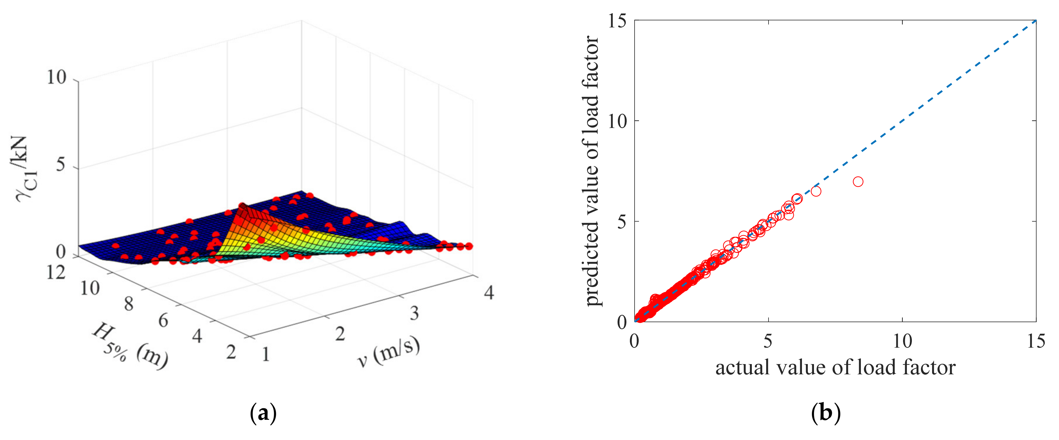
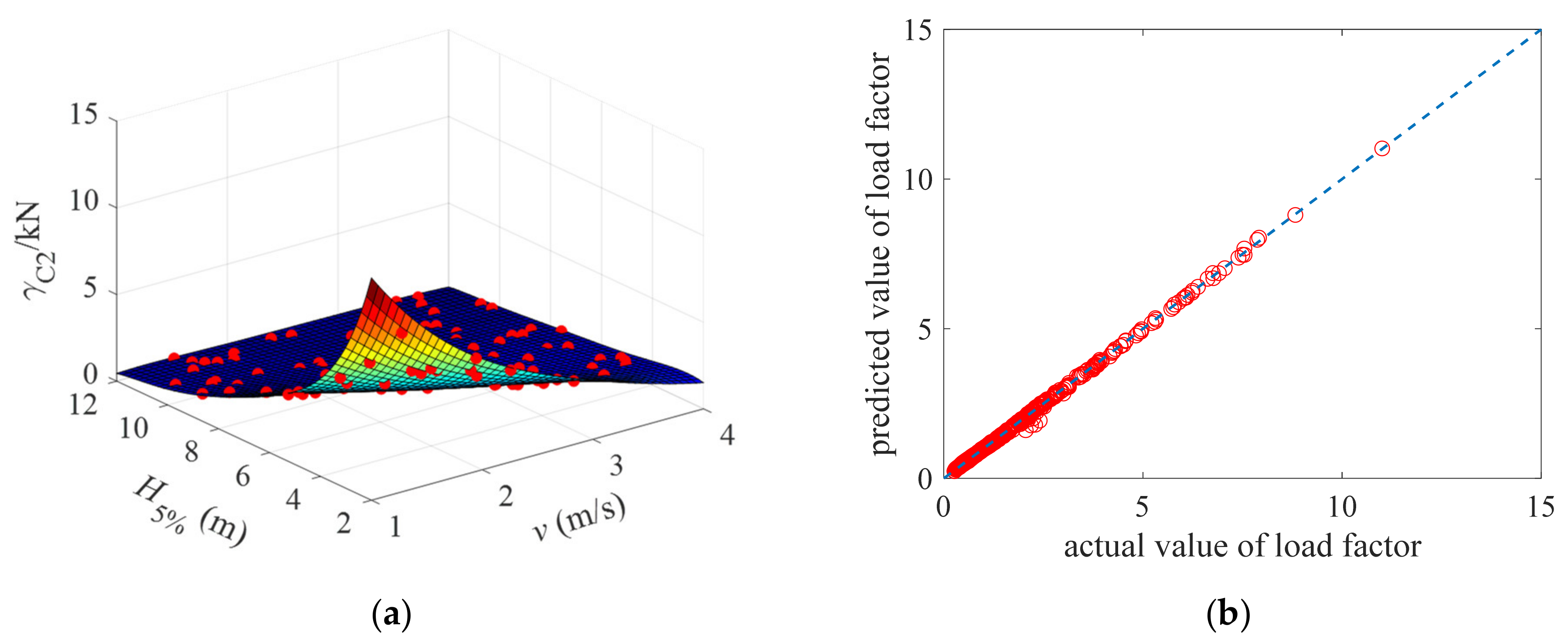
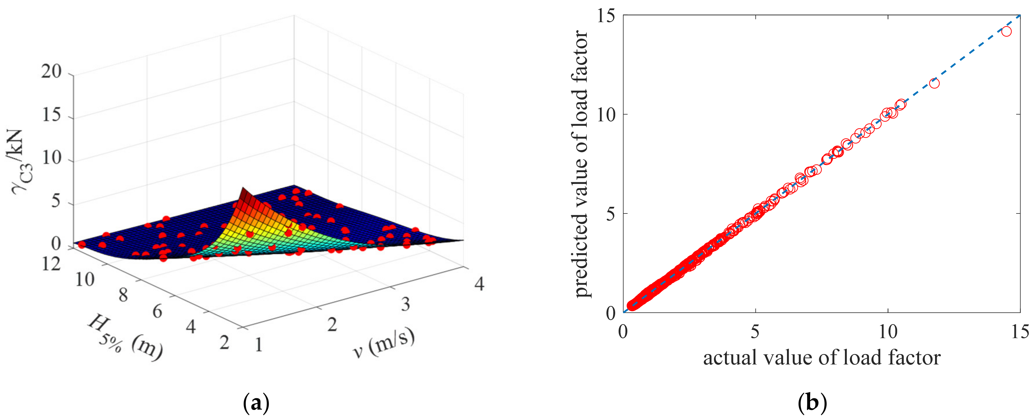
• The kriging model is constructed assuming that the wave height and current velocity parameters are uniformly distributed. The sampling range of wave height is (2 m, 12 m), and the sampling range of current velocity is (1 m/s, 4 m/s). A total of 500 samples of wave height and current velocity are selected according to the uniform distribution type and distribution range to verify the proposed method. The Theil inequality coefficient of the kriging model is less than 0.01, which verifies the accuracy of the method. The failure probability of the OST gradually decreases with the increase of the limit state, all less than 0.600%, and its corresponding reliability index gradually increases with the increase of the limit state, all greater than 2.5. Different distributions of wave and current result in different failure probability and reliability index of the three limit states of the OST. The result of using the Rayleigh distribution will have the highest failure probability, and the use of Gaussian distribution will have the lowest failure probability.
• Compared with MCS and LHS, the reliability analysis method based on the kriging model can obtain the reliability index of OST efficiently and accurately. The analysis time is approximately 1437.5 h and 1062.5 h when using MCS and LHS, while the calculation time is approximately 1.25 h when using the kriging model. Compared with MCS and LHS, the calculation time is reduced by three orders of magnitude. Compared with MCS, the relative error of the reliability index using the kriging model is within 0.01%, which shows the accuracy of the kriging model.
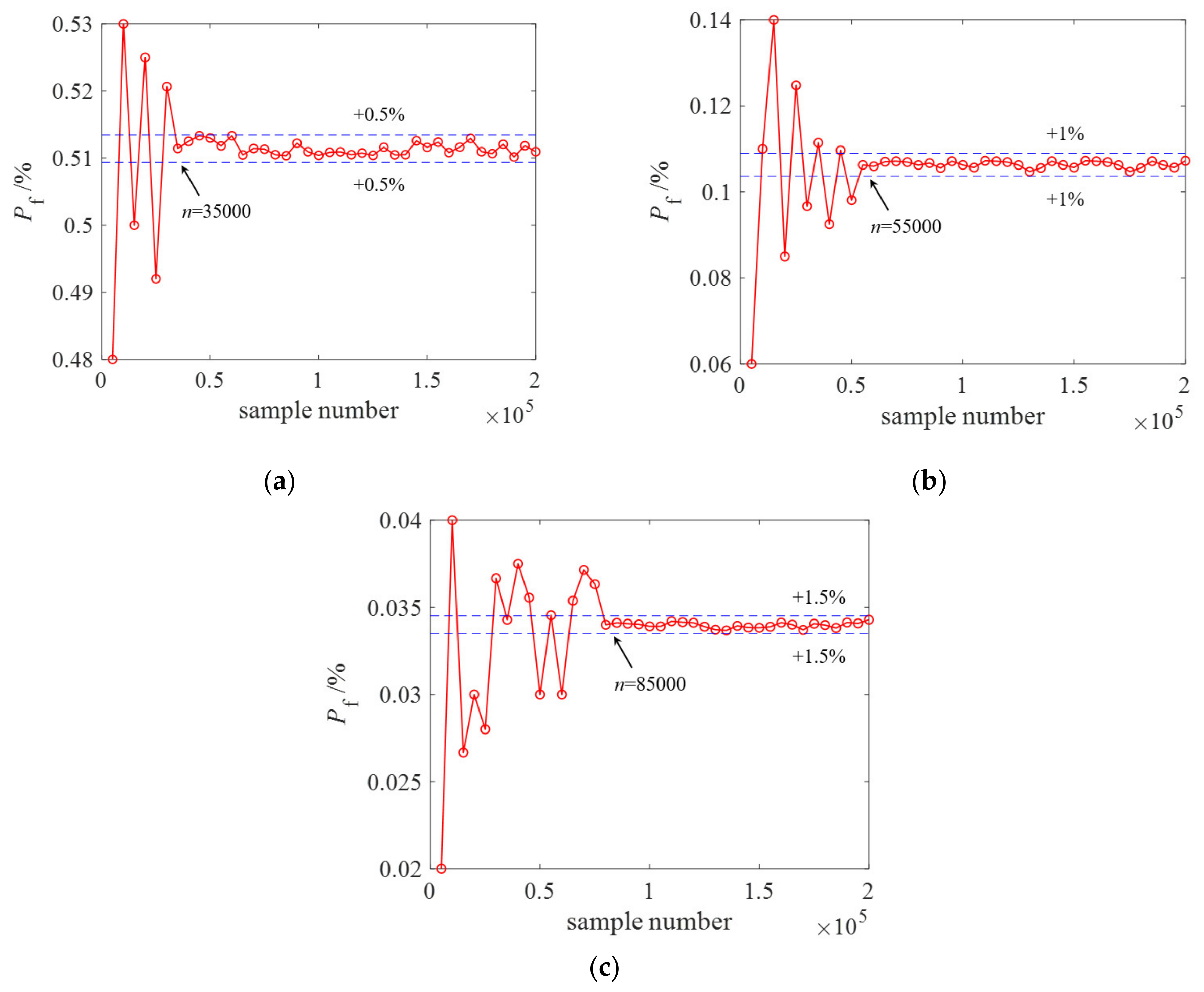
• When constructing the kriging model, the sample number is selected to be 40, 60, 80, 100, and 120. With the increase in sample number, the Theil inequality coefficient of the kriging model corresponding to the three limit states gradually decreases; that is, the prediction accuracy increases continuously. When the number of samples is 100, the kriging model’s Theil inequality coefficients corresponding to three limit states are less than 0.01, which meets the prediction accuracy. When extracting a certain number of load factors using LHS to obtain an accurate reliability index and failure probability, the sample size ranges from 5000 to 200,000 with the step size of 5000 are discussed. When the number of samples reaches 35,000, 55,000, and 85,000, the failure probability corresponding to the FY, FP, and CI of OST fluctuates slightly, and the fluctuation ranges are ±0.5%, ±1%, and ±1.5%, respectively. To ensure that the failure probability corresponding to the three limit states can reach high accuracy and reduce the sampling process, the sample size is 85,000.
• The influence of marine growths on the reliability of the OST is discussed using MCS and the kriging model. The reliability indexes of the OST under different marine growth thicknesses calculated by the kriging method and MCS are in good agreement with the results, and the relative error is within 1.5%. With the influence of marine growth, the failure probability corresponding to three limit states of the OST will be significantly increased, and the corresponding reliability index will be significantly reduced. Among them, the degree of reliability index reduction is as follows: First yield (31.23) %) > Full plastic (17.79%) > Collapse initial (10.15%).

It should be noted that the above conclusions are drawn based on the reliability analyses of OST, which only considers the randomness of waves and currents. The dynamic effect of wave load on the structural response is neglected as well [24]. The influences of more factors, such as geometric and material uncertainties [43], wave direction [44] and ship/debris impact [45] on the reliability deserve to be investigated in further study. The correlations between wave, current, and marine growth are not considered due to the lack of measured data in this research. The correlations among these parameters are worth being included in the further study [46,47]. In terms of the reliability analysis approach, some methods in the framework of active learning [48] or Bayesian experimental design [49] may achieve better performance than kriging and LHS method. The active learning method selects a small amount of experimental design points to build the initial surrogate model and identify the best next point by active learning equation until the required failure probability is obtained. Some possible active learning functions include but are not limited to, H learning function [50], least improvement function [51], reliability based expected improvement function [52], and folded normal based expected improvement function [53]. Bayesian experimental design selecting the next best point considers not only the potentially ‘‘dangerous’’ points to be close to the limit state, but also the updating process of the next best point [54,55,56]. These advanced approaches are worth considering for future reliability analysis frameworks of offshore structures.

References

1. Ti, Z.; Wei, K.; Li, Y.; Xu, B. Effect of Wave Spectral Variability on Stochastic Response of a Long-Span Bridge Subjected to Random Waves during Tropical Cyclones. J. Bridg. Eng. 2020, 25, 04019131. [Google Scholar] [CrossRef]
2. Xiong, W.; Cai, C.S.; Kong, B.; Zhang, X.; Tang, P. Bridge Scour Identification and Field Application Based on Ambient Vibration Measurements of Superstructures. J. Mar. Sci. Eng. 2019, 7, 121. [Google Scholar] [CrossRef] [Green Version]
3. Wan, L.; Jiang, D.; Dai, J. Numerical Modelling and Dynamic Response Analysis of Curved Floating Bridges with a Small Rise-Span Ratio. J. Mar. Sci. Eng. 2020, 8, 467. [Google Scholar] [CrossRef]
4. Washington State Ferries Division. Terminal Design Manual; Washington State Department of Transportation: Olympia, WH, USA, 2016. [Google Scholar]
5. Huang, B.; Zhu, B.; Cui, S.; Duan, L.; Cai, Z. Influence of Current Velocity on Wave-Current Forces on Coastal Bridge Decks with Box Girders. J. Bridg. Eng. 2018, 23, 04018092. [Google Scholar] [CrossRef]
6. Ti, Z.; Li, Y.; Qin, S. Numerical Approach of Interaction between Wave and Flexible Bridge Pier with Arbitrary Cross Section Based on Boundary Element Method. J. Bridg. Eng. 2020, 25, 04020095. [Google Scholar] [CrossRef]
7. Hong, J.; Wei, K.; Shen, Z.; Xu, B.; Qin, S. Experimental study of breaking wave loads on elevated pile cap with rectangular cross-section. Ocean Eng. 2021, 227, 108878. [Google Scholar] [CrossRef]
8. Wang, Z.; Qiu, W. Characteristics of wave forces on pile group foundations for sea-crossing bridges. Ocean Eng. 2021, 235, 109299. [Google Scholar] [CrossRef]
9. Deng, L.; Yang, W.; Li, Q.; Li, A. CFD investigation of the cap effects on wave loads on piles for the pile-cap foundation. Ocean Eng. 2019, 183, 249–261. [Google Scholar] [CrossRef]
10. Xu, B.; Wei, K.; Qin, S.; Hong, J. Experimental study of wave loads on elevated pile cap of pile group foundation for sea-crossing bridges. Ocean Eng. 2020, 197, 106896. [Google Scholar] [CrossRef]
11. Anagnostopoulos, S.A. Dynamic response of offshore platforms to extreme waves including fluid-structure interaction. Eng. Struct. 1982, 4, 179–185. [Google Scholar] [CrossRef]
12. Istrati, D.; Buckle, I. Effect of Fluid-Structure Interaction on Connection Forces in Bridges Due to Tsunami Loads. In Proceedings of the 30th U.S.-Japan Bridge Engineering Workshop UJNR Panel on Wind and Seismic Effects, Washington, DC, USA, 21–23 October 2014. [Google Scholar]
13. Choi, S.-J.; Lee, K.-H.; Gudmestad, O.T. The effect of dynamic amplification due to a structure’s vibration on breaking wave impact. Ocean Eng. 2015, 96, 8–20. [Google Scholar] [CrossRef]
14. Wienke, J.; Oumeraci, H. Breaking wave impact force on a vertical and inclined slender pile—theoretical and large-scale model investigations. Coast. Eng. 2005, 52, 435–462. [Google Scholar] [CrossRef]
15. Ghosh, S.; Reins, G.; Koo, B.; Wang, Z.; Yang, J. Plunging Wave Breaking: EFD and CFD. In Proceedings of the International Conference on Violent Flows, VF-2007, Fukuoka, Japan, 20–22 November 2007. [Google Scholar]
16. Istrati, D.; Buckle, I.; Lomonaco, P.; Yim, S.; Itani, A. Large-Scale Experiments of Tsunami Impact Forces on Bridges: The Role of Fluid-Structure Interaction and Air-Venting. In Proceedings of the 26th International Ocean and Polar Engineering Conference, Rhodes, Greece, 26 June–2 July 2016. [Google Scholar]
17. Bozorgnia, M.; Lee, J.-J.; Raichlen, F. Wave structure interaction: Role of entrapped air on wave impact and uplift forces. Coast. Eng. Proc. 2011. [Google Scholar] [CrossRef]
18. McPherson, P.L. Hurricane Induced Wave and Surge Forces on Bridge Decks. Ph.D. Thesis, Texas A&M University, College Station, TX, USA, 2008. [Google Scholar]
19. Istrati, D.; Buckle, I.; Lomonaco, P.; Yim, S. Deciphering the Tsunami Wave Impact and Associated Connection Forces in Open-Girder Coastal Bridges. J. Mar. Sci. Eng. 2018, 6, 148. [Google Scholar] [CrossRef] [Green Version]
20. Van der Meer, J.W.; Briganti, R.; Zanuttigh, B.; Wang, B. Wave transmission and reflection at low-crested structures: Design formulae, oblique wave attack and spectral change. Coast. Eng. 2005, 52, 915–929. [Google Scholar] [CrossRef]
21. Krawinkler, H.; Seneviratna, G.D.P.K. Pros and cons of a pushover analysis of seismic performance evaluation. Eng. Struct. 1998, 20, 452–464. [Google Scholar] [CrossRef]
22. Raheem, S.E.A. Study on Nonlinear Response of Steel Fixed Offshore Platform Under Environmental Loads. Arab. J. Sci. Eng. 2014, 39, 6017–6030. [Google Scholar] [CrossRef]
23. Naess, A.; Gaidai, O.; Haver, S. Efficient estimation of extreme response of drag-dominated offshore structures by Monte Carlo simulation. Ocean Eng. 2007, 34, 2188–2197. [Google Scholar] [CrossRef]
24. Wei, K.; Liu, Q.; Qin, S. Nonlinear assessment of offshore steel trestle subjected to wave and current loads. Ships Offshore Struct. 2020, 15, 479–491. [Google Scholar] [CrossRef]
25. Qin, S.; Gao, Z. Developments and Prospects of Long-Span High-Speed Railway Bridge Technologies in China. Engineering 2017, 3, 787–794. [Google Scholar] [CrossRef]
26. IEC. Iec 61400-3:Wind Turbines–Part 3: Design Requirements for Offshore Wind Turbines; IEC: Geneva, Switzerland, 2009. [Google Scholar]
27. Lin, W.; Su, C. An Efficient Monte-Carlo Simulation for the Dynamic Reliability Analysis of Jacket Platforms Subjected to Random Wave Loads. J. Mar. Sci. Eng. 2021, 9, 380. [Google Scholar] [CrossRef]
28. Shittu, A.A.; Mehmanparast, A.; Wang, L.; Salonitis, K.; Kolios, A. Comparative Study of Structural Reliability Assessment Methods for Offshore Wind Turbine Jacket Support Structures. Appl. Sci. 2020, 10, 860. [Google Scholar] [CrossRef] [Green Version]
29. Kang, F.; Han, S.; Salgado, R.; Li, J. System probabilistic stability analysis of soil slopes using Gaussian process regression with Latin hypercube sampling. Comput. Geotech. 2015, 63, 13–25. [Google Scholar] [CrossRef]
30. Yang, H.; Zhu, Y.; Lu, Q.; Zhang, J. Dynamic reliability based design optimization of the tripod sub-structure of offshore wind turbines. Renew. Energy 2015, 78, 16–25. [Google Scholar] [CrossRef]
31. Morató, A.; Sriramula, S.; Krishnan, N. Kriging models for aero-elastic simulations and reliability analysis of offshore wind turbine support structures. Ships Offshore Struct. 2019, 14, 545–558. [Google Scholar] [CrossRef] [Green Version]
32. Dean, R.G. Stream function representation of nonlinear ocean waves. J. Geophys. Res. Space Phys. 1965, 70, 4561–4572. [Google Scholar] [CrossRef]
33. Hallowell, S.; Myers, A.T.; Arwade, S.R. Variability of breaking wave characteristics and impact loads on offshore wind turbines supported by monopiles. Wind. Energy 2016, 19, 301–312. [Google Scholar] [CrossRef]
34. Istrati, D.; Buckle, I. Role of Trapped Air on the Tsunami-Induced Transient Loads and Response of Coastal Bridges. Geosciences 2019, 9, 191. [Google Scholar] [CrossRef] [Green Version]
35. Valamanesh, V.; Myers, A.T.; Arwade, S.R. Multivariate analysis of extreme metocean conditions for offshore wind turbines. Struct. Saf. 2015, 55, 60–69. [Google Scholar] [CrossRef]
36. Wei, K.; Arwade, S.R.; Myers, A.T.; Hallowell, S.; Hajjar, J.F.; Hines, E.M.; Pang, W. Toward performance-based evaluation for offshore wind turbine jacket support structures. Renew. Energy 2016, 97, 709–721. [Google Scholar] [CrossRef] [Green Version]
37. Couckuyt, I.; Dhaene, T.; Demeester, P. Oodace Toolbox: A Flexible Object-Oriented Kriging Implementation. J. Mach. Learn Res. 2014, 15, 3183–3186. [Google Scholar]
38. Dier, A.F.; Hellan, O. A Non-Linear Tubular Joint Response Model for Pushover Analysis. In Proceedings of the ASME 2002 21st International Conference on Offshore Mechanics and Arctic Engineering, Oslo, Norway, 23–28 June 2002; pp. 627–634. [Google Scholar]
39. Hu, Y.; Zhao, J.; Wang, Z. Marine Growth Effect on Structural Strength of Jacket Platforms in South China Sea. TIANJIN Sci. Technol. 2018, 45, 39–41. [Google Scholar]
40. Shi, W.; Park, H.-C.; Baek, J.-H.; Kim, C.-W.; Kim, Y.-C.; Shin, H.-K. Study on the marine growth effect on the dynamic response of offshore wind turbines. Int. J. Precis. Eng. Manuf. 2012, 13, 1167–1176. [Google Scholar] [CrossRef]
41. API. RP 2A-LRFD. Planning, Designing and Constructing for Fixed Offshore Platforms Load and Resistance Factor Design; American Petroleum Institute: Washington, DC, USA, 2019; pp. 26–43. [Google Scholar]
42. Liu, Q. Evaluation of Bearing Performance and Reliability Analysis of Offshore Construction Trestle Under Wave and Current Loads. Master’s Thesis, Southwest Jiaotong University, Chengdu, China, 2020. [Google Scholar]
43. Xiang, T.; Istrati, D. Assessment of Extreme Wave Impact on Coastal Decks with Different Geometries via the Arbitrary Lagrangian-Eulerian Method. J. Mar. Sci. Eng. 2021, 9, 1342. [Google Scholar] [CrossRef]
44. Van der Werf, I.M.; van Gent, M.R.A. Wave Overtopping over Coastal Structures with Oblique Wind and Swell Waves. J. Mar. Sci. Eng. 2018, 6, 149. [Google Scholar] [CrossRef] [Green Version]
45. Hasanpour, A.; Istrati, D.; Buckle, I. Coupled SPH–FEM Modeling of Tsunami-Borne Large Debris Flow and Impact on Coastal Structures. J. Mar. Sci. Eng. 2021, 9, 1068. [Google Scholar] [CrossRef]
46. Bruserud, K.; Haver, S.; Myrhaug, D. Joint description of waves and currents applied in a simplified load case. Mar. Struct. 2018, 58, 416–433. [Google Scholar] [CrossRef] [Green Version]
47. Sagrilo, L.V.S.; de Lima, E.C.P.; Papaleo, A. A Joint Probability Model for Environmental Parameters. J. Offshore Mech. Arct. Eng. 2011, 133, 031605. [Google Scholar] [CrossRef]
48. Echard, B.; Gayton, N.; Lemaire, M. AK-MCS: An active learning reliability method combining Kriging and Monte Carlo Simulation. Struct. Saf. 2011, 33, 145–154. [Google Scholar] [CrossRef]
49. Chaloner, K.; Verdinelli, I. Bayesian Experimental Design: A Review. Stat. Sci. 1995, 10, 273–304. [Google Scholar] [CrossRef]
50. Lv, Z.; Lu, Z.; Wang, P. A new learning function for Kriging and its applications to solve reliability problems in engineering. Comput. Math. Appl. 2015, 70, 1182–1197. [Google Scholar] [CrossRef]
51. Sun, Z.; Wang, J.; Li, R.; Tong, C. LIF: A new Kriging based learning function and its application to structural reliability analysis. Reliab. Eng. Syst. Saf. 2017, 157, 152–165. [Google Scholar] [CrossRef]
52. Zhang, X.; Wang, L.; Sørensen, J.D. REIF: A novel active-learning function toward adaptive Kriging surrogate models for structural reliability analysis. Reliab. Eng. Syst. Saf. 2019, 185, 440–454. [Google Scholar] [CrossRef]
53. Shi, Y.; Lu, Z.; He, R.; Zhou, Y.; Chen, S. A novel learning function based on Kriging for reliability analysis. Reliab. Eng. Syst. Saf. 2020, 198, 106857. [Google Scholar] [CrossRef]
54. Gong, X.; Pan, Y. Sequential Bayesian Experimental Design for Estimation of Extreme-Event Probability in Stochastic Dynamical Systems. arXiv 2021, arXiv:2102.11108. [Google Scholar]
55. Gong, X.; Zhang, Z.; Maki, K.J.; Pan, Y. Full Resolution of Extreme Ship Response Statistics. arXiv 2021, arXiv:2108.03636. [Google Scholar]
56. Mohamad, M.A.; Sapsis, T.P. Sequential sampling strategy for extreme event statistics in nonlinear dynamical systems. Proc. Natl. Acad. Sci. USA 2018, 115, 11138–11143. [Google Scholar] [CrossRef] [Green Version]
Figure 1. Description of damage grade and damage situation of the OST.
Jmse 10 00025 g001
Figure 2. The relationship curve between the load factors and the lateral displacement at the top of the OST.
Jmse 10 00025 g002
Figure 3. The basic method workflow for evaluating the performance of OSTs under the combined action of wave and current loads.
Jmse 10 00025 g003
Figure 4. Basic principles of the Latin hypercube sampling method.
Jmse 10 00025 g004
Figure 5. Fluctuation chart of (a) mean and (b) standard deviation of the samples.
Jmse 10 00025 g005
Figure 6. Sectional views of the example OST (unit (m)): (a) Elevation view; (b) side view.
Jmse 10 00025 g006
Figure 7. 3D finite element model of the example OST.
Jmse 10 00025 g007
Figure 8. The three-parameter Weibull extreme value distribution of (a) wave height and (b) current velocity. The Gaussian distribution of (c) wave height and (d) current velocity. The Rayleigh distribution of (e) wave height and (f) current velocity.
Jmse 10 00025 g008
Figure 9. (a) The kriging model corresponds to the first yield when the sample number is 100; (b) the comparison diagram of the actual value and the predicted value of the load factor.
Jmse 10 00025 g009
Figure 10. (a) The kriging model corresponds to the full plastic when the sample number is 100; (b) the comparison diagram of the actual value and the predicted value of the load factor.
Jmse 10 00025 g010
Figure 11. (a) The kriging model corresponds to the collapse initiation when the sample number is 100; (b) the comparison diagram of the actual value and the predicted value of the load factor.
Jmse 10 00025 g011
Figure 12. The failure probability corresponding to the three limit states (a) first yield; (b) full plastic; (c) collapse initiation of the OST under different sample sizes.
Jmse 10 00025 g012
Figure 13. (a) The failure probability and (b) reliability index of the OST under different marine growth thickness.
Jmse 10 00025 g013