Influence Mechanism of Geomorphological Evolution in a Tidal Lagoon with Rising Sea Level

 ,
,  ,
,  and
and
Abstract
1. Introduction
2. Field Site and Methodology
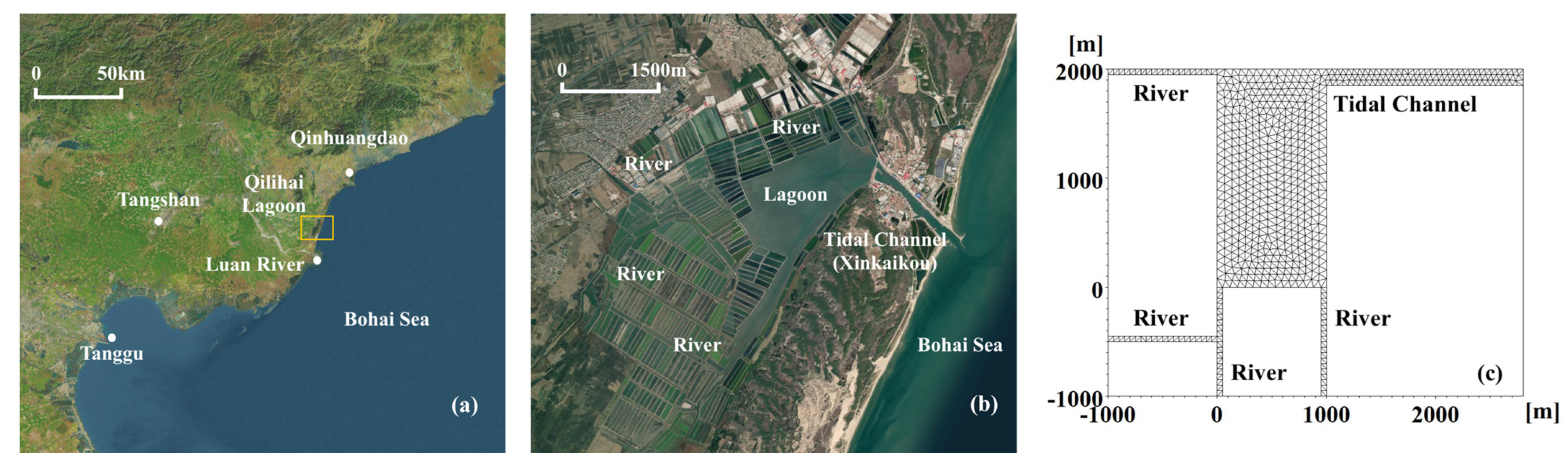
2.1. Selection of a Typical Tidal Lagoon
2.2. The Ideal Model
2.3. Model Set Up
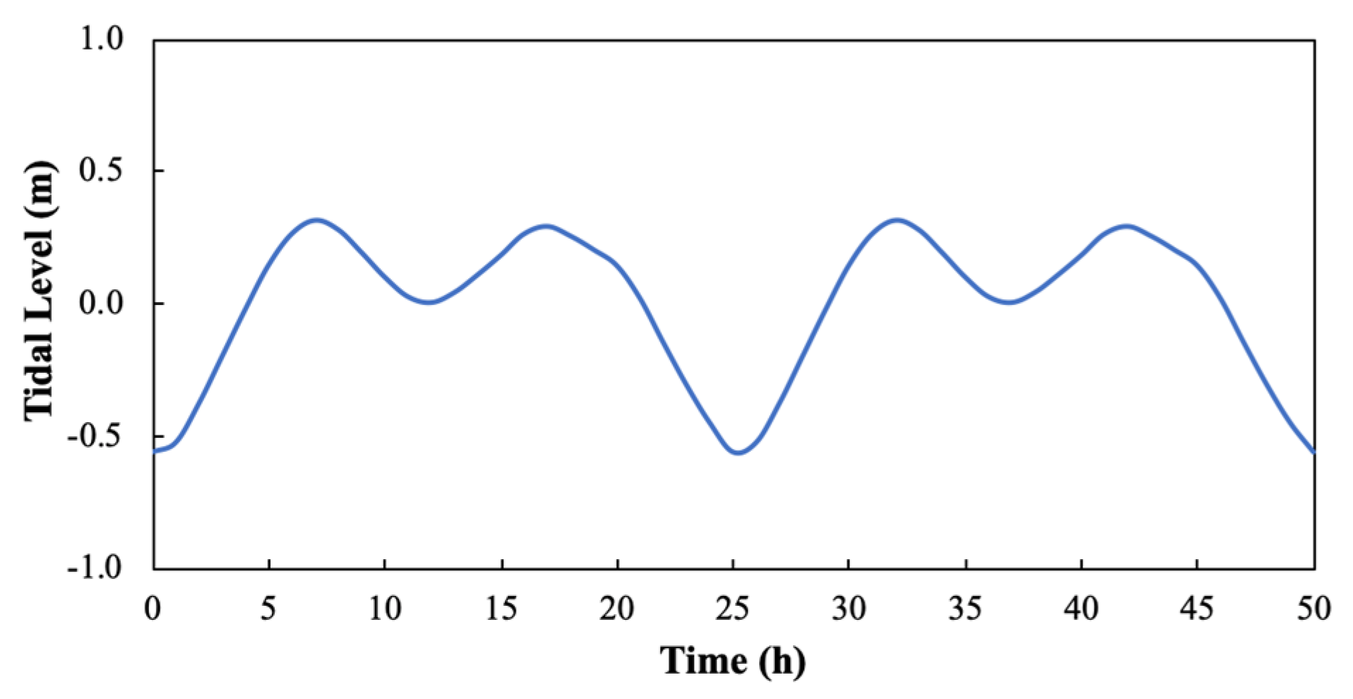
2.3.1. Control Group
2.3.2. Sediment Transport
2.4. Variable Importance Analysis
3. Model Results and Analysis
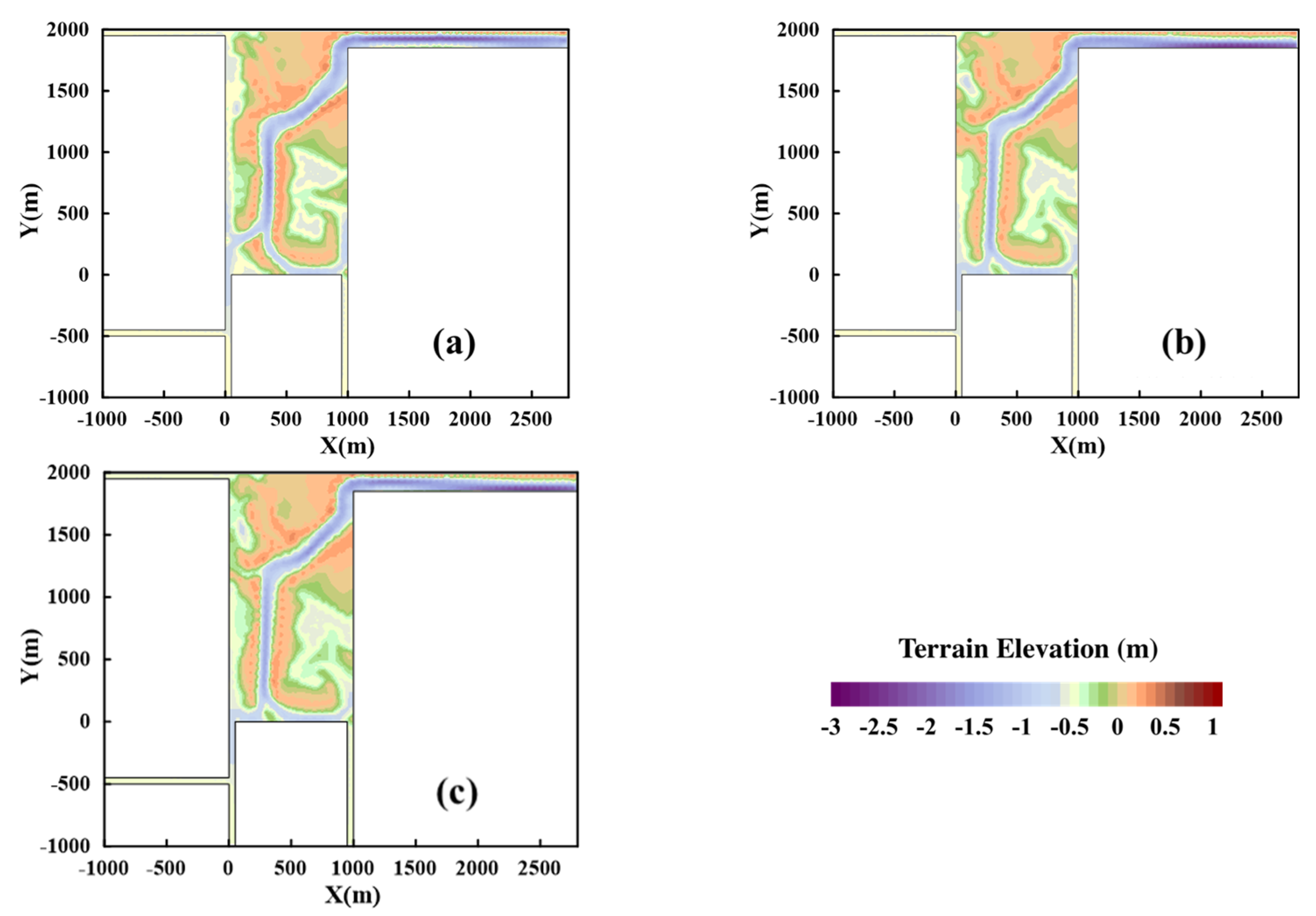
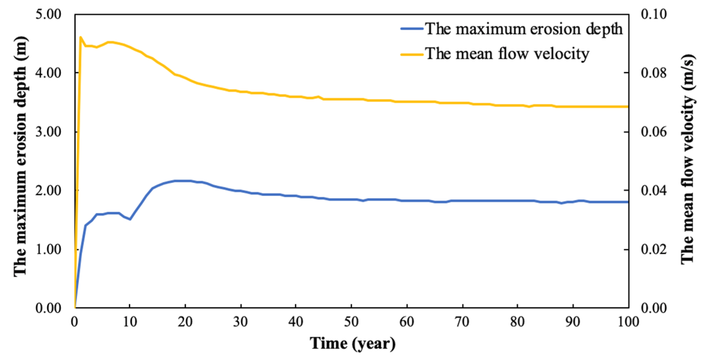
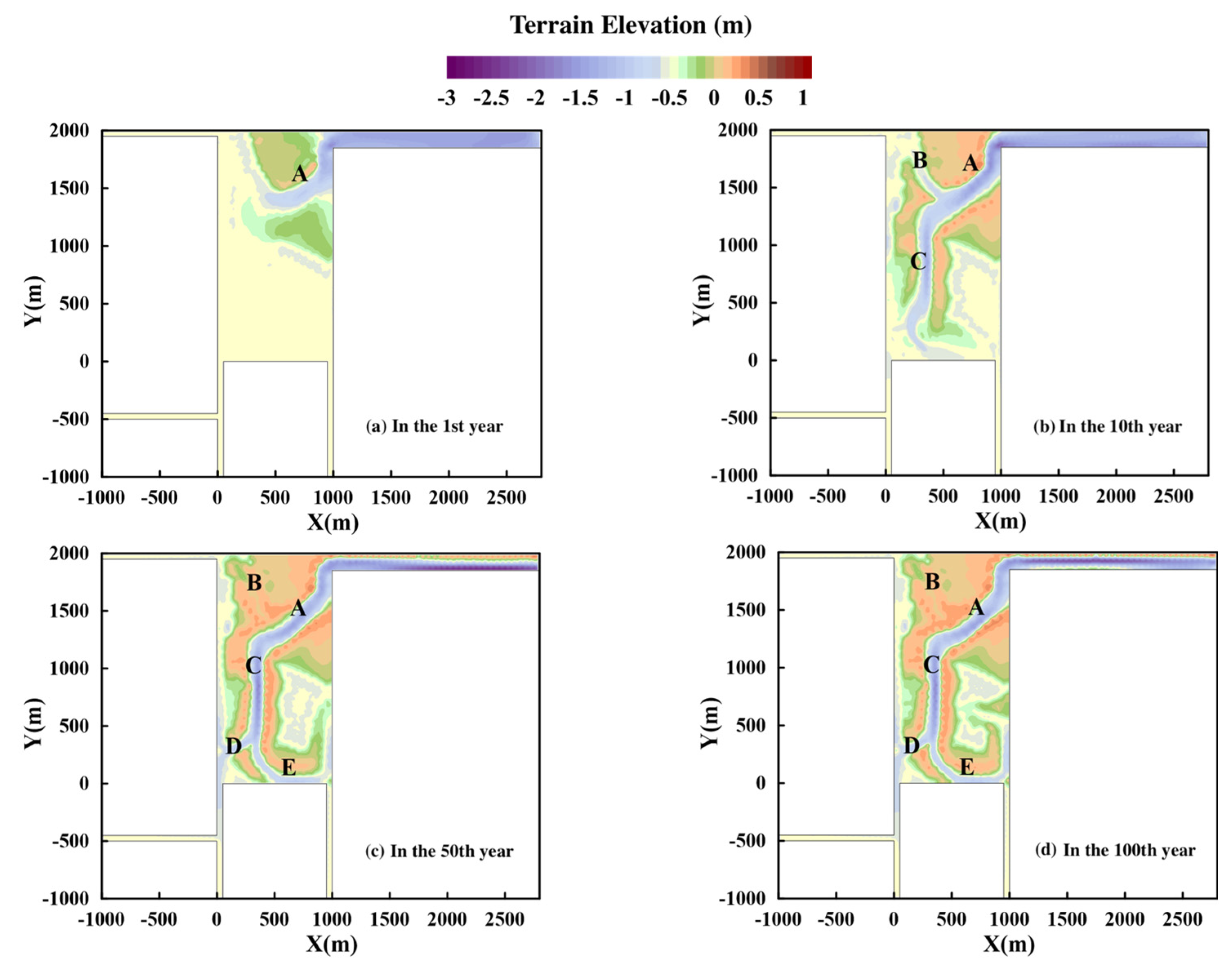
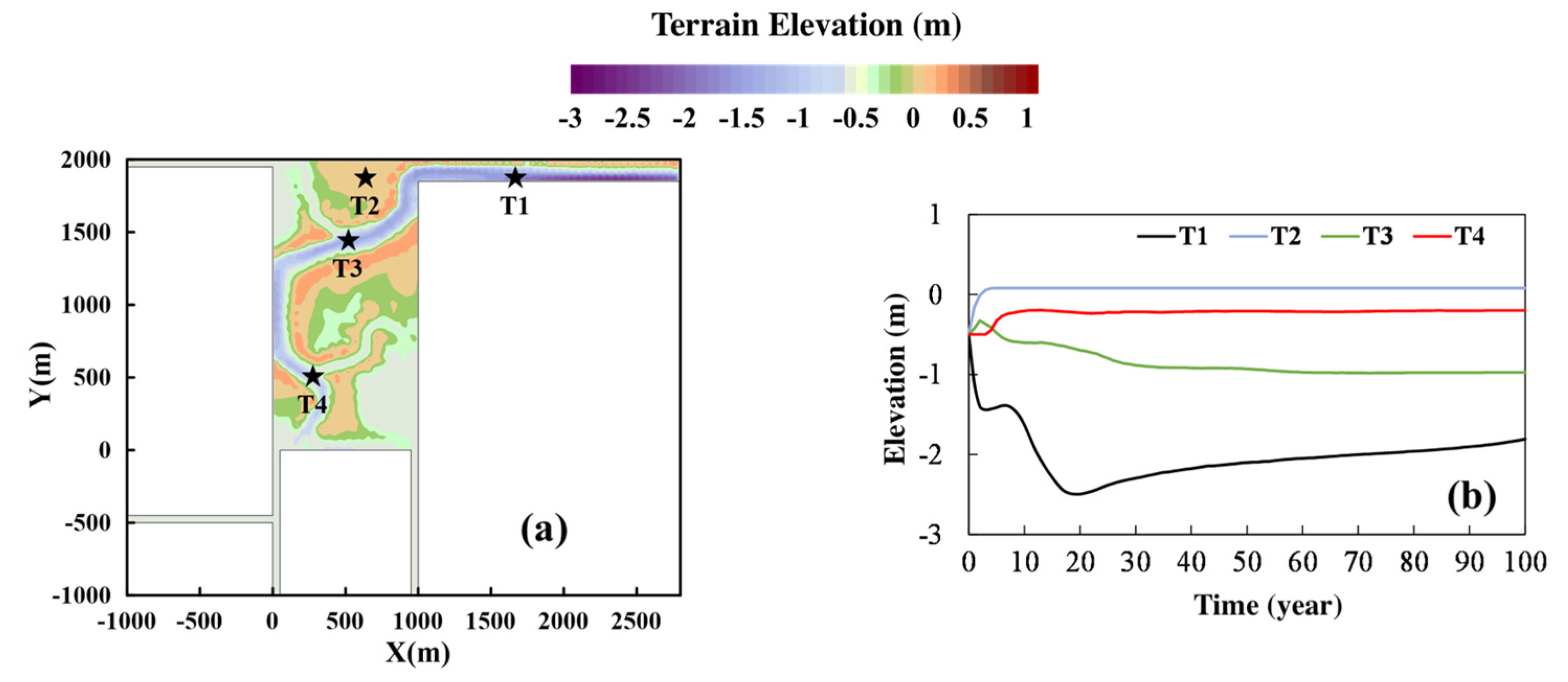
3.1. Control Group
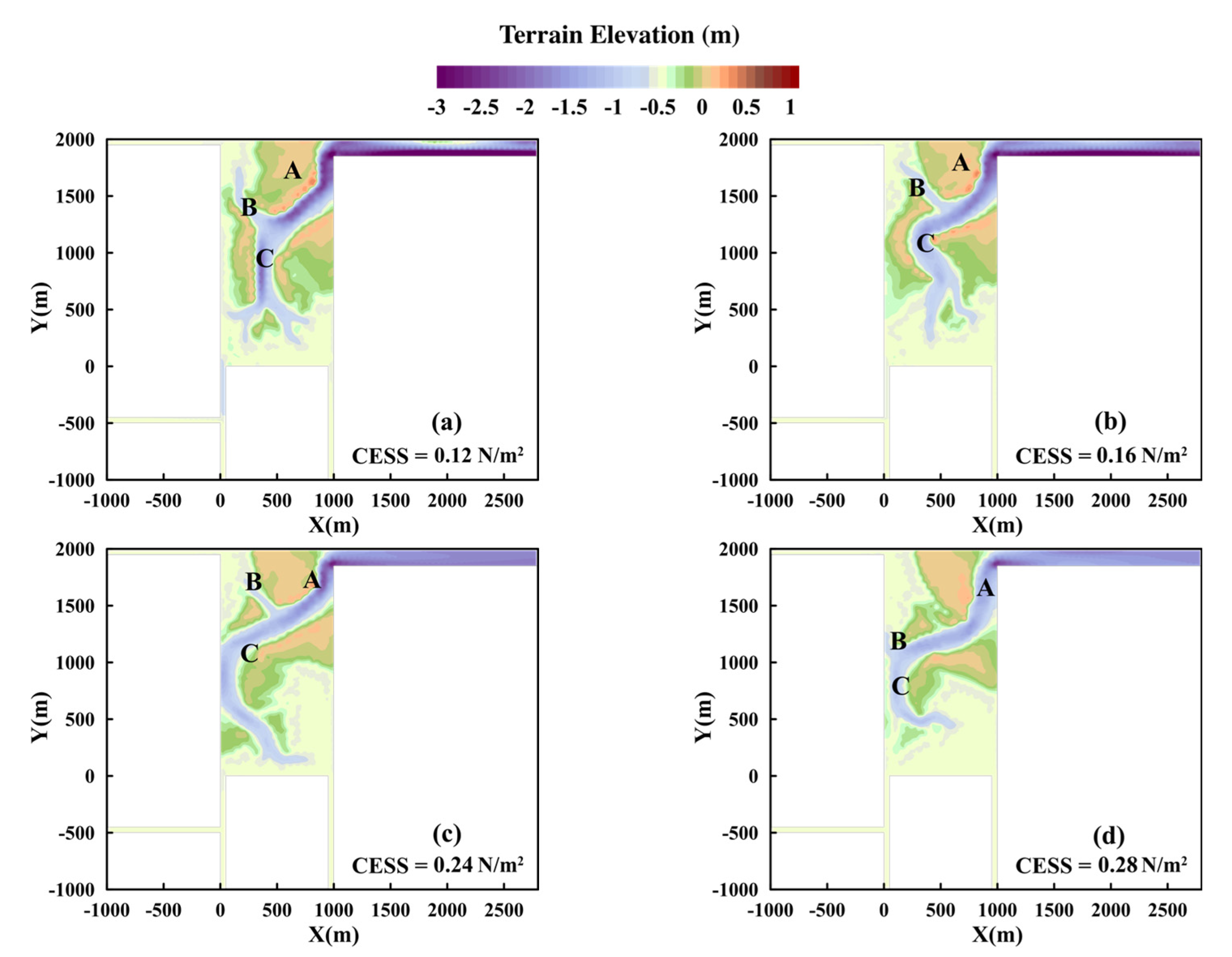
3.2. Impacts of CESS
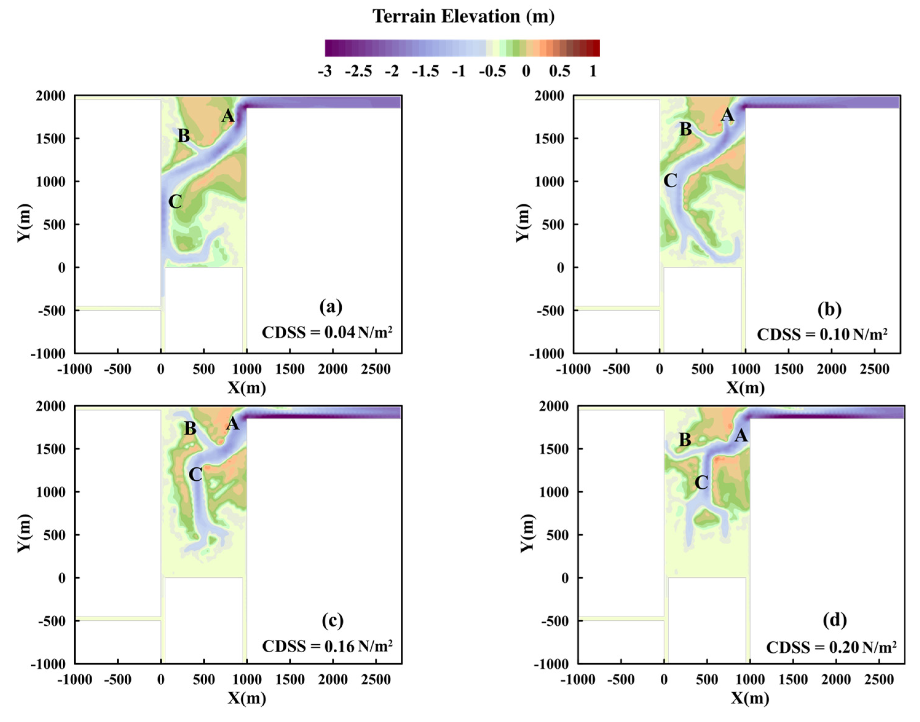
3.3. Impacts of CDSS
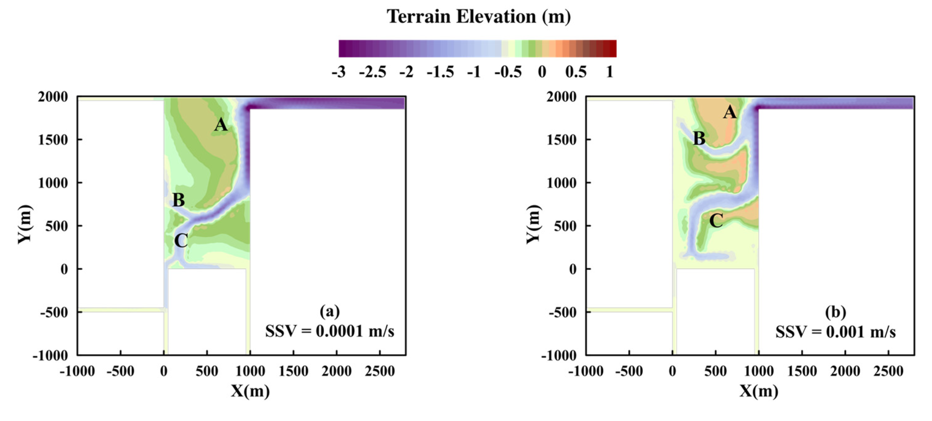
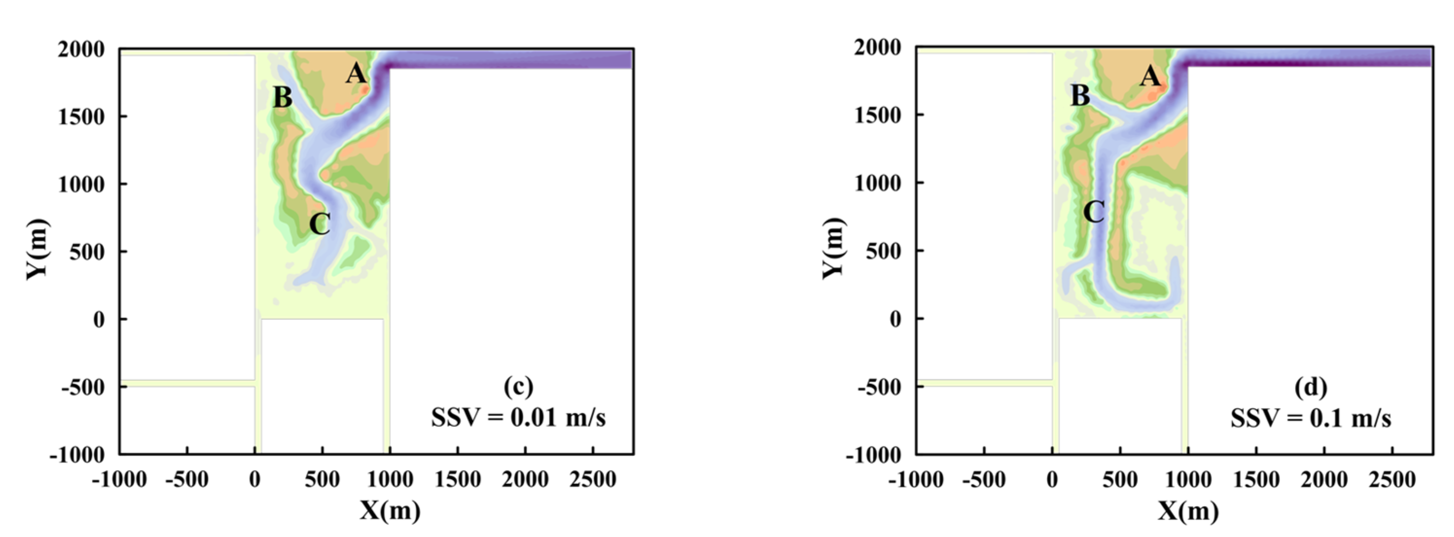
3.4. Impacts of SSV
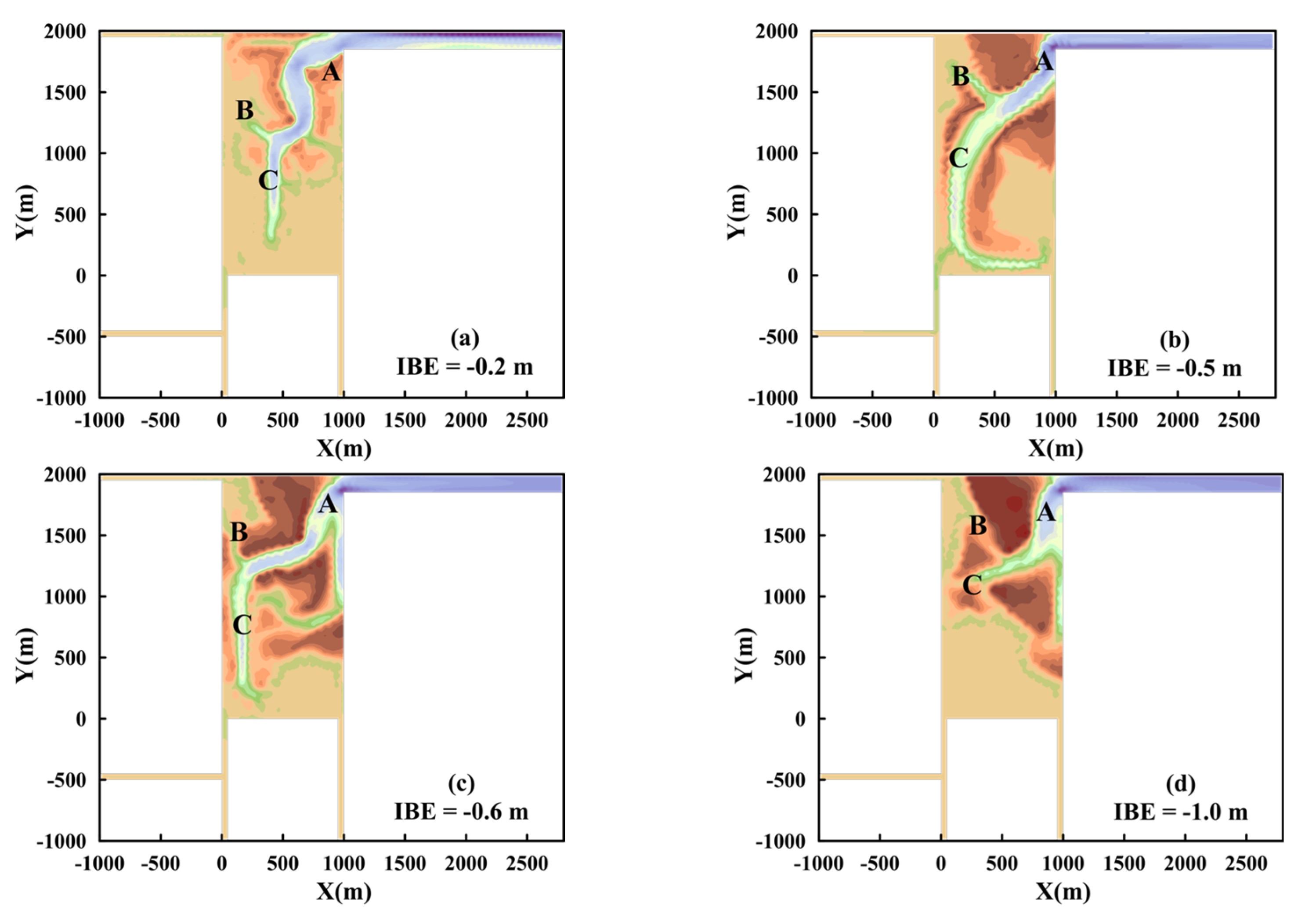
3.5. Impacts of IBE
4. Discussions
4.1. Reliability of Model Results
4.2. Variable Importance Analysis
4.3. Influences of SLR
5. Conclusions
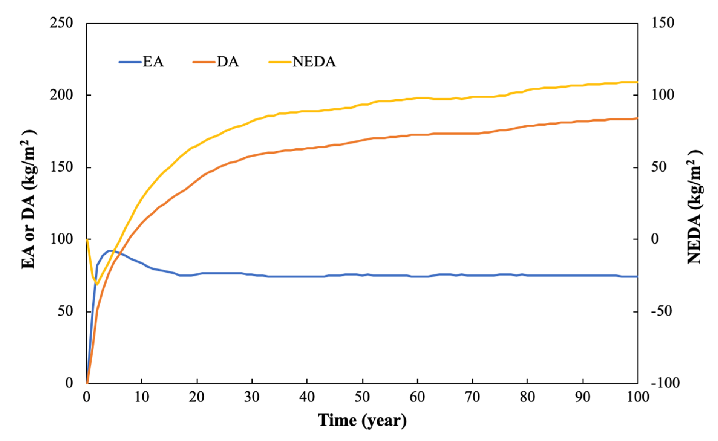
- The lagoon geomorphological evolution is active in the tidal channel, but hysteretic in the lagoon. The generation of tidal networks promotes the evolution towards reaching an equilibrium state. An increase of CESS, CDSS, SSV, or water depth (due to the descent of IBE) has a beneficial effect on the evolution.
- The erosion effect and the deposition effect counteract each other, so that the lagoon terrain eventually attains the equilibrium state when the change of net erosion amount per unit area remains within .
- The influence by the IBE mainly depends on the lowest tidal level. If the IBE is below the lowest tidal level, the deposition effect is more sensitive to the variation of IBE. However, if the IBE is above the lowest tidal level, the variation of IBE causes more erosion.
- According to the variable importance analysis, EA is highly correlated with other variables. In addition, CESS and CDSS showed a more direct effect on the geomorphological evolution than SSV and IBE. Thus, it is more effective to alter the evolution by changing CESS or CDSS.
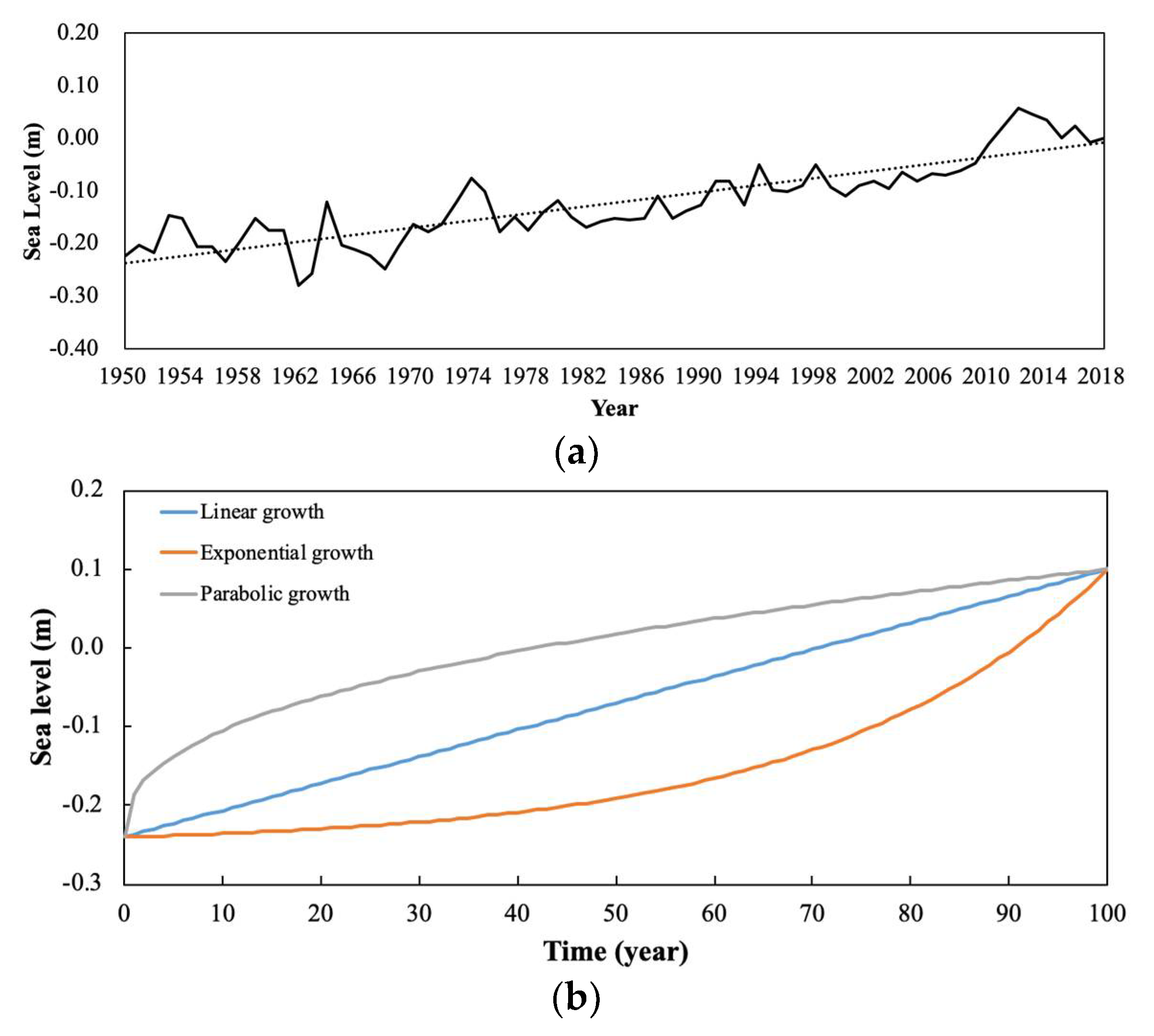
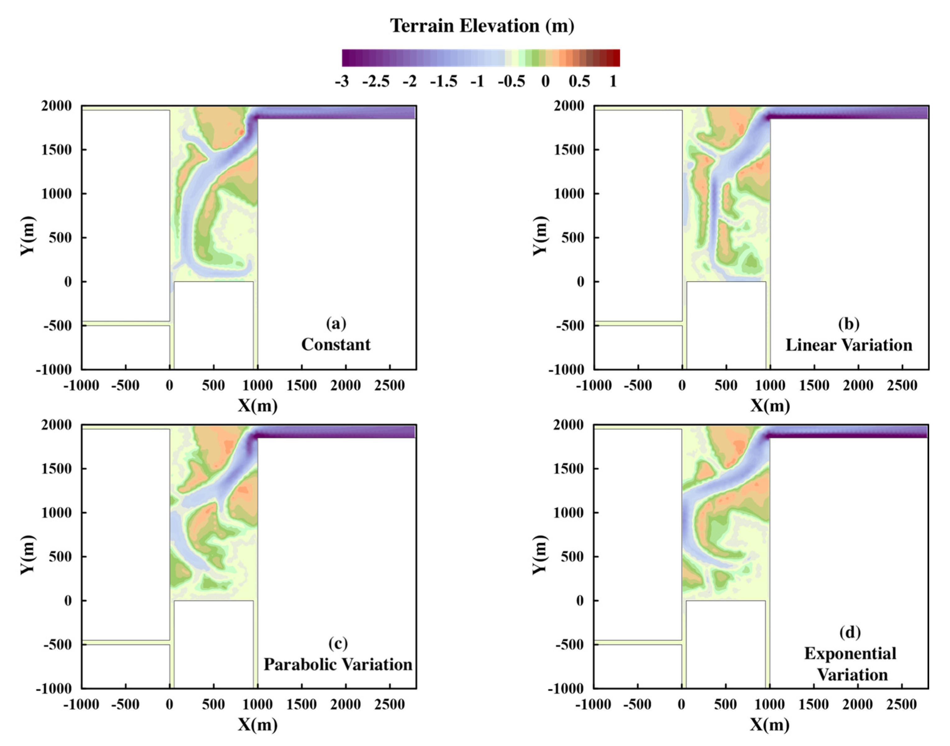
- SLR is considered the only external contributing factor for lagoon evolution that can be estimated reasonably well. This indicates that an exponential variation of SLR would give rise to more intensive erosion in a lagoon in the long-term compared with linear variation and parabolic variation of SLR.
Author Contributions
Funding
Institutional Review Board Statement
Informed Consent Statement
Data Availability Statement
Acknowledgments
Conflicts of Interest
References
- Duong, T.M.; Ranasinghe, R.; Walstra, D.; Roelvink, D. Assessing climate change impacts on the stability of small tidal inlet systems: Why and how? Earth-Sci. Rev. 2016, 154, 369–380. [Google Scholar] [CrossRef]
- Jeanson, M.; Dolique, F.; Anthony, E.J.; Aubry, A. Decadal-scale dynamics and morphological evolution of mangroves and beaches in a reef-lagoon complex, mayotte island. J. Coast. Res. 2019, 88, 195–208. [Google Scholar] [CrossRef]
- Drost, E.; Cuttler, M.; Lowe, R.J.; Hansen, J.E. Predicting the hydrodynamic response of a coastal reef-lagoon system to a tropical cyclone using phase-averaged and surfbeat-resolving wave models. Coast. Eng. 2019, 152, 103525. [Google Scholar] [CrossRef]
- Wang, Q.; Su, F.Z.; Zhang, Y.; Jiang, H.P.; Cheng, F. Morphological precision assessment of reconstructed surface models for a coral atoll lagoon. Sustainability 2018, 10, 2749. [Google Scholar] [CrossRef]
- Sun, W.F.; Zhang, J.; Ma, Y.; Xia, D.X. Investigation of the evolution of China coastal lagoons from 1979 to 2010 using multi-temporal satellite data. Acta Oceanol. Sin. 2015, 37, 54–69. [Google Scholar]
- Costanza, R.; Farber, S.C.; Maxwell, J. Valuation and management of wetland ecosystems. Ecol. Econ. 1989, 1, 335–361. [Google Scholar] [CrossRef]
- Barbier, E.B.; Hacker, S.D.; Kennedy, C.; Koch, C.; Stier, A.C.; Silliman, B.R. The value of estuarine and coastal ecosystem services. Ecol. Monogr. 2011, 81, 169–193. [Google Scholar] [CrossRef]
- Zhou, Z.; Chen, L.Y.; Tao, J.F.; Gong, Z.; Guo, L.C.; Wegen, M.; Townend, I.; Zhang, C.K. The role of salinity in fluvio-deltaic morphodynamics: A long-term modelling study. Earth Surf. Processes Landf. 2020, 45, 590–604. [Google Scholar] [CrossRef]
- Carrasco, A.R.; Plomaritis, T.; Reyns, J.; Ferreira, O.; Roelvink, D. Tide circulation patterns in a coastal lagoon under sea-level rise. Ocean Dyn. 2018, 68, 1–19. [Google Scholar] [CrossRef]
- Madricardo, F.; Foglini, F.; Campiani, E.; Grande, V.; Catenacci, E.; Petrizzo, A. Assessing the human footprint on the sea-floor of coastal systems: The case of the Venice Lagoon, Italy. Sci. Rep. 2019, 9, 1–13. [Google Scholar]
- Roversi, F.; Maanen, B.V.; Rosman, P.; Neves, C.F.; Scudelari, A.C. Numerical modeling evaluation of the impacts of shrimp farming operations on long-term coastal lagoon morphodynamics. Estuaries Coasts 2020, 43, 1853–1872. [Google Scholar] [CrossRef]
- Masters, P.M.; Aiello, I.W. Postglacial evolution of coastal environments. In California Prehistory: Colonization, Culture, and Complexity; Rowman Altamira: Lanham, MA, USA, 2007; pp. 35–51. [Google Scholar]
- Lewis, S.E.; Sloss, C.R.; Murray-Wallace, C.V.; Woodroffe, C.D.; Smithers, S.G. Post-glacial sea-level changes around the australian margin: A review. Quat. Sci. Rev. 2013, 74, 115–138. [Google Scholar] [CrossRef]
- Bortolin, E.; Weschenfelder, J.; Cooper, A. Holocene evolution of Patos lagoon, Brazil: The role of antecedent topography. J. Coast. Res. 2019, 35, 357–368. [Google Scholar] [CrossRef]
- Petti, M.; Bosa, S.; Pascolo, S.; Ulina, E. An integrated approach to study the morphodynamics of the Lignano tidal inlet. J. Mar. Sci. Eng. 2020, 8, 77. [Google Scholar] [CrossRef]
- Petti, M.; Bosa, S.; Pascolo, S.; Ulina, E. Marano and Grado Lagoon: Narrowing of the Lignano Inlet; IOP Conference Series: Materials Science and Engineering; IOP Publishing: Bristol, UK, 2019; p. 32066. [Google Scholar]
- Roelvink, J.; Walstra, D.; Chen, Z. Morphological modelling of Keta lagoon case. In Proceedings of the 24th International Conference on Coastal Engineering, Kobe, Japan, 23–28 October 1994; American Society of Civil Engineers: Reston, VA, USA, 1995; pp. 3223–3236. [Google Scholar]
- Tambroni, N.; Pittaluga, M.B.; Seminara, G. Laboratory observations of the morphodynamic evolution of tidal channels and tidal inlets. J. Geophys. Res. Earth Surf. 2005, 110, F4009. [Google Scholar] [CrossRef]
- Fitzgerald, D.M. Response characteristics of an ebb-dominated tidal inlet channel. J. Sediment. Res. 1983, 53, 833–845. [Google Scholar]
- Cayocca, F. Long-term morphological modeling of a tidal inlet: The Arcachon Basin, France. Coast. Eng. 2001, 42, 115–142. [Google Scholar] [CrossRef]
- Lam, N.T.; Stive, M.J.; Wang, Z.B. Hydrodynamics and morphodynamics of a seasonally forced tidal inlet system. J. Water Resour. Environ. Eng. 2008, 23, 114–124. [Google Scholar]
- Hume, T.M.; Snelder, T.; Weatherhead, M.; Leifting, R. A controlling factor approach to estuary classification. Ocean Coast. Manag. 2007, 50, 905–929. [Google Scholar] [CrossRef]
- Whitehouse, R.; Bassoullet, P.; Dyer, K.R.; Mitchener, H.J.; Roberts, W. The influence of bedforms on flow and sediment transport over intertidal mudflats. Cont. Shelf Res. 2000, 20, 1099–1124. [Google Scholar] [CrossRef]
- Andrew, M.; Collins, M. The establishment and degeneration of a temporary creek system in response to managed coastal realignment: The Wash, UK. Earth Surf. Processes Landf. 2007, 32, 1783–1796. [Google Scholar]
- Coco, G.; Zhou, Z.; Maanen, B.V.; Olabarrieta, M.; Tinoco, R.; Townend, I. Morphodynamics of tidal networks: Advances and challenges. Mar. Geol. 2013, 346, 1–16. [Google Scholar] [CrossRef]
- Vriend, H.; Capobianco, M.; Chesher, T.; Swart, H.; Latteux, B.; Stive, M. Approaches to long-term modelling of coastal morphology: A review. Coast. Eng. 1993, 21, 225–269. [Google Scholar] [CrossRef]
- Marani, M.; D’Alpaos, A.; Lanzoni, S.; Carniello, L.; Rinaldo, A. The importance of being coupled: Stable states and catastrophic shifts in tidal biomorphodynamics. J. Geophys. Res. Earth Surf. 2010, 115, F4004. [Google Scholar] [CrossRef]
- Stefanon, L.; Carniello, L.; D’Alpaos, A.; Lanzoni, S. Experimental analysis of tidal network growth and development. Cont. Shelf Res. 2010, 30, 950–962. [Google Scholar] [CrossRef][Green Version]
- Reynolds, O. Report of the Committee Appointed to Investigate the Action of Waves and Currents on the Beds and Foreshores of Estuaries by Means of Working Models. British Association Report. Mech. Phys. Subj. 1889, 2, 1881–1900. [Google Scholar]
- Reynolds, O. Second Report of the Committee Appointed to Investigate the Action of Waves and Currents on the Beds and Foreshores of Estuaries by Means of Working Models; Spottiswoode and Company: London, UK, 1891. [Google Scholar]
- Reynolds, O. Third Report of the Committee Appointed to Investigate the Action of Waves and Currents on the Beds and Foreshores of Estuaries by Means of Working Models; Spottiswoode and Company: London, UK, 1892. [Google Scholar]
- Deigaard, R.; Fredsoe, J. Mechanics of Coastal Sediment Transport; World Scientific Publishing Company: Singapore, 1992. [Google Scholar]
- Nielsen, P. Coastal Bottom Boundary Layers and Sediment Transport; World Scientific: Singapore, 1992. [Google Scholar]
- Rijn, L.C. Principles of Sediment Transport in Rivers, Estuaries and Coastal Seas; Aqua Publications: Amsterdam, The Netherlands, 1993. [Google Scholar]
- Soulsby, R. Dynamics of marine sands: A manual for practical applications. Oceanogr. Lit. Rev. 1997, 9, 947. [Google Scholar]
- Li, L.; Guan, W.B.; He, Z.G.; Yao, Y.M.; Xia, Y.Z. Responses of water environment to tidal flat reduction in Xiangshan bay: Part II locally re-suspended sediment dynamics. Estuarine, Coast. Shelf Sci. 2017, 198, 114–127. [Google Scholar] [CrossRef]
- Kleinhans, M.G.; Vegt, M.; Scheltinga, R.; Baar, A.W.; Markies, H. Turning the tide: Experimental creation of tidal channel networks and ebb deltas. Neth. J. Geosci. 2012, 91, 311–323. [Google Scholar] [CrossRef]
- Amos, C.L.; Kassem, H.; Bergamasco, A.; Sutherland, T.F.; Cloutier, D. The mass settling flux of suspended particulate matter in Venice Lagoon, Italy. J. Coast. Res. 2021, 37, 1099–1116. [Google Scholar] [CrossRef]
- Marciano, R.; Wang, Z.B.; Hibma, A.; de Vriend, H.J.; Defina, A. Modeling of channel patterns in short tidal basins. J. Geophys. Res. Earth Surf. 2005, 110, F1001. [Google Scholar] [CrossRef]
- Roelvink, J.A. Coastal morphodynamic evolution techniques. Coast. Eng. 2006, 53, 277–287. [Google Scholar] [CrossRef]
- Vlaswinkel, B.M.; Cantelli, A. Geometric characteristics and evolution of a tidal channel network in experimental setting. Earth Surf. Processes Landf. 2011, 36, 739–752. [Google Scholar] [CrossRef]
- Iwasaki, T.; Shimizu, Y.; Kimura, I. Modelling of the initiation and development of tidal creek networks. In Proceedings of the Institution of Civil Engineers-Maritime Engineering; Thomas Telford Ltd.: London, UK, 2013. [Google Scholar]
- Stefan, A.T.; David, A.J. Changing Tides: The Role of Natural and Anthropogenic Factors. Annu. Rev. Mar. Sci. 2020, 12, 121–151. [Google Scholar]
- Yin, Y.Z.; Karunarathna, H.; Reeve, D.E. Numerical modelling of hydrodynamic and morphodynamic response of a meso-tidal estuary inlet to the impacts of global climate variabilities. Mar. Geol. 2019, 407, 229–247. [Google Scholar] [CrossRef]
- Szydłowski, M.; Artichowicz, W.; Zima, P. Analysis of the water level variation in the polish part of the Vistula Lagoon (Baltic Sea) and estimation of water inflow and outflow transport through the Strait of Baltiysk in the Years 2008–2017. Water 2021, 13, 1328. [Google Scholar] [CrossRef]
- Lopes, J.F.; Lopes, C.L.; Dias, J.M. Extreme Meteorological Events in a Coastal Lagoon Ecosystem: The Ria de Aveiro Lagoon (Portugal) Case Study. J. Mar. Sci. Eng. 2021, 9, 727. [Google Scholar] [CrossRef]
- Shalby, A.; Elshemy, M.; Zeidan, B.A. Modeling of climate change impacts on Lake Burullus, coastal lagoon (Egypt). Int. J. Sediment. Res. 2021, 36, 756–769. [Google Scholar] [CrossRef]
- Bruneau, N.; Fortunato, A.B.; Dodet, G.; Dodet, G.; Freire, P. Future evolution of a tidal inlet due to changes in wave climate, Sea level and lagoon morphology (bidos lagoon, Portugal). Cont. Shelf Res. 2011, 31, 1915–1930. [Google Scholar] [CrossRef]
- Lodder, Q.J.; Wang, Z.B.; Elias, E.; Spek, A.; Looff, H.; Townend, I. Future response of the Wadden Sea tidal basins to relative sea-level rise—An aggregated modelling approach. Water 2019, 11, 2198. [Google Scholar] [CrossRef]
- Parker, A.; Saleem, M.S.; Lawson, M. Sea-level trend analysis for coastal management. Ocean Coast. Manag. 2013, 73, 63–81. [Google Scholar] [CrossRef]
- Sun, W.F. Monitoring and Analyzing the Lagoon Dynamics in China Using Remote Sensing Imagery. Ph.D. Dissertation, Ocean University of China, Qingdao, China, 2013. [Google Scholar]
- Xing, R.R.; Liu, X.J.; Qiu, R.F. Recent evolution analysis and ecological restoration of Qilihai Lagoon wetland. Ocean. Dev. Manag. 2019, 36, 64–68. [Google Scholar]
- Yuan, Z.; Yang, H.; Gao, W. The evolution and restoration of Qilihai Lagoon. Ocean. Dev. Manag. 2008, 6, 98–103. [Google Scholar]
- Bokulich, A. Models and Explanation; Springer Handbook of Model-Based Science; Springer: Berlin/Heidelberg, Germany, 2017; pp. 103–118. [Google Scholar]
- Cong, X.; Kuang, C.P.; Dong, Z.C.; Gong, L.X.; Liu, H.X.; Zhu, L. Responses of Morphological Stability to Tidal Inlet width of a Shallow Coastal Lagoon. In The Fourteenth ISOPE Pacific/Asia Offshore Mechanics Symposium; International Society of Offshore and Polar Engineers: Dalian, China, 2020. [Google Scholar]
- Kuang, C.P.; Dong, Z.C.; Gu, J.; Su, T.C.; Zhan, H.M.; Zhao, W. Quantifying the influence factors on water exchange capacity in a shallow coastal lagoon. J. Hydro-Environ. Res. 2020, 31, 26–40. [Google Scholar] [CrossRef]
- MIKE Powered by DHI. Available online: https://www.mikepoweredbydhi.com (accessed on 9 December 2021).
- Kuang, C.; Cong, X.; Dong, Z.; Zou, Q.; Zhan, H.; Zhao, W. Impact of anthropogenic activities and sea level rise on a lagoon system: Model and field observations. J. Mar. Sci. Eng. 2021, 9, 1393. [Google Scholar] [CrossRef]
- Ren, H.R.; Li, G.S.; Guo, T.J.; Zhang, Y.; Ouyang, N.L. Multi-scale Variability of Surface Wind Direction and Speed on the Bohai Sea in 1950-2011. Sci. Geogr. Sin. 2017, 37, 1430–1438. [Google Scholar]
- Partheniades, E. Erosion and deposition of cohesive soils. J. Hydraul. Div. 1965, 91, 105–139. [Google Scholar] [CrossRef]
- Krone, R.B. Flume Study of the Transport of Sediment in Estuarial Processes; Hydraulic Engineering Laboratory and Sanitary Engineering Research Laboratory, University of California: Oakland, CA, Canada, 1962. [Google Scholar]
- Wang, Y.P.; Voulgaris, G.; Li, Y.; Yang, Y.; Gao, J.H.; Chen, J.; Gao, S. Sediment resuspension, flocculation, and settling in a macrotidal estuary. J. Geophys. Res. Oceans. 2013, 118, 5591–5608. [Google Scholar] [CrossRef]
- Cheng, N. Simplified settling velocity formula for sediment particle. J. Hydraul. Eng. 1997, 123, 149–152. [Google Scholar] [CrossRef]
- Benesty, J.; Chen, J.; Huang, Y. Pearson Correlation Coefficient. Noise Reduction in Speech Processing; Springer: Berlin/Heidelberg, Germany, 2009. [Google Scholar]
- Dong, Z.C.; Kuang, C.P.; Gu, J.; Zou, Q.P.; Zhang, J.B.; Liu, H.X.; Zhu, L. Total maximum allocated load of chemical oxygen demand near Qinhuangdao in Bohai sea: Model and field observations. Water 2020, 12, 1141. [Google Scholar] [CrossRef]
- Kotz, S.; Read, C.B.; Balakrishnan, N.; Vidakovic, B.; Johnson, N.L. Spearman correlation coefficients, differences between. Encycl. Stat. Sci. 2004, 12, 1–2. [Google Scholar] [CrossRef]
- Zhou, Z.; Coco, G.; Townend, I.; Olabarrieta, M.; Mick, V.; Gong, Z.; D’Alpos, A.; Jaffe, B.; Gelfenbaum, G. Is “morphodynamic equilibrium” an oxymoron? Earth-Sci. Rev. 2017, 165, 257–267. [Google Scholar] [CrossRef]
- Lanzoni, S.; Seminara, G. Long-term evolution and morphodynamic equilibrium of tidal channels. J. Geophys. Res. 2002, 107, 3001. [Google Scholar] [CrossRef]
- Ward, R.D. Sedimentary response of Arctic coastal wetlands to sea level rise. Geomorphology 2020, 370, 107400. [Google Scholar] [CrossRef]


| Dependent Variables | CESS (N/m2) | ||||||||||
|---|---|---|---|---|---|---|---|---|---|---|---|
| 0.10 | 0.12 | 0.14 | 0.16 | 0.18 | 0.20 | 0.22 | 0.24 | 0.26 | 0.28 | 0.30 | |
| EA (kg/m2) | 197.1 | 183.3 | 167.9 | 159.6 | 151.2 | 144.0 | 138.7 | 130.8 | 120.2 | 114.6 | 111.1 |
| DA (kg/m2) | 101.8 | 100.8 | 95.3 | 92.2 | 90.0 | 89.3 | 87.3 | 84.7 | 78.7 | 76.1 | 74.8 |
| NEA (kg/m2) | 95.3 | 82.5 | 72.6 | 67.4 | 61.2 | 54.7 | 51.3 | 46.1 | 41.5 | 38.5 | 36.3 |
| Dependent Variables | CDSS (N/m2) | |||||||||
|---|---|---|---|---|---|---|---|---|---|---|
| 0.02 | 0.04 | 0.06 | 0.08 | 0.10 | 0.12 | 0.14 | 0.16 | 0.18 | 0.20 | |
| EA (kg/m2) | 149.5 | 148.2 | 145.9 | 144.7 | 142.1 | 140.7 | 134.9 | 129.0 | 123.8 | 118.9 |
| DA (kg/m2) | 94.0 | 92.7 | 91.0 | 89.9 | 88.8 | 87.7 | 83.3 | 80.3 | 78.0 | 76.8 |
| NEA (kg/m2) | 55.5 | 55.6 | 54.9 | 54.9 | 53.4 | 52.9 | 51.6 | 48.7 | 45.8 | 42.1 |
| Dependent Variables | SSV (m/s) | ||||||
|---|---|---|---|---|---|---|---|
| 0.0001 | 0.0005 | 0.001 | 0.005 | 0.01 | 0.05 | 0.1 | |
| EA (kg/m2) | 179.0 | 159.1 | 153.0 | 149.2 | 141.3 | 139.6 | 138.5 |
| DA (kg/m2) | 109.7 | 98.0 | 94.4 | 94.3 | 86.8 | 86.0 | 85.7 |
| NEA (kg/m2) | 69.4 | 61.1 | 58.6 | 54.9 | 54.5 | 53.6 | 52.8 |
| Dependent Variables | IBE (m) | |||||||||
|---|---|---|---|---|---|---|---|---|---|---|
| −0.1 | −0.2 | −0.3 | −0.4 | −0.5 | −0.6 | −0.7 | −0.8 | −0.9 | −1.0 | |
| EA (kg/m2) | 120.4 | 127.3 | 133.2 | 137.2 | 144.0 | 130.9 | 123.2 | 113.9 | 105.6 | 98.4 |
| DA (kg/m2) | 15.2 | 29.3 | 50.2 | 70.7 | 89.3 | 85.5 | 82.3 | 77.1 | 72.1 | 68.0 |
| NEA (kg/m2) | 105.2 | 98.0 | 83.0 | 66.6 | 54.7 | 45.4 | 40.9 | 36.8 | 33.5 | 30.3 |
| Dependent Variables | Independent Variables | Dependent Variables | |||||
|---|---|---|---|---|---|---|---|
| CESS | CDSS | SSV | IBE | EA | DA | NEA | |
| EA | 0.613 | 0.533 | 0.291 | 0.110 | 0.928 | 0.724 | |
| DA | 0.479 | 0.526 | 0.352 | 0.024 | 0.928 | 0.455 | |
| NEA | 0.590 | 0.357 | 0.228 | 0.625 | 0.724 | 0.455 | |
| Average | 0.561 | 0.472 | 0.290 | 0.253 | 0.826 | 0.692 | 0.590 |
| Dependent Variables | Sea Level Rise Scenarios | |||
|---|---|---|---|---|
| Constant | Exponential Variation | Linear Variation | Parabolic Variation | |
| EA (kg/m2) | 145.01 | 151.37 | 149.27 | 148.85 |
| DA (kg/m2) | 90.30 | 97.72 | 99.54 | 103.29 |
| NEA (kg/m2) | 54.71 | 53.65 | 49.73 | 45.56 |
Publisher’s Note: MDPI stays neutral with regard to jurisdictional claims in published maps and institutional affiliations. |
© 2022 by the authors. Licensee MDPI, Basel, Switzerland. This article is an open access article distributed under the terms and conditions of the Creative Commons Attribution (CC BY) license (https://creativecommons.org/licenses/by/4.0/).
Share and Cite
Kuang, C.; Fan, J.; Dong, Z.; Zou, Q.; Cong, X.; Han, X. Influence Mechanism of Geomorphological Evolution in a Tidal Lagoon with Rising Sea Level. J. Mar. Sci. Eng. 2022, 10, 108. https://doi.org/10.3390/jmse10010108
Kuang C, Fan J, Dong Z, Zou Q, Cong X, Han X. Influence Mechanism of Geomorphological Evolution in a Tidal Lagoon with Rising Sea Level. Journal of Marine Science and Engineering. 2022; 10(1):108. https://doi.org/10.3390/jmse10010108
Chicago/Turabian StyleKuang, Cuiping, Jiadong Fan, Zhichao Dong, Qingping Zou, Xin Cong, and Xuejian Han. 2022. "Influence Mechanism of Geomorphological Evolution in a Tidal Lagoon with Rising Sea Level" Journal of Marine Science and Engineering 10, no. 1: 108. https://doi.org/10.3390/jmse10010108
APA StyleKuang, C., Fan, J., Dong, Z., Zou, Q., Cong, X., & Han, X. (2022). Influence Mechanism of Geomorphological Evolution in a Tidal Lagoon with Rising Sea Level. Journal of Marine Science and Engineering, 10(1), 108. https://doi.org/10.3390/jmse10010108