1. Introduction
International competition can potentially lead governments to disregard natural resource conservation and engage in a regulatory race to the bottom designed to increase competitiveness. If the government is industry-biased and weighs industry income more heavily than consumption and conservation benefits, it may be even more willing to sacrifice the environment [
1]. According to Peterson and Bielke [
2], for example, “A decree by Russian President Vladimir Putin in May 2000 abolished the Russian Federation State Committee for Environmental Protection and shifted its personnel and responsibilities for environmental protection to the Russian Federation Ministry of Natural Resources…Putin also rolled over the duties of the 200-year-old Federal Forestry Service (Goskomles)…(which) was responsible for regulating logging, for forest health monitoring, and for fire protection...(The) probable goals of the Russian leadership in abolishing Goskomekologiya (State Committee for the Protection of the Natural Environment) were to reduce environmental regulation of industry, encourage natural resource development, and attract foreign investors to the natural resources sector… Putin’s support for energy and natural resource development likely is the result of pressure from the country’s powerful corporate interests, particularly in the energy sector”.
In this paper, we ask how the presence of industry-biased as opposed to welfare-maximizing governments changes the environmental impact of international trade liberalization. We address the question using a two-country model of trade under imperfect competition. The model combines the Brander and Krugman [
3] “reciprocal dumping” model of trade, where firms export identical products to capture market share abroad, the Brander and Spencer [
4] model, which adds a pre-trade policymaking stage, and the assumption that the policymakers are industry biased. We model the industry bias (e.g., [
5,
6,
7]) by assuming that the government’s objective function weighs industry income more heavily than consumer surplus and utility from forest conservation.
We believe that the model’s assumptions are empirically relevant. For example, current history shows a number of examples of trade liberalization between homogenous neighboring countries. Countries of Central Asia discuss the development of a Eurasian Economic Union [
8]. Similarly, countries in Africa discuss further trade liberalization [
9]. While many of those countries protect their forest industries and the forestry sector itself and forestry policymakers may not like trade liberalization, still, they might be included in such an agreement.
The assumption that the government favors the wood-using industry can capture both environments where the industry is politically organized and environments where agricultural producers are organized: when the biased government decreases the harvest tax on forestry both industry and short-run forestry profits increase (although the forestry sector eventually re-establishes along-run competitive equilibrium). Bagwell and Staiger [
10] interpret US agricultural export subsidies as a strategic trade policy that ought to be a tax on exports (which would increase the US terms of trade), but which is negative (i.e., subsidy) due to agricultural lobbying. Reimer and Stiegert [
11] survey the literature on the use of strategic trade policy in international food and agricultural markets. They conclude that, although many of these markets are oligopolistic, price-cost margins and the national welfare gains from strategic trade policies are small. Nonetheless, governments frequently intervene. They further note that [
11] “The demand for intervention on behalf of agricultural export interests remains strong…A key problem [for future research] is the specification of the objective function associated with strategic interventions. Should it be a social welfare function, as most academic economists are prone to specify? [In practice, however] government involvement is more likely to arise from interest group pressure”.
The decision to open up to trade in the model has three effects on the optimal harvest tax: (i) the marginal profit loss due to the tax increases; (ii) the marginal loss of consumer surplus decreases; (iii) the fact that trade increases output implies that the marginal environmental benefit of the tax increases. The first two effects resemble the “rent-capture” and “pollution-shifting” effects of trade on pollution taxes in Kennedy [
12] (although Kennedy’s analysis compared the equilibrium taxes under trade to the efficient taxes rather than the autarky taxes). The third effect resembles the output effect in Burguet and Sempere [
13]: if trade increases output, it is likely to increase resource scarcity and regulation, ceteris paribus.
Despite the complicated effects, we show that the net effect on the harvest tax is positive. Moreover, the tax increase is large enough to decrease production and increase conservation compared to autarky as long as the government is either welfare-maximizing or industry-biased. Thus, despite the industry-bias, there is never a regulatory race-to-the-bottom effect of trade. In the paper’s numerical simulation, we further find that the upward tax jump and downward production jump due to trade increase monotonically with the industry bias, and that increasing the industry-bias increases the welfare gains from trade.
The intuition behind the results is not that industry-biased governments protect the environment. The reason, instead, is that industry-biased governments already degrade the environment under autarky. Even if the conservation level is downward-distorted under trade, therefore, it can exceed the autarkic conservation level.
Our analysis assumes that the government only uses harvest taxes to affect output, that is, we assume that the government does not use other policy instruments, such as output subsidies. In practice, however, it is costly for governments to finance output subsidies and the subsidies may be infeasible due to political constraints and “level-playing-field” clauses in trade agreements. Taxes ease the government’s budget constraint but may again be less politically defensible than environmental protection policies. The assumption that policymakers use environmental policies to achieve both environmental and non-environmental objectives, such as increasing international competitiveness, also motivates a number of related papers [
1,
12,
13,
14,
15,
16] and we believe that the extent to which governments, in reality, use environmental policies to achieve other objectives remains an unsettled empirical question. Since we also assume that the governments are industry-biased (which may reflect a political distortion such as industry-lobbying) it is also not entirely clear how they would use any additional policy instruments at their disposal.
The remainder of this paper proceeds as follows:
Section 2 reviews the related literature.
Section 3 presents the modeling framework and characterizes the comparative statics for the optimal harvest taxes under autarky and trade, the effects of trade opening on the harvest taxes, and how the industry bias changes the output and welfare effects of the trade opening.
Section 4 concludes the paper and discusses the potential policy implications. We include the theoretical proofs in the
Appendix A.
2. Related Literature
The paper relates to the literature on optimal environmental policy and Pigouvian taxation in the presence of other distortions. This literature started with Buchanan [
17] who argued that environmental policy would increase the output distortions already introduced by monopoly. As Barnett [
18] and Requate [
19] literature survey demonstrate, however, the government does not have to choose the Pigouvian tax. Instead, it can choose the tax that balances the marginal environmental cost of production with the marginal benefit of increasing output. The resulting equilibrium is either first-best efficient (if the government has a sufficient number of policy instruments to match the number of distortions in the economy, see Requate [
19]
Section 3.1) or second-best efficient (if it has an insufficient number of instruments, see Barnett [
18] and Requate [
19]
Section 3.2). In the simple model we study, the only policy instrument is the harvest tax, but the firm in each country only chooses an output level. The number of policy instruments, therefore, equals the number of distortions and the government is free to implement the first-best solution if it wishes to do so. We show, however, that only welfare-maximizing governments implement the efficient outcome, while industry-biased governments choose downward-distorted harvest taxes and encourage excessive production. Our main objective, however, is to study how industry bias alters the effects of trade liberalization on conservation policy, equilibrium conservation, and welfare. Although we prefer to study a simple policymaking, production, and market environment in order to focus on the effects of industry-bias and trade liberalization, we hope to study the same effects in a more complicated model, with more choice variables and policy instruments, in future research.
The paper also relates to the literature on strategic trade and environmental policies that are designed to increase the country’s competitiveness. In particular, the model is based on Brander and Krugman [
3], who assume that there are two identical countries with a single firm in each country. When the countries open to trade, the firms start to export to each other’s markets to increase firm profit, a phenomenon Brander and Krugman [
3] call “reciprocal dumping”. Like Brander and Spencer [
4], we allow the government in each country to choose a cost-reducing policy that can increase the home firm’s competitiveness and help it to capture profit from the foreign firm. In contrast to the Brander and Spencer [
4] model, however, we assume that the policymaker reduces the input cost by weakening an environmental regulation (specifically, cutting a tax on resource harvest). The paper is therefore also closely related to Barrett [
14] and Kennedy [
12], who show that, if the home country has a monopoly firm that engages in Cournot competition with at least one foreign firm, a national welfare-maximizing government sets the environmental damage tax below the marginal damage cost in order to increase the firm’s competitiveness. The reason is that, in Kennedy’s [
12] terminology, the government has a “pollution-shifting” incentive to increase the tax in order to shift production abroad but a “rent-capture” incentive to decrease the tax to help the home firm capture profit from the foreign firm, and the “rent-capture” incentive outweighs the “pollution shifting” incentive except in two limiting cases. Barrett [
14] and Kennedy [
12] compare the equilibrium environmental taxes to the efficient taxes the governments would choose if they coordinated their environmental policies. In contrast, we ask how the transition from autarky to trade affects the taxes by comparing the Nash equilibrium taxes under trade with the Nash equilibrium taxes under autarky (as opposed to the efficient taxes under trade).
We, therefore, address the policy question of whether countries with imperfectly competitive industries and industry-biased governments should open to trade and not the question of whether such countries ought to coordinate their environmental policies once they trade. Burguet and Sempere [
13], similarly, ask how exogenous tariff reductions due, perhaps, to an international trade agreement, affects environmental regulations. Our paper, on one hand, extends their research by asking how industry-biased environmental policymaking will change the welfare gains to trade liberalization. At the same time, however, we model trade liberalization as a transition from autarky with monopoly production to trade with duopolies rather than a marginal tariff reduction for a given market structure. Kennedy [
12] and Burguet and Sempere [
13] assume that firms can invest in pollution abatement for a given output level, a possibility our model ignores. This may explain why, when the governments maximize national welfare, they find that tariff reductions have an ambiguous effect on environmental taxes, while we find that the effect is positive. We leave an extension of our model that allows for both a harvest tax and firm investment in resource-conserving production technology to future research.
Although our model assumes that the government is exogenously industry-biased, it is possible to derive the biased objective function from a Grossman and Helpman [
6] lobbying framework. The paper, therefore, also relates to the literature on trade and environmental policy lobbying. In the environmental literature, particularly, Fredriksson [
20], Fredriksson and Svensson [
21], Barbier et al. [
22], and Honma [
23] study output taxation in a competitive small open economy with an environmental and an industry lobby; environmental policy under corruption and political instability; land conversion under trade and industry lobbying; and the political economy of pollution taxation with heterogeneous firms. Unlike our paper these authors abstract from strategic competition in the international product market. In turn, the governments have no strategic incentive to use environmental policies to increase domestic competitiveness. Schleich [
24] similarly studies lobby-determined environmental policy under perfect competition. Eerola [
25] studies lobby-determined environmental policy under a home monopoly firm that exports to a competitive world market. In contrast, we study a two-country model with domestic monopoly before trade and Cournot-duopolies and therefore strategic interaction after trade. The fact that we allow for strategic interaction in the output market leads to strategic interaction with the national government’s environmental policy [
12,
14].
3. Environmental Policy with Biased Policymakers and Cournot Competition
Following Brander and Krugman [
3], we study a partial equilibrium model of trade between two identical countries. Each country has a wood-using firm which uses a unit of labor and a unit of wood to produce a final good, and consequently, domestic production
q is equal to the resource harvest. The inverse demand for the final good is
, where
is the market quantity. The wood is supplied by a competitive forest sector that uses the Faustmann rule to determine the rotation time [
26]. The forest sector is able to supply wood at a constant long-run price which we normalize to zero. In the absence of a harvest tax, therefore, the firm only pays the wage cost
to produce the final good. Whenever the firm increases production, however, its demand for the wood increases and forest owners decrease the rotation time [
26] and convert additional forest from its natural state to industrial use. In the new long-run equilibrium, the forest sector supplies more wood at the original price but the natural forest stock is smaller. The loss of natural forest due to the final goods sector imposes a utility loss on households equal to
,
, where the subscripts denote the first and second partial derivatives. Since the utility loss reflects a negative externality, the government can potentially increase welfare by introducing a per unit harvest tax
t. We assume that the firm pays the harvest tax.
Before the countries open to trade, the firm in each country is a monopoly. After trade, it exports to the foreign market subject to Cournot competition and a per-unit shipping or transportation,
. The marginal cost of producing for the domestic firm in the home market is, therefore,
and the marginal cost of exporting is
. We assume that the transportation costs are small enough that the firms export and the market in each country becomes a duopoly, and firms engage in “reciprocal dumping” [
3]. In order to simplify the analysis, we compare the autarkic and open-economy steady states—after the forest stock has adjusted—and postpone a dynamic analysis of the transition period to future research.
National welfare equals the sum of profits, wages, consumer surplus, the disutility from forest loss, and tax revenues, . However, we assume that the government is industry-biased and assigns a weight to the profit component. Henceforth, we refer to as industry bias. Note that if , the government simply maximizes national welfare.
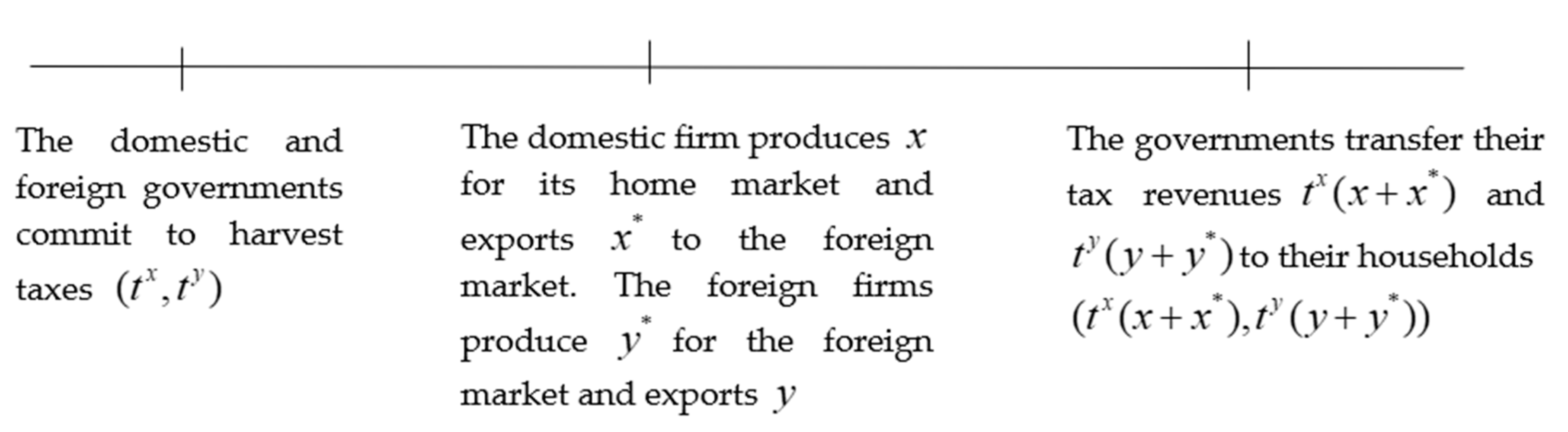
We formulate a policy setting game. The timing of the game is that (1) the governments in the two countries simultaneously choose harvest taxes; (2) the firms simultaneously choose domestic and export production. Their output choices determine the market quantity and price, wood harvest, profits, and consumer surplus; and (3) the governments transfer the tax revenues to domestic households.
Figure 1 depicts the timeline.
We look for a subgame perfect Nash equilibrium (SPNE) in the game. In order to identify the set of SPNEs, we use backward induction from the output stage to the policy stage (the transfers household receive in the third stage does not affect their demand since we assume that demand is only a function of price and not income. This is a reasonable approximation when consumer spending on the final good is a small share of total consumer spending). We let
and
y denote the domestic and foreign sales in the home market, and
and
denote the domestic and foreign sales in the foreign market (see
Appendix B for all notations). In equilibrium in the case of trade the total quantity demanded in the domestic country is thus
and the foreign quantity demanded is
Where necessary, we use superscripts
and
to distinguish the domestic and foreign tax, and use the superscripts “
A” and “
RD” to denote the autarky and reciprocal dumping outcomes (notice that if we impose symmetry on the countries we have
). Finally, in order to derive analytical results, we assume that the inverse final goods demand is
with
and that the environmental utility loss is
where
. We also assume that the parameters are such that the equilibrium harvest tax is positive.
3.1. The Output Stage
In the output stage under autarky, the profit and household utility net of the profit are:
Under reciprocal dumping, the profits of the domestic and foreign firms, along with household utility net of the profit, are:
Lemma 1. - (i)
Under autarky, the market quantity and wood harvest, price, profit, consumer surplus, and the marginal profit, consumer surplus, and environmental loss effects of the harvest tax are: - (ii)
Under reciprocal dumping, the market quantity, price, profit, consumer surplus, domestic wood harvest, and the marginal profit, consumer surplus, and environmental loss effects of the harvest tax are: - (iii)
Consider any given constant and symmetric harvest tax t that the countries may set. Then the harvests and the marginal profit, consumer surplus, and environmental benefits due to the tax before and after trade, can be ranked as follows:
The intuition behind the rankings in part (iii) is as follows: opening up to trade increases the quantity of production because the firms engage in Cournot-competition instead of producing the monopoly quantity, i.e., market competition increases. The marginal profit loss due to the tax increases after trade because the firm—which is taxed per production unit—produces a larger quantity and loses market share both at home and abroad when its marginal cost increases. On the other hand, the consumer surplus loss due to the tax decreases because, after trade, the consumers can purchase the final good from abroad and the price increase due to the tax is smaller. Finally, the harvest tax reduces the marginal utility loss from forest use more effectively after trade because the firm produces more output and the forest stock is smaller. The smaller forest stock implies that the marginal value of the forest and the marginal environmental benefit of the harvest tax are larger after trade.
3.2. The Policy Stage
In the policy stage, the government chooses the harvest tax to maximize the weighted sum of profits, wages, consumer surplus, the utility loss from forest use, and tax revenues:
with the optimality condition:
Lemma 2 defines the optimal harvest taxes under autarky and reciprocal dumping.
Lemma 2. The equilibrium harvest taxes under autarky and reciprocal dumping solve: In the next two propositions, we study the effects of different parameter changes on the regulation level as measured by the harvest tax after conditioning on the trade situation.
Proposition 1. Conditional on autarky, increases in the strength of the firm lobby effort and the wage level decrease the harvest tax. An increase in the demand for the final goods increases the harvest tax. That is: Proposition 2. Conditional on reciprocal dumping, increases in the strength of the firm lobby, the wage level, and the transportation cost decrease the harvest tax. An increase in the demand for the final goods increases the harvest tax. That is: The intuition for Propositions 1 and 2 is relatively straightforward. Under autarky, as well as trade, if the government is more industry-biased, it sets a smaller harvest tax in order to increase firms’ profits. A higher wage level decreases the production level and, therefore, the magnitude of the environmental externality (the forest loss). The marginal cost of the tax in terms of foregone profit and consumer surplus stays constant, while the marginal benefit associated with reducing the forest loss is smaller. The government, therefore, decreases the tax. Conversely, if demand for the product is strong, the production level and the environmental externality are large, causing the government to increase the tax to counteract the externality. A higher transportation cost decreases the production level and, therefore, the magnitude of the environmental externality. Since the marginal benefit associated with reducing the forest loss is smaller, the government decreases the tax. The next proposition studies how opening up to international trade affects the harvest tax.
Proposition 3. Trade increases the harvest tax () regardless of the industry bias.
Proposition 3 shows that international trade increases the harvest tax. The introduction of international competition between the firms and governments causes a regulatory race to the top. As the industry bias increases, the government decreases the harvest taxes under autarky, as well as in the trade regime (see Propositions 1 and 2). However, the tax under trade always exceeds the autarky tax. In the simulation we present below, we further find that the magnitude of the upward tax jump due to trade increases with the industry bias. In the next proposition, we show that, as long as the government is not biased against the industry, the upward tax jump is also large enough to decrease production.
Proposition 4. If the government maximizes national welfare and the shipping cost is zeroit implements the same production level under trade as in autarky. If the government is biased against the industry and the shipping cost is small, it implements more production under trade. If either the shipping cost is positive or the government is industry biased, it decreases production under trade.
The fact that the production-level under trade is typically smaller than under autarky unless the government is biased against the industry, implies that the tax increase must be substantial in the sense that it is bounded away from zero. The reason we know this is that Lemma 1 shows that for any given harvest tax, going from autarky to trade causes a discrete increase in production. In order for the equilibrium production level to fall, therefore, the tax must increase significantly.
In order to see why welfare-maximizing governments keep the production level equal to the autarkic level as long as the shipping cost is zero, assume that the wage is . Thus, the only welfare cost from producing is the environmental cost of the resource harvest . Under autarky, a welfare-maximizing government increases the harvest tax until the marginal loss of market surplus —equivalently, the marginal drop in the sum of profits and consumer surplus or the marginal “stripe” under the demand curve—equals the marginal environmental benefit. International trade does not change the marginal benefit. However, it also does not change the marginal decline in the sum of profit and consumer surplus: when the government in the trading economy implements a unit production decline, the firm sells 0.5 units less in each market. The fall in domestic welfare is, therefore, half of the marginal willingness to pay, , plus the change in the profit portion of the market surplus that is appropriated by the foreign firm. Since the foreign firm sells half of the output in the domestic market, the change in the foreign profit is , where is the price increase when the domestic firm cuts sales by 0.5 and the foreign firm respond with a sales change . The domestic welfare decline linked to home market sales is, therefore . The price also increases by in the foreign market, which increases the domestic export profit on existing sales by . Finally, the 0.5 decline in the export quantity costs the home country in export revenues. The total domestic welfare change linked to export sales is, therefore, . The overall domestic welfare change is, therefore , which is the same as under autarky. Since the welfare-maximizing government continues to earn and lose from quantity reductions, it implements the same production and market quantities under trade and autarky. The reason that it nonetheless has to increase the harvest tax (as Proposition 3 demonstrates) is that the firm’s demand curve is more elastic under trade. If the government kept the harvest tax rate constant, the firm would increase production. Formally, Lemma 1 shows that opening to trade increases production at every initial harvest tax, so stabilizing production requires a tax increase.
Once we allow the shipping cost to be positive, the marginal benefit to society from exporting decreases. Since the marginal environmental cost of increasing production is the same, but the marginal benefit decreases due to the deadweight loss from shipping, the government prefers to decrease production below the autarkic level.
Finally, what happens when the government is industry-biased? In this case, the government values the after-tax profit at and perceives a loss per tax unit collected in addition to the quantity effects of the tax. As Propositions 1–2 show, it, therefore, decreases both the autarkic tax and the tax under trade, which increases the respective quantities. The reason that the equilibrium quantity under trade increases less rapidly with the industry bias than the equilibrium quantity under autarky reflects the fact that, under trade, the firm’s demand curve is more elastic. As a result, the tax cut needed to encourage the firm to produce an additional unit is smaller. Formally, the proof of Lemma 1 shows that production under trade is , so increasing production by a unit requires . In autarky, so increasing production by a unit requires a larger tax cut. From another perspective, the marginal profit gain from output expansion is smaller under trade, which erodes the government’s incentive to subsidize the firm.
3.3. The Welfare Effects of Trade
We can express the welfare change due to trade as a function of the output levels. In order to do so, we will follow Burguet and Sempere [
13] and write welfare as:
which is the area under the demand curve minus the social cost of producing and exporting. The social cost of producing and exporting equals the wage cost
plus the environmental utility loss
plus the shipping cost when the country exports
output units. Once we substitute for the linear demand function and the environmental loss function, substitute the quantities from Lemma 1, and substitute the taxes from Lemma 2, we can express the welfare change as follows:
Proposition 5. The welfare change due to trade is:where:
implicitly define the optimal output quantities and harvest taxes. If the government maximizes national welfare and the shipping cost is zero
, the welfare change is zero. The absolute welfare levels are
and
, where the terms on the right-hand side are defined above.
The welfare effect of trade is theoretically ambiguous. On one hand, just as in the original Brander and Krugman [
3] model of trade with reciprocal dumping, the firms ship identical goods to each other’s markets. While the exports increase competition, it is socially costly to ship identical goods in both directions. In the present model, when , as Proposition 4 shows, the governments keep the trade quantities equal to the autarkic quantities, so the welfare change is just the two-way shipping cost,
with strict inequality unless
Thus, the reciprocal-dumping-driven trade decreases welfare. As the governments become industry-biased, however, so
increases above unity, the autarky quantity
increases above the national-welfare maximizing level, which decreases the autarkic welfare level. The fact that the welfare level under autarky is relatively low opens the possibility that trade can increase welfare. In the numerical example, we present below we show that, although international trade liberalization with a zero-shipping cost has zero welfare effect, trade liberalization with industry-biased governments can potentially increase welfare.
Before we proceed to the simulation, we believe that it may be interesting to compare Propositions 4–5 to the closely related results in Kennedy [
12] and Tanguay [
27], who both study a similar two-country model where the governments are welfare-maximizing and the transport cost is zero. If we similarly assume that the governments maximize welfare and that the transport cost is zero (
), Propositions 4–5 imply that (a) the governments implement the same production levels under autarky and trade. Moreover, (b) since the governments maximize national welfare and there are no environmental spillovers [
12,
27], the production quantities maximize both national and global welfare. The model in Tanguay [
27] yields the same prediction: comparing the solution for the Nash equilibrium environmental taxes and production quantities in Tanguay’s Equations (21) and (25) with the first-best solutions in Equations (34) and (37) shows that the solutions for both variables coincide whenever (like here) there is no transboundary production spillover. In contrast, Kennedy [
12] finds that the two-country equilibrium without transboundary externalities leads to downward-distorted pollution taxes and, therefore, excessive production. The reason is that Kennedy’s model assumes that the firms in the two countries can invest in pollution abatement, which would correspond to investing in a resource-conserving-production technology in the present paper. When we solved Kennedy’s model without the possibility of investing in abatement, we found that, just as in the model here and Tanguay [
27], the trade outcome is efficient.
3.4. An Example and Some Additional Results
In order to illustrate the results in Propositions 1–5 and to demonstrate some additional properties the solution may have, we conduct simulations.
Figure 1 depicts the simulation results when we assume that
. Thus, we assume that the inverse demand for the final good in each country is
, the shipping cost is zero, the wage is one, and the environmental loss is
. The reason why we set the shipping cost to zero is that it allows demonstrating the results in Propositions 4–5 that, if the governments maximize national welfare and face a zero shipping cost (
and
) they implement the same production quantities under trade and autarky, so opening to trade has zero welfare effect.
Figure 2a depicts the government’s marginal benefit from the harvest tax in Equation (7) under autarky, as well as trade when the governments maximize national welfare
. The marginal benefit of the tax is always higher in the reciprocal dumping or trade scenario compared to the autarky scenario. The equilibrium taxes are about
under autarky and
under reciprocal dumping. In
Figure 2b we depict the optimal taxes as the industry bias gradually increases from
to
. As we showed analytically in Propositions 1–3, the taxes decrease with the industry bias, but the tax remains higher under trade than in the autarky scenario. In
Figure 2c we depict the corresponding production quantities as the industry bias increases from 1 to 4. Note that, although we do not explicitly depict the environmental utility loss
, our assumptions that
imply that the utility loss increases at an increasing rate along with the production quantity. Consistent with Proposition 3, the output quantity is smaller under trade unless
. It is also interesting to note that the upward tax jump and downward quantity jump due to trade in panels b and c increase with the industry bias. The reason is that, as the industry bias increases, the tax decreases more rapidly, and the production quantity increases more rapidly, in the autarky scenario than in the trade scenario. Unfortunately, we have been unable to establish the analytical counterparts to these results, that is, to demonstrate that
is always positive and
is always negative.
Finally,
Figure 2d depicts the welfare change due to trade as the industry bias increases. As Propositions 4–5 jointly demonstrate, when
and
, trade has zero welfare effects since the production levels remain unchanged and the new two-way shipping of goods due to trade is costless. As the industry bias increases, however, the governments gradually decrease the harvest taxes under both autarky and trade. Since the autarky quantity is above the national welfare-maximizing level, trade opening is able to increase welfare. Despite the fact that industry bias can increase the change in the absolute welfare level due to trade, however, it still decreases the absolute welfare level. In other words, industry bias still decreases absolute welfare.


