Article

Management of Plant Growth Regulators in Cotton Using Active Crop Canopy Sensors

by
Rodrigo Gonçalves Trevisan
*,
Natanael Santana Vilanova Júnior
,
Mateus Tonini Eitelwein
and
José Paulo Molin
Precision Agriculture Laboratory, Department of Biosystems Engineering, Luiz de Queiroz College of Agriculture, University of São Paulo, Piracicaba 13418-900, São Paulo, Brazil
*
Author to whom correspondence should be addressed.
Agriculture 2018, 8(7), 101; https://doi.org/10.3390/agriculture8070101
Submission received: 1 June 2018 / Revised: 24 June 2018 / Accepted: 25 June 2018 / Published: 2 July 2018
(This article belongs to the Special Issue Precision Agriculture)

Abstract

:
Factors affecting cotton development present spatial and temporal variability. Plant growth regulators (PGR) are used to control vegetative growth, promote higher yields, better fiber quality, and facilitate mechanical harvest. The optimal rate of PGR application depends on crop height, biomass, and growth rate. Thus, the objective of this study was to evaluate optical and ultrasonic crop canopy sensors to detect the crop spatial variability in cotton fields, and to develop strategies for using this information to perform variable rate application (VRA) of PGR in cotton. Field trials were conducted in Midwest Brazil during the 2013/2014 and 2014/2015 crop seasons. Two optical and two ultrasonic active crop canopy sensors were evaluated as tools to detect crop variability. On-farm trials were used to develop and validate algorithms for VRA based on within-field variations in crop response to PGR applications. The overall performance of the sensors to predict crop height and the accumulation of biomass in cotton was satisfactory. Short distance variability was predominant in some fields, reducing the performance of the sensors while making current technology for variable rate application of PGR inadequate. In areas with large scale variability, the VRA led to 17% savings in PGR products and no significant effect on yield was observed. Ultrasonic sensors present can be a low-cost alternative to implement variable rate application of PGR in real time.

Graphical Abstract

1. Introduction

Cotton (Gossypium ssp.) is among the most important fiber crops, with approximately 35 million hectares grown throughout the world. Global demand has gradually increased since the 1950s, with an average annual growth of 2%. About 350 million people around the world carry economic activities related to cotton, making it one of the 20 most important commodities in the world market in terms of its value [1].
Brazil produces about 1.7 million tons of cotton lint per year, being placed among the top five global producers, after China, India, Pakistan, and the United States. Brazil is also the fourth largest exporter in the world, with an area planted with cotton in the last five crop seasons averaging 1 million hectares, with some variations due to the market scenarios for the sector and production costs [2]. The national average cottonseed yield surpassed the 4000 kg ha−1 mark in the 2014/2015 season, which makes Brazil the country with the highest yields of dryland cotton cultivated in the world. Although this average is reasonable, many producers have focused on improving techniques to increase crop productivity by adopting higher levels of technology.
The cotton height must be periodically managed to decrease the abortion of reproductive structures by carbohydrates competing with the vegetative growth [3]. Cotton growth and its response to application of plant growth regulators (PGR) highly depends on temperature and water availability. The decisions about PGR rate, timing, and the general crop management remains a challenge for growers, especially due to spatial variability of soil conditions, which demands the use of variable rate application (VRA) of nitrogen and PGR.
Crop canopy vegetation indexes have been used to detect infield variability. Active and passive optical reflectance sensors mounted in various platforms have shown good performance to predict biomass, plant height, height-to-node ratio, nitrogen nutrition status, crop maturity, and lint yield [4,5,6,7,8]. The performance of sensors can vary throughout the crop season, due to crop canopy changes and management practices. Good results are usually found in early season (pin-head square to early bloom), but poor performance may occur due to the known effect of signal saturation when used later in the season, due to dense canopy and changes in the spectral signature of the plants.
Normalized difference vegetation index (NDVI) and plant height have a good correlation with stem mass and leaf mass during the early and late crop stages, but not during mid-season of cotton cycle [9]. In mid-season, more than 90% of NDVI values exceeded 0.8, and nearly half were above 0.9, which showed saturation of optical sensor. PGR applications promote increased chlorophyll concentration and reduced leaf area, which can also affect the sensor readings [10]. Unlike optical readings, crop heights have shown a good correlation with crop biomass through the entire season, even after peak bloom, which could be used to improve the detection of infield variability. This could allow farmers to make better decisions and assist in variable rate application of PGR.
Plant height is an important deciding factor for application of PGR. Nevertheless, other crop parameters can also be used to guide PGR application decisions, and may even be better than crop height growth in some circumstances. The height-to-node ratio (HNR) is calculated by dividing plant height by the total number of main stem nodes, and is equal to the average internode length. The height of the top five nodes is an estimate of current crop growth rate, and can be a good indicator of rank growth and the need to apply higher rates of PGR. Plant growth rate was shown to be inversely correlated to its leaf PGR concentration. Therefore, the total dry biomass should also be accounted when deciding PGR application rates [3].
Cotton production systems can be improved with better understanding of the interactions between soil and crop spatial variability and its influences on the best management strategy regarding PGR application rates. Thus, the objective of this study was to evaluate optical and ultrasonic crop canopy sensors to detect crop spatial variability in cotton fields, and to develop strategies for using this information to perform variable rate application of plant growth regulators in cotton.

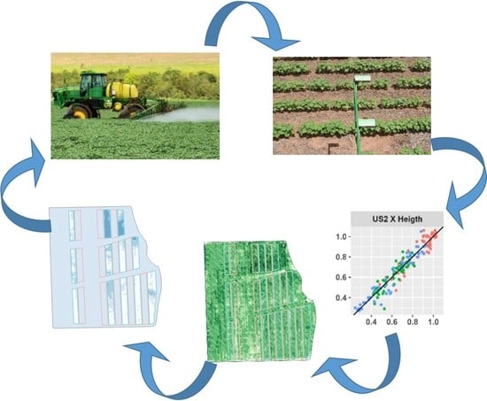
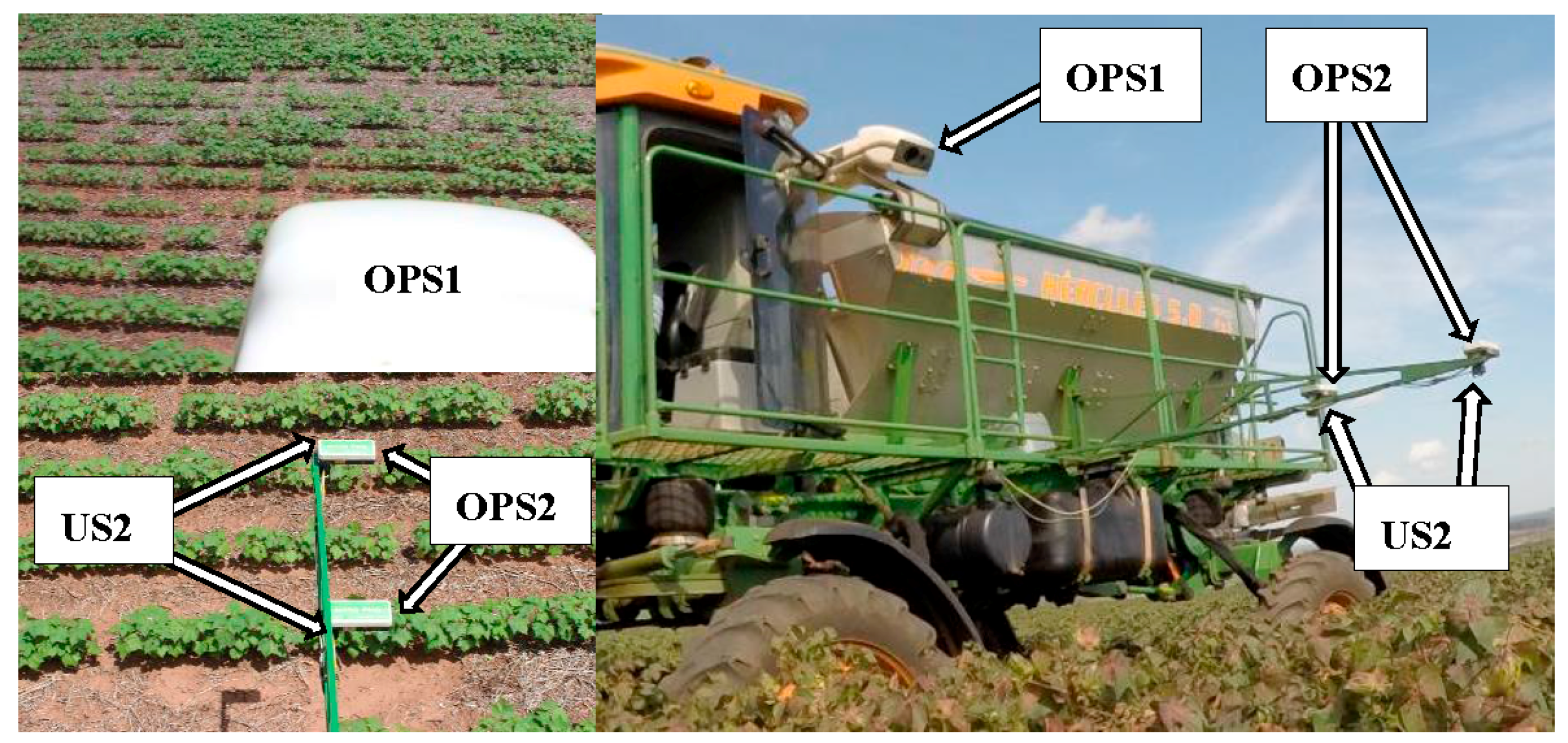
2. Materials and Methods

Fields trials were located in the states of Goiás (2014 crop season—GO) and Mato Grosso (2015 crop season—MT), Midwest Brazil. Five fields were studied for all research protocols. The soil in the experimental fields ranged from clay Oxisols to sandy loam Quartzipsamments, with different levels of spatial variability in soil clay content. More details of the experimental fields are presented on Table 1.

2.1. Sensor Performance to Predict Crop Parameters

Two types of optical sensor systems were used (Table 2). The first optical sensor system—OPS1 (N-SensorTM ALS, Yara International ASA, Dülmen, Germany), was installed above the vehicle cabin and the readings were taken from an oblique position. The OPS1 data acquisition was made in Yara N-Sensor software running on Microsoft Windows operating system. The sensors measure canopy reflectance in red edge (730 nm) and near infrared (760 nm), and a scaled logarithmic difference of reflectance at the two wavelengths was used as the vegetation index in all comparisons [11].
The second optical sensor system, OPS2 (Crop Circle ACS-430, Holland Scientific, Lincoln, NE, USA), was mounted to take readings directly above the crop canopy. The OPS2 was integrated with the GEOSCOUT GLS-420 mapping system (Holland Scientific, Lincoln, NE, USA) for data acquisition. The sensors measure canopy reflectance at three wavelengths, but only the red edge (730 nm) and near-infrared (780 nm) were used to calculate the Normalized Difference Red Edge Index (NDRE), which was used in all comparisons.
In order to evaluate the optical sensors’ saturation problem, described above, and to test simpler and less cost-intensive technologies, ultrasonic sensors systems were developed and tested using the same conditions. The objective of these systems was to calculate plant height using the time of flight principle to measure the distance between the top of the canopy and the sensor (Table 3). The first system was US1 (Polaroid 6500, Minnetonka, MN, USA), with a working frequency of 49.4 kHz, using custom software for data acquisition by a data logger (CR 1000 Campbell Scientific, Logan, UT, USA). This system was used for 2013/2014 crop season, and one sensor presented malfunction problems in the last acquisition. Due to the difficulties of finding replacement parts, a new system was developed for the next season. The second system, US2 (HC-SR04, generic sensor), with a working frequency of 40 kHz, uses low-cost hardware commonly used in automation projects and data acquisition based on an Arduino® Mega 2560 (Arduino, Ivrea, Italy).
All sensors were installed in a high-clearance vehicle operating with a swath width of 30 m, at a maximum travel speed of 23 km h−1. The measurements were georeferenced using Global Navigation Satellite System (GNSS) receivers. In 2013/2014 crop season, an L1/L2 receiver without differential correction was used. The OPS2 and US1 were mounted on brackets 1 m externally of tire tracks in each side of the machine, and the OPS1 was mounted above the main cabin, with one sensor head facing each side of the machine (Figure 1). For the 2014/2015 crop season, real-time kinematic (RTK) receivers were used for data collection and referencing sample points. The US2 replaced the US1 used in the previous year. The sensor mounting positions were kept the same and one more sensing units of each OPS2 and US2 were added at each side of the machine, mounted on brackets 1.7 m externally of tire tracks.
All sensor data acquisition was made simultaneously in a single machine pass in each field. After data acquisition, sensor readings were averaged in polygons with 5 × 15 m to produce the variability maps. These dimensions were chosen based on the average distance between sensor readings and half the swath width. Based on the maps, 30 validation locations were selected in each field map in order to represent the entire range of crop variability. In each validation sample point, plant height was hand measured, and destructive plant samples of the aboveground biomass were taken by manually cutting and weighing a 1.0 m subplot consisting of three rows. Although the sampled area was different on narrow row and conventional row cotton, the number of rows was kept constant because the number of plants per sample was similar, due to the differences in plant population. During the 2013/2014 crop season, data acquisition and field sampling were repeated at five important phenological stages of cotton, representing the stages 51, 61, 71, 81, and 95 in BBCH scale [12]. One of the objectives of 2014/2015 crop season was to better understand how crop parameters useful for PGR recommendations interact with each other and with the sensor readings in different scenarios. For this reason, in addition to crop height and biomass, dry biomass, height of top five nodes, and the height-to-node ratio were evaluated at BBCH 71 phenological stage. The number of sampling points was also increased to 54 in each field.
Data obtained in the sampling points was submitted to descriptive statistical analysis and linear regression analysis, comparing each sensor performance for individual fields and sampling dates. Values of fresh biomass for the 2013/2014 crop season were transformed to squared roots before regression in order to meet the assumptions of data normality and homoscedasticity of variances. Results for this variable are presented after back transformation to original scale. All statistical procedures were performed using the R software, version 3.4.0 [13].

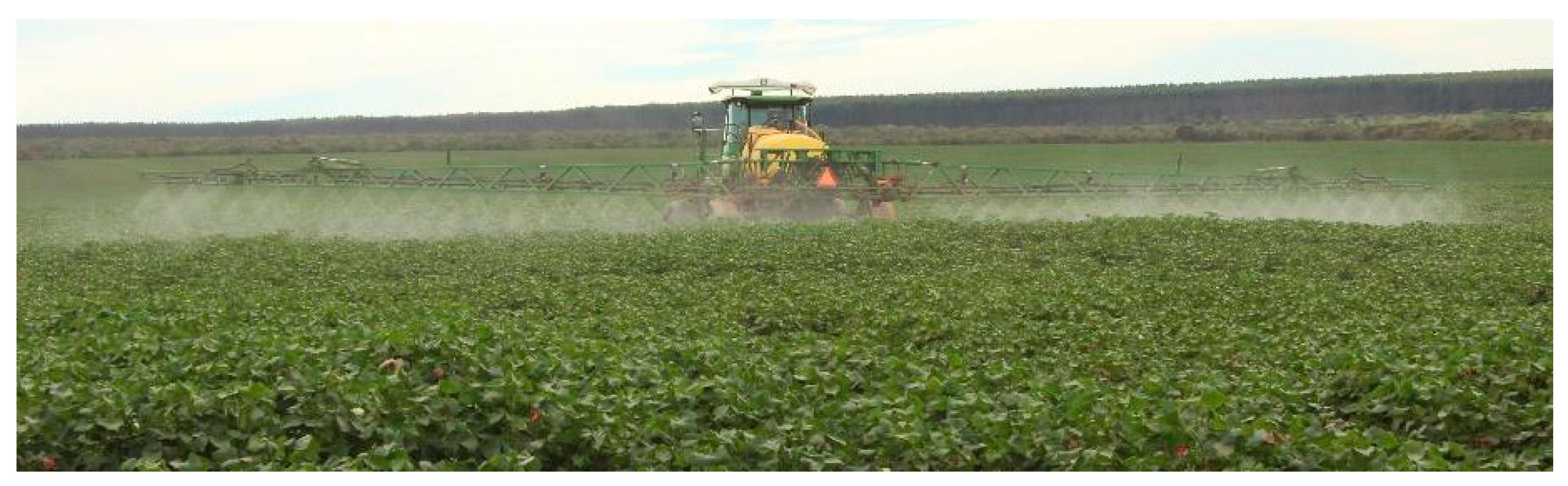
2.2. Variable Rate Application of PGR

The variable rate prescription maps of PGR and fruit ripener were created based on the crop variability detected by crop sensors, relations of crop parameters and sensor readings from this and previous works, and field evaluation of representative points before each application by crop advisors. The methodology used is similar to what was presented in [14], but instead of dividing the field into a few application zones, regression analysis was used to predict optimal PGR rate for every pixel, allowing rates to vary between 80 and 120% of the field average rate for each application. When the optimal rate was less than 50% of field average, the rate was set to zero. Rates between 50 and 80% were set to 80%, and rates greater than 120% were set to 120%, due to the sprayer variable rate limitations.
The experimental layout consisted of on-farm trials with 72 m wide swaths, and variable length according to field position. A random block design was used, with five blocks on narrow row field NF2, and 12 blocks on conventional row spacing field CF3. Each block had three sprayer passes made in variable rate, and another three with fixed rate. The block locations were chosen to represent the field variability, while keeping both treatments in similar conditions. Some parts of the fields were used for nitrogen, and variety trials and were not included in analysis. Prescription maps were transferred into the JD GreenStar 3 controller on a JD 4630 self-propelled sprayer (Figure 2). PGR application was done using nozzles Teejet DG 8003 VS Drift Guard Flat Spray Tip (Spraying Systems Co., Wheaton, IL, USA), spaced at 51 cm, using an average tank mixture rate of 60 L ha−1 at 20 km ha−1.
Cotton was harvested using JD 7760 cotton picker (John Deere, Moline, IL, USA), with Harvest Doc™ yield monitoring system. For the narrow row cotton, a variable row spacing (VRS) kit was used. Yield data was georeferenced using RTK positioning with an acquisition rate of 1 Hz and average speed of 2 m s−1, producing about one yield point per 10 m2. Yield data was filtered to remove locally extreme values, according to the spatial filtering methodology presented by [15], and then averaged to each plot to further statistical analysis. Variable rate prescription maps were prepared using QGIS version 2.14 [16]. All statistical procedures were performed using the R software, version 3.4.0 [13].

3. Results and Discussion

The proposed methodology allowed the successful data acquisition and performance evaluation for most of the comparisons (Table S1). All results are presented for single crop stage evaluation, focusing on the information most useful for decision making at crop management level. Data logger connection presented some problems and generated missing data points for the OPS2 on CF1 in the BBCH 51. No data acquisition for US1 at BBCH 95 was caused by problems with the sensors. All problems presented on 2013/2014 crop season were fixed, and no data was lost on 2014/2015 crop season.

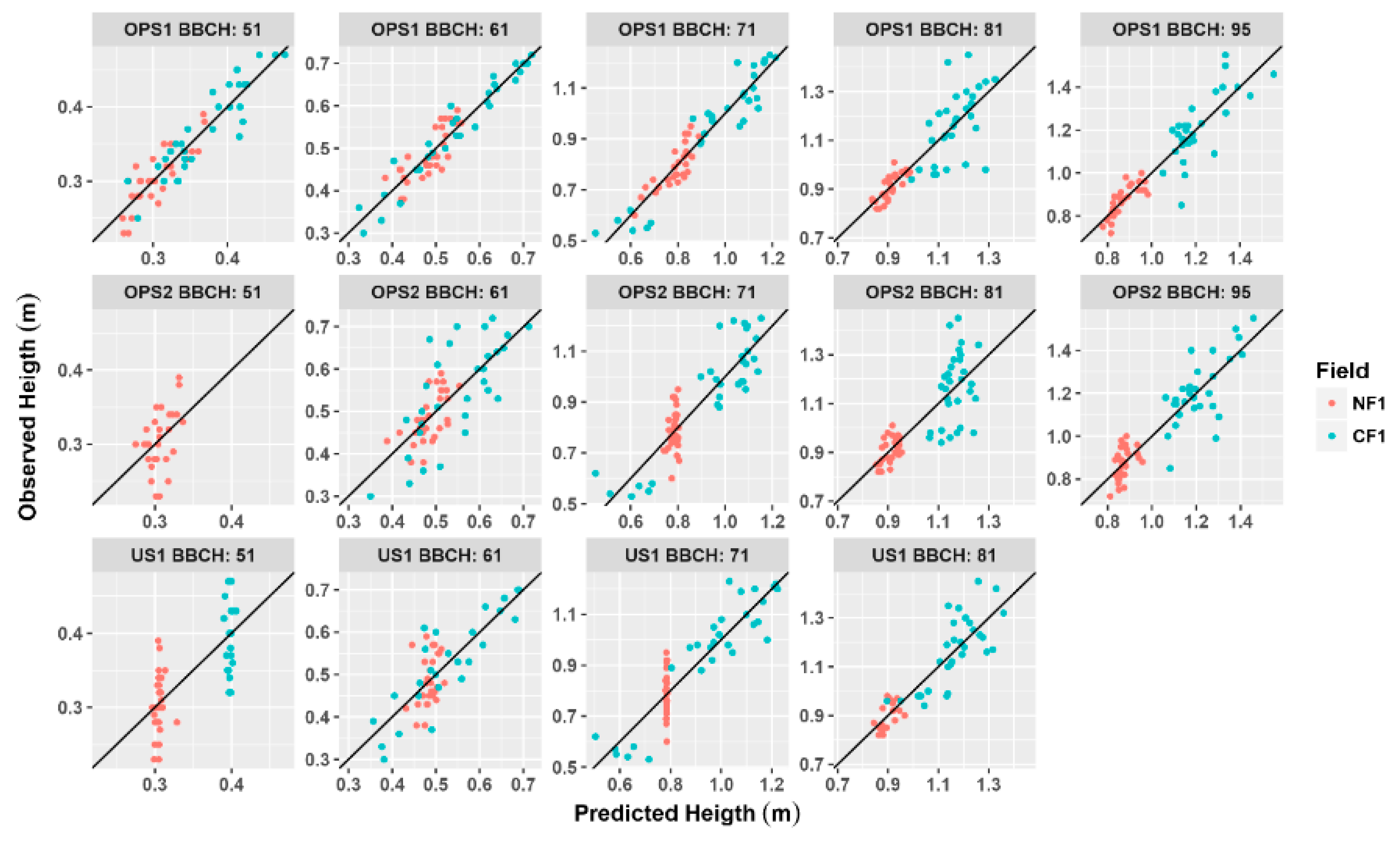
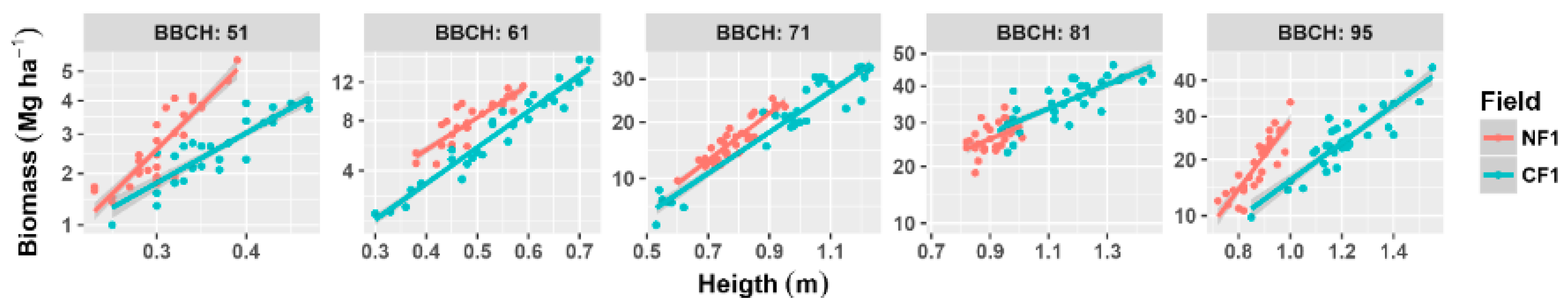
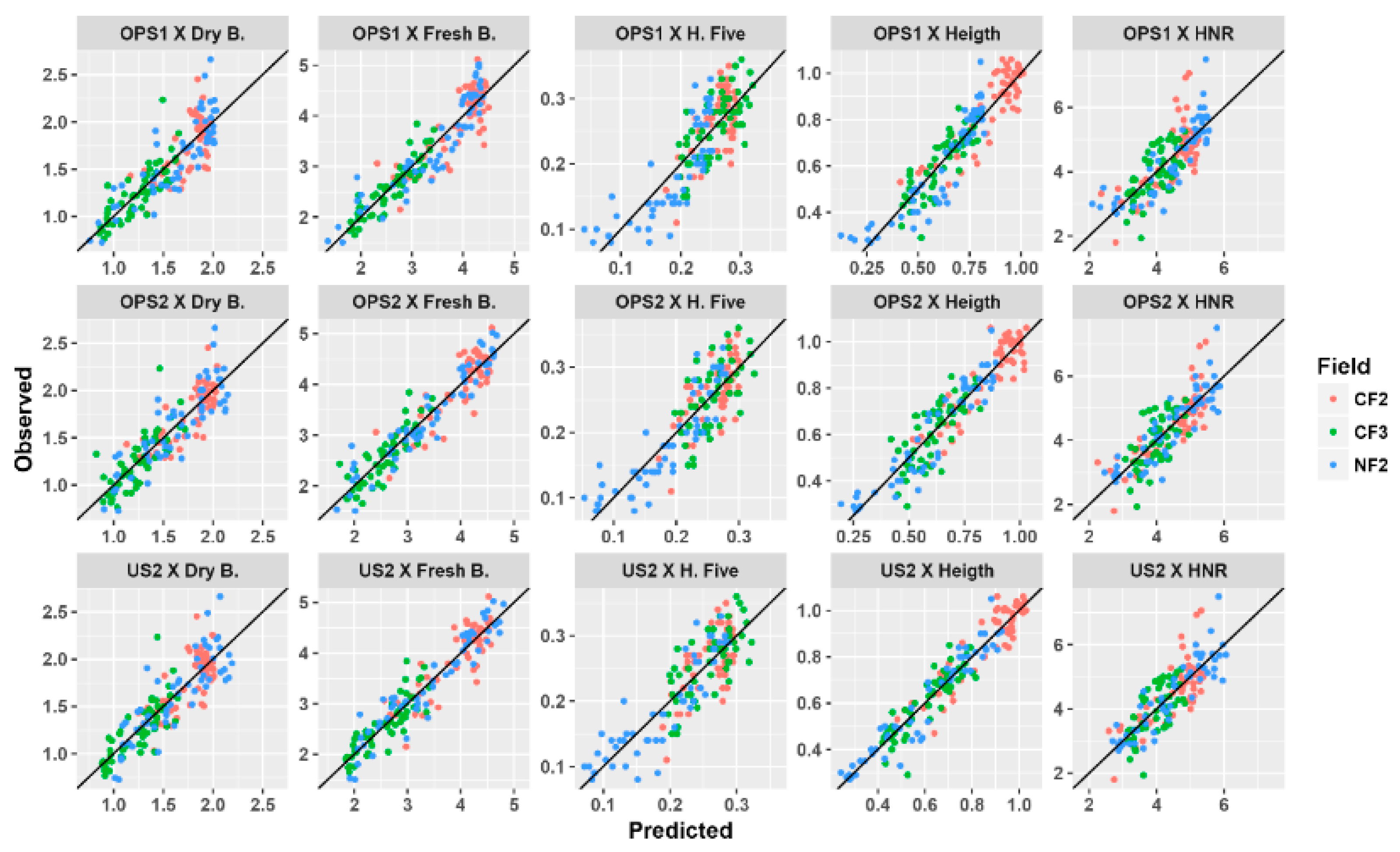
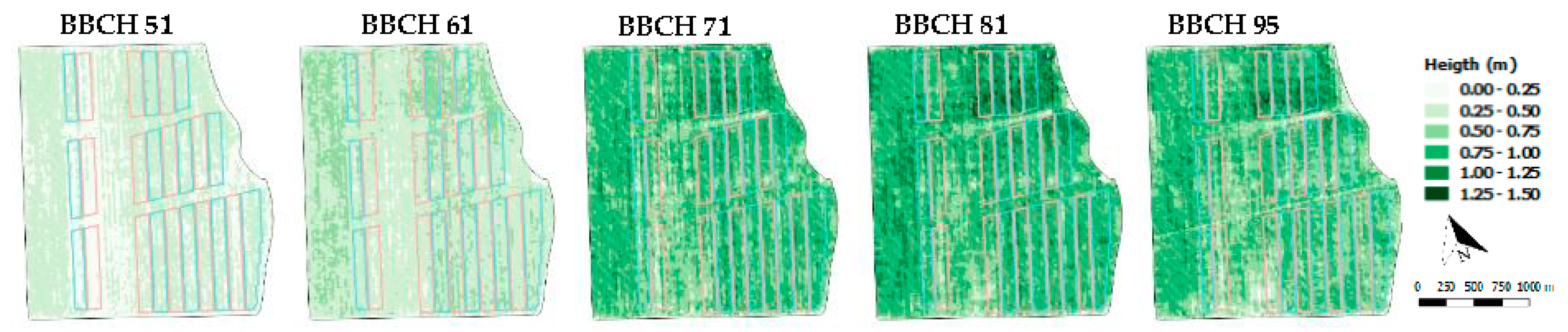
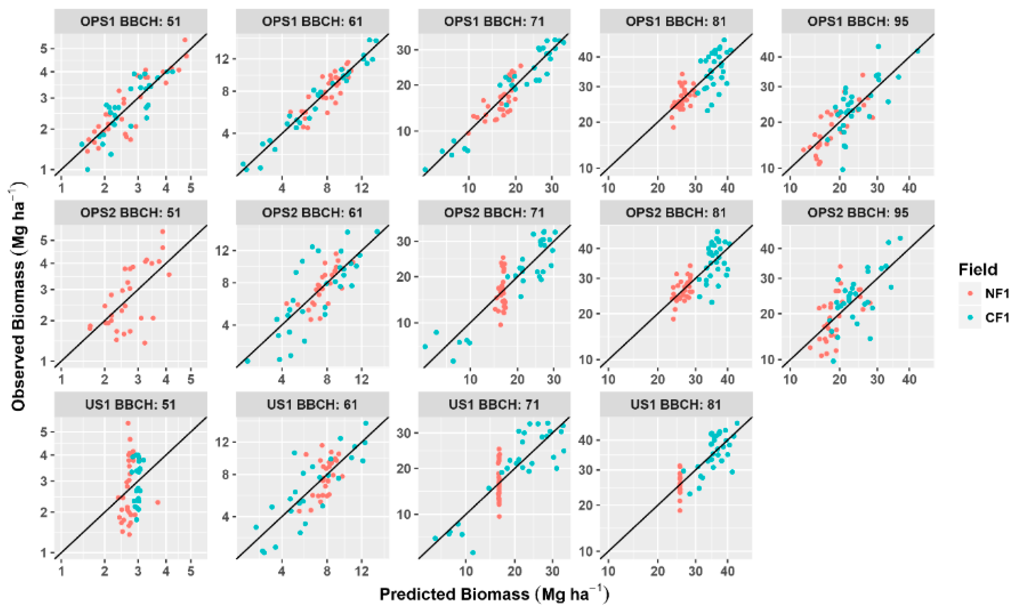
3.1. Sensor Performance to Predict Height and Biomass in Different Crop Stages

The two fields used for data acquisition in 2013/2014 presented different scenarios of spatial variability. The NF1 was overall homogeneous, with short scale variability caused by plant population variability, due to excess soil moisture during seeding (Figure 3). The CF1 presented more large-scale variability caused by differences in soil clay content and water retention potential. The range of variability on CF1 was about three times larger than on NF1. Therefore, the differences in sensor performance are related to the differences in spatial variability of these particular fields, rather than row spacing and crop system.
The relation of biomass and crop height was dependent of the crop system and phenological stage (Figure 4). A greater increase in biomass was observed for each unit of increased height in NF1 than in CF1, which is due to the large plant population used in narrow-row cotton, allowing a fast accumulation of biomass. This relation forms the basis of using optical sensors to predict crop height. The OPS1 showed the best overall performance (Table 4, Figure A1 and Figure A2 in Appendix A). This sensor had a higher advantage due to its large footprint, being less affected by row-to-row variability of the fields. This is the main reason for the large differences in performance observed between OPS1 and OPS2. The small footprint of OPS2 generated more noisy data, capturing the variations between plants, in contrast to the overall field variability. The same applies to US1, which presented regular performance on CF1 and insufficient performance on NF1, due to this field’s short-scale variability.
The effect of the crop variability magnitude can be better observed when relating the coefficient of determination (R2) with the root-mean-squared error (RMSE) in each crop stage. Even with large differences in R2, the RMSE values are consistently similar among sensors in each evaluation stage. The maximum RMSE observed for crop height were in OPS2, with 0.08 m in NF1 and 0.13 m in CF1, which means that the sensor can provide good auxiliary information when large variability is present.
The worst performance of optical sensors was observed at BBCH 81, which agrees with the results obtained by [9]. The high volumes of biomass accumulated at this stage induce a saturation effect on vegetation indexes; moreover, there are also plants in different phenological stages induced by stresses due to water limitation. The US1 presented better performance than the optical sensors at this stage on CF1, however, the best obtained R2 of 0.56 was lower than the values obtained in the evaluation at the previous BBCH, which were above 0.80 for all sensors.

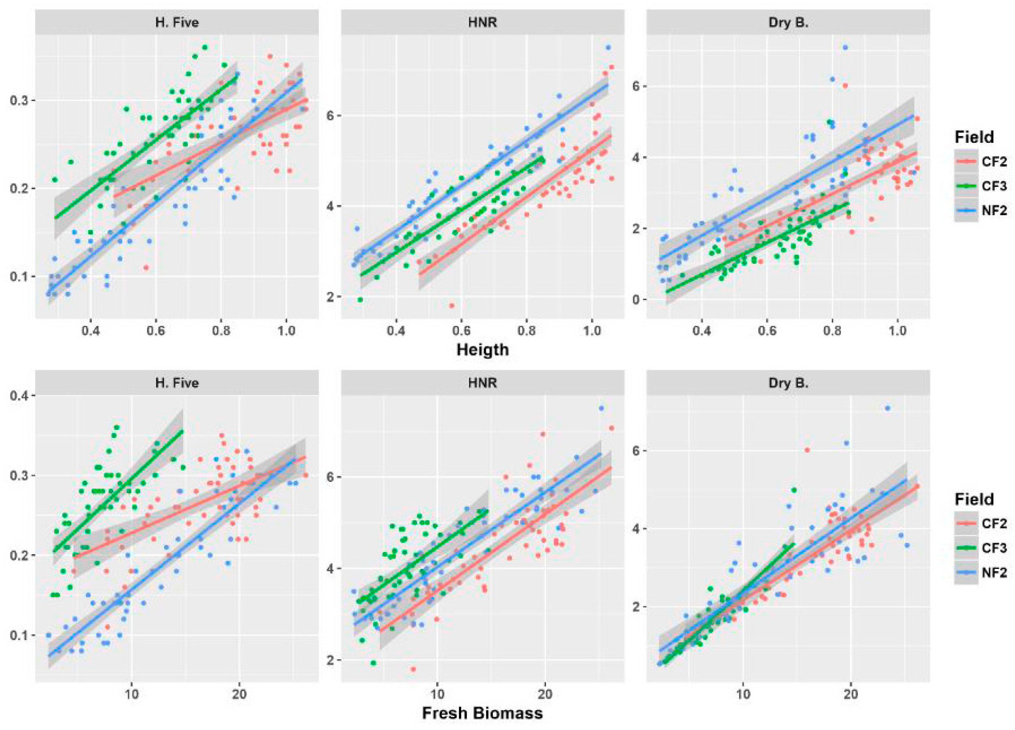
3.2. Sensor Performance to Predict General Crop Parameters

The relation among crop parameters depends on the crop system and the field (Figure A3 and Figure A4). Some parameters may present better stability to be used for general recommendations across different fields or even crop seasons. Nevertheless, when we consider a single field and crop stage, the parameters are correlated, and the characterization of field variability will be similar if based in any of these parameters.
Better control of data acquisition and sample locations was implemented using real-time kinematic (RTK) technology to avoid the effect of small-scale variability observed on 2013/2014 crop season. With this methodology, more stable results were obtained (Table 5 and Figure 5). Although this was important to better evaluate sensor performance while avoiding other effects, it does raise the question of whether the considered spatial resolution is enough to manage spatial variability effectively.
The consistency of RMSE values for different sensors and fields is to be highlighted again. The estimation of crop height using any of the sensors presented an RMSE inferior to 0.08 m in all fields. The US2 presented the best performance in estimating crop height, and very similar results to the optical sensors for the other parameters. The range of variations that can be observed in Figure 5 contributed to the good performance observed on these fields. The points representing field NF2 are well distributed over the entire range of values, and this was the field with the best results.

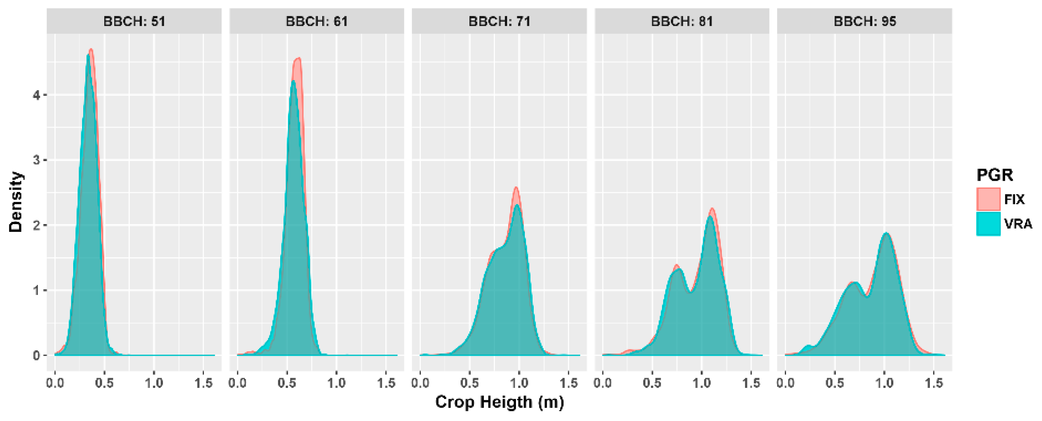
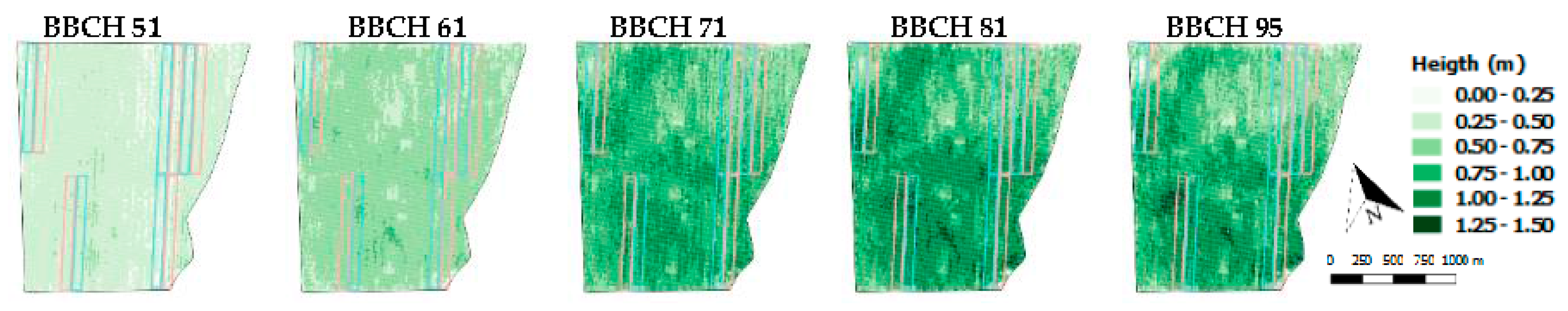
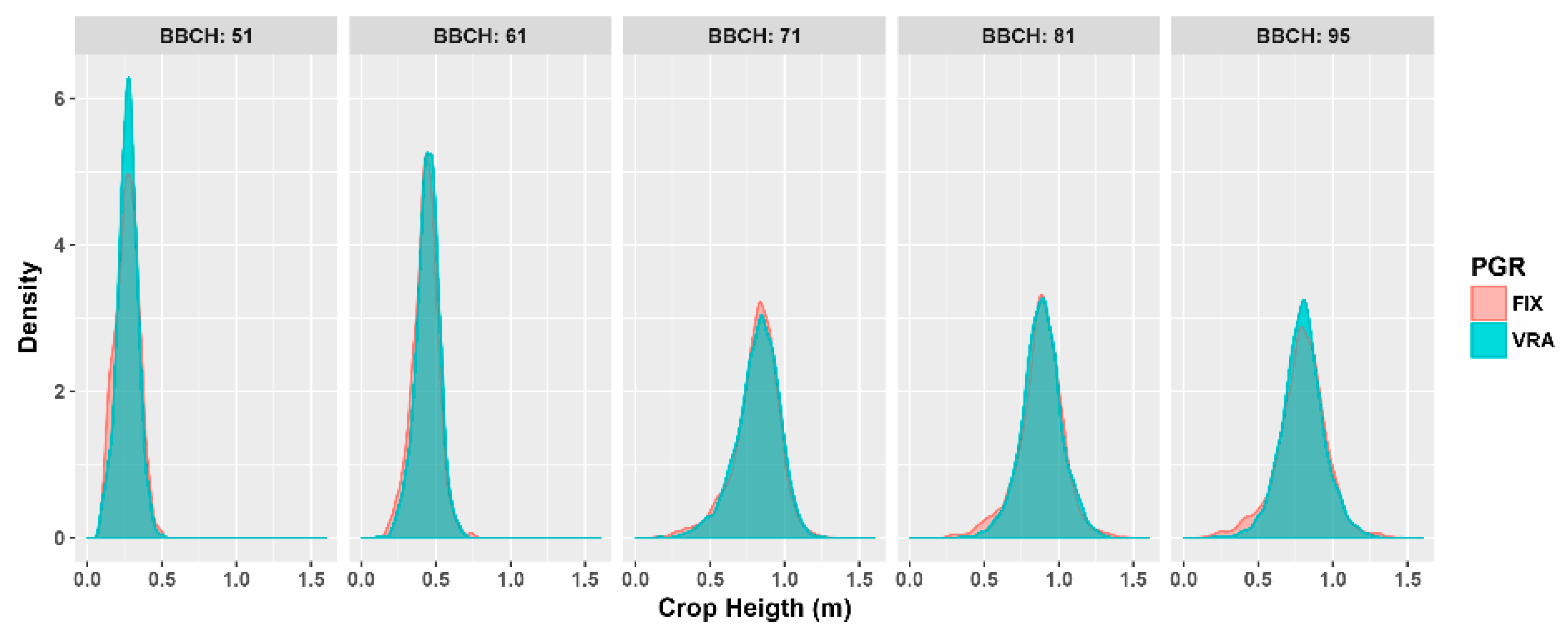
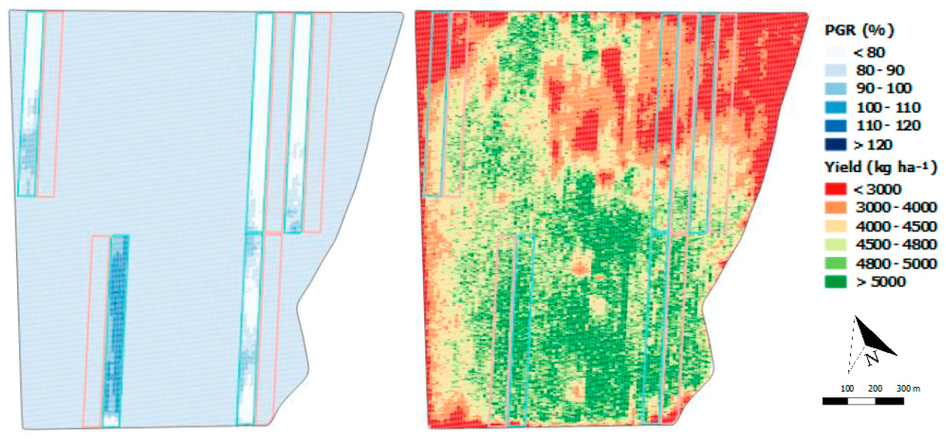
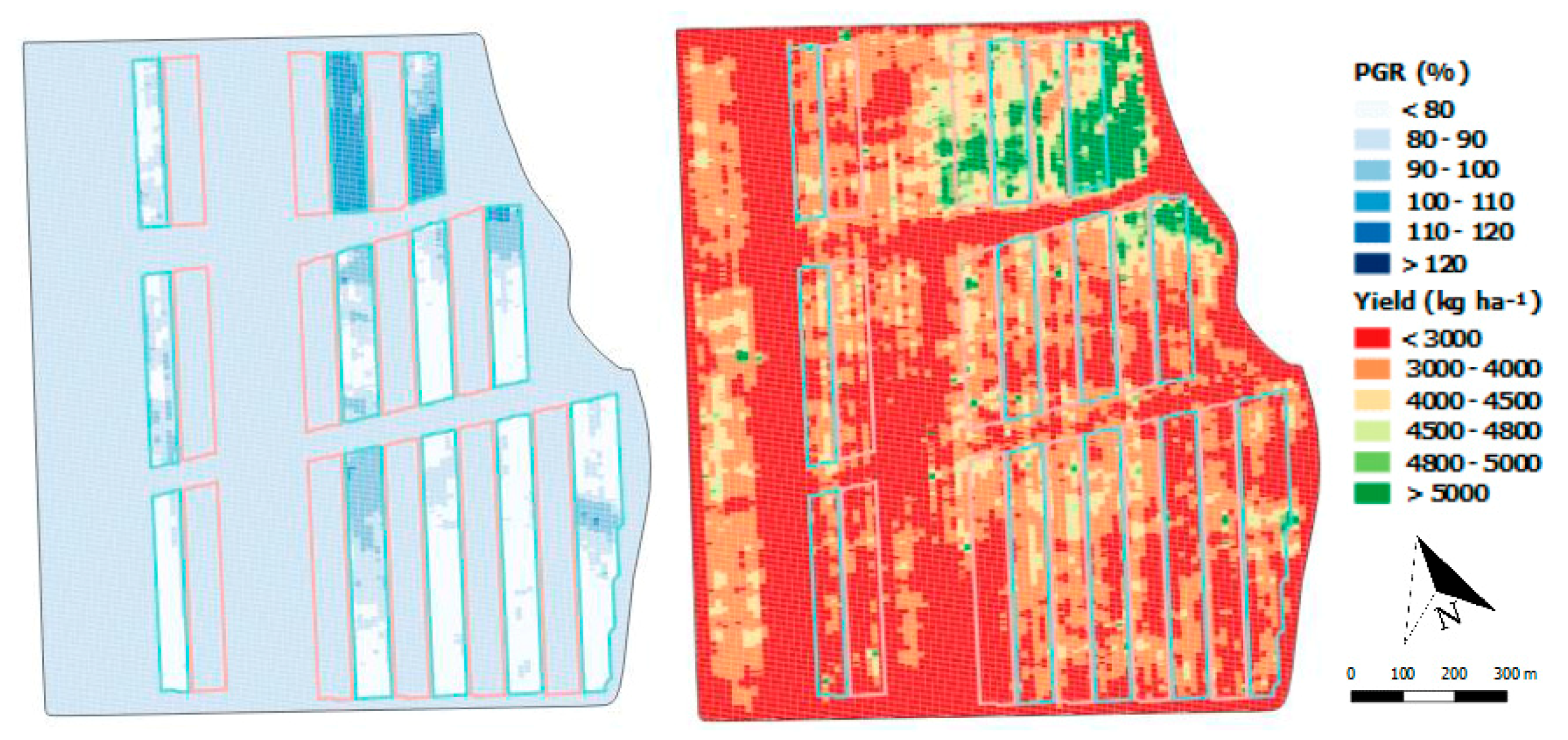
3.3. Crop Response to Variable Rate PGR

Crop height was not statistically affected by the use of fixed rates or VRA of PGR in the two experimental fields. The variations in PGR rates were not sufficient to reduce the variations in crop height when compared to fixed rate application (Figure 6). One of the reasons for this is the machine limitations, due to pressure variation constraints to control water flow [17]. This limitation could be overcome with other variable-rate spraying technology, such as pulse wide modulation at individual nozzles. A direct injection system could also allow for greater variations, but the difficulties with short scale variations would still need to be addressed in further studies.
Another important reason for the lack of response may be the timing of decisions. In these fields, the most important factor limiting crop development and yields was the soil water retention potential. The crops were rainfed, and enough rain, totaling more than 800 mm, was well distributed from January to April, until the crop reached BBCH 61. After that, the rain stopped, and the crop had only the water present in the soil to finish its cycle.
The bimodal distribution of plant height, which can be seen in Figure 6, was caused by the large differences in soil characteristics of NF2 (Figure A5). In the soils with low water retention potential, the crop stopped growing due to water limitation, even with the zero-rate of PGR applied. This contributed to PGR savings, but the crop uniformity was not improved. In the regions with high water retention potential, the opposite was observed. Even with 20% increase in PGR rates, the crop presented rank growth in some regions of the field (Figure 7). In these regions, the final height was 30% higher than the maximum desired for harvest using cotton strippers, which was 1.0 m. In this scenario, higher rates of PGR should be applied earlier in the season. The crop sensors used in this study are good tools to estimate current variability of crop parameters; although, the crop management decisions and rate of inputs can be more accurate if spatial variability from previous years and agro-climatic crop development models are used together.
The results in field CF3 were mostly affected by crop emergence problems. The example picture shown before in Figure 3 represents the problem. The variability of crop height was not reduced by variable rate application (Figure 8). Although there was a large range of plant height and crop development variability, the spraying technology used was not suited for the short-range variations present in this field. The final height in most of this field was less than the desired for harvest with cotton pickers, which is between 0.8 and 1.3 m.
The same weather pattern described for field NF2 occurred in this field. In the area with better soil characteristics, in the northeast part of the field, the 20% increase in all PGR applications was insufficient to reduce crop height (Figure 9). The crop in these places was severely affected by the disease boll rot of cotton, which was accentuated by the higher plant population. These results are a good indicator that previous problems in crop establishment and other management practices have a greater impact on crop performance; therefore, the PGR management must take into account more factors than only crop development. Furthermore, the variable rate application of PGR alone is not enough to manage spatial variability when large soil differences are present. The use of variable rate seeding, variable rate nitrogen, and fungicides applications to match the spatial variability of the crop, needs to be considered. In this context, crop modeling tools well calibrated with on-farm trials representing the local conditions are necessary to anticipate decision making. Crop sensors are a great complimentary tool to validate the decision and make in-season adjustments.
The results obtained by other authors in similar conditions [14] were more conclusive in showing the effect of reduced plant height variability between application zones using VRA with an electronic flow controller in the same machine model used in this study. The authors also found a reduction in the coefficient of variation of the percentage of opened bolls when using the VRA of the fruit ripener between the application zone classes. Although there are differences in the methodologies used in the experiments, the results can be used to provide some general guidelines of implementing VRA of PGR in cotton. When the field can be divided into management zones and long-range variability is predominant, low-cost systems of VRA can produce good results.

3.4. Input Savings and Yield Response to Variable Rate of PGR

Throughout the crop cycle five PGR applications were performed on NF2 and three on CF3 (Table 6). The commercial product PIX HC (mepiquat chloride, 25% ai (active ingredient)) was the PGR used in all applications. Before harvest, the crop received an additional application of defoliant and fruit ripener using commercial products DROPP ULTRA (thidiazuron, 12% ai + diurom, 6% ai) and FINISH (etephon, 48% ai + cyclalinide, 6% ai). The volume of these products used was, on average, 17% lower in the VRA. Although the algorithms were calibrated to have an average rate similar to the fixed application rate, the savings were mainly to the areas not applied, due to crop vigor below the minimum threshold defined to each application.
Yield was not statistically affected by the use of fixed rates or VRA of PGR in the two experimental fields (Figure 10 and Figure 11). The automation of all data collection and treatment application made it possible to implement such large trials. The adopted experimental design was adequate to test the technology under field conditions, but the natural field variation also impacted the statistical power of the analysis. The measurement of other information, such as the plant population variability and its use as auxiliary variables, may contribute to better estimates of treatment effects.
The uniformity of the cotton height and opened fruits contribute to a similar yield in the different application zones, once uniform plant height benefits cotton harvest, while the ripener helps to ensure all the cotton is ready to be harvested at the same time. Besides interfering positively with mechanized harvesting procedure, the plant height control provides benefits regarding the harvested cotton, particularly the fiber quality [14]. Fiber quality parameters were not measured in this work, but some field observations confirmed this statement.
In order to be profitable, precision agriculture technologies need to be selected by matching the spatial variability resolution of the crop, the diagnostic tool and the management tool [18]. The sprayer used in this work, which is representative of most current sprayers present in Brazilian farms, can only vary the rate across the whole boom, which is usually between 24 and 36 m. In fields with predominant short distance variations, this spatial resolution is not sufficient to apply the required rates. Automatic boom sections, shut off, may help when there are small areas of low crop vigor where no PGR is needed, such as when the field is infested with patches or spots of insects and nematodes. VRA using pressure control is also limited to 20% variation in rates. Based on the final crop height of areas applied using VRA and in the official recommendations [3], this variation is insufficient to compensate crop variations in fields with large differences of crop development.
Most PGRs are applied at the same time as the fungicides and insecticides. In this scenario, variable-rate spraying application can be performed by a sprayer equipped with a direct injection system [17], which has a higher cost when compared to a conventional sprayer equipped with a simple electronic controller of the flow rate. Although this system can apply PGR at variable rates, while keeping other products at fixed rates, the spatial resolution affected. In common systems, the products are injected in the main line, and there is a delay of some seconds between injection and application, which makes the system inadequate for managing short range variability. There are prototype systems with direct injection in each nozzle, but these are still not widely commercially available, and the costs may be prohibitive.
The short scale variability can be minimized, to some extent, with improved operational quality. It was clear in experimental fields that previous crop straw distribution had a great impact on crop emergence, as well as the adjustments on seeding depth. Nevertheless, soil-borne diseases are a problem, usually related to uneven crop emergence and earlier stand reduction, and these will continue to happen when climatic conditions are favorable. To compensate for this short distance variability in crop development, real-time sensors could be coupled with weather and crop models, and nozzles with pulse width modification (PWM) technology to treat each plant individually. The technical and economic viability of this technology still needs to be validated, but the high costs of cotton production may justify this investment. Even using PWM technology, the complexity of tank mixtures used would still be a problem. One alternative may be to consider the joint variation of PGR and the other products, because the performance of these products may also be related to crop biomass and leaf area. More research need to be done before any practical recommendation can be made for these new technologies.

4. Conclusions

The overall performance of the sensors to predict crop height and the accumulation of biomass in cotton was satisfactory. Short distance variability was predominant in some fields, reducing the performance of the sensors while making current technology for variable rate application of plant growth regulators inadequate. In areas with large scale variability, the variable rate application led to 17% savings in plant growth regulators products, and no significant effect on yield was observed. Ultrasonic sensors present a low-cost alternative to implement variable rate application of plant growth regulators in real time.

Supplementary Materials

The following are available online at https://www.mdpi.com/2077-0472/8/7/101/s1, Table S1: Datasets for evaluation of sensor performance in 2013/2014 and 2014/2015 crop season.

Author Contributions

Data curation, R.G.T., N.S.V.J. and M.T.E.; Formal analysis, R.G.T.; Funding acquisition, J.P.M.; Investigation, R.G.T., N.S.V.J. and M.T.E.; Methodology, R.G.T., N.S.V.J. and J.P.M.; Project administration, J.P.M.; Software, R.G.T.; Supervision, J.P.M.; Visualization, R.G.T., N.S.V.J. and M.T.E.; Writing—original draft, R.G.T. and N.S.V.J.; Writing—review & editing, M.T.E. and J.P.M.

Funding

This research received no external funding.

Acknowledgments

All this work would not be possible without the collaboration of Wink Farm’s Group, Bom Futuro Farm’s Group, Stara Agriculture Machinery and Yara Research Center Hanninghof support. We also acknowledge the National Council for Scientific and Technological Development (CNPq) for providing scholarship to the first and second authors.

Conflicts of Interest

The founding sponsors had no role in the design of the study; in the collection, analyses, or interpretation of data; in the writing of the manuscript, and in the decision to publish the results. The authors declare no conflict of interest.

Appendix A

Figure A1. Crop height prediction in five crop stages according to BBCH scale using three crop sensors: OPS1: N-Sensor™ ALS; OPS2: Crop Circle ACS 430; US1: Polaroid 6500, for cotton cultivated in two systems: narrow row (NF1) and conventional row spacing (CF1).
Agriculture 08 00101 g0a1
Figure A2. Crop aboveground fresh biomass prediction in five crop stages according to BBCH scale using three crop sensors: optical sensor 1 (OPS1: N-Sensor); optical sensor 2 (OPS2: Crop Circle); ultrasonic sensor 1 (US1: Polaroid), for cotton cultivated in two systems: narrow row (NF1) and conventional row spacing (CF1).
Agriculture 08 00101 g0a2
Figure A3. Relation of hand measured crop height and aboveground fresh biomass with height of top five nodes (H. Five), height-to-node ratio (HNR) and dry biomass (Dry B.) for cotton cultivated in two systems: narrow row (NF2) and conventional row spacing (CF2 and CF3).
Agriculture 08 00101 g0a3
Figure A4. Spatial distribution of crop height measured by ultrasonic sensors before harvest of cotton cultivated in two systems: narrow row (NF1) and conventional row spacing (CF1 and CF2).
Agriculture 08 00101 g0a4
Figure A5. Spatial distribution of clay content in field NF2.
Agriculture 08 00101 g0a5

References

  1. FAO. South-South Cooperation for Strengthening the Cotton Sector; FAO: Rome, Italy, 2015. [Google Scholar]
  2. CONAB (Companhia Nacional de Abastecimento). Acompanhamento da safra brasileira. Décimo Segundo Levant 2017, 4, 1–98. [Google Scholar]
  3. Echer, F.R.; Rosolem, C.A. Plant growth regulation: A method for fine-tuning mepiquat chloride rates in cotton. Pesqui. Agropecu. Trop. 2017, 47, 286–295. [Google Scholar] [CrossRef]
  4. Leon, C.T.; Shaw, D.R.; Cox, M.S.; Abshire, M.J.; Ward, B.; Wardlaw, M.C.; Watson, C. Utility of Remote Sensing in Predicting Crop and Soil Characteristics. Precis. Agric. 2003, 4, 359–384. [Google Scholar] [CrossRef]
  5. Sui, R.; Thomasson, J.A. Ground-based sensing system for cotton nitrogen status determination. Trans. ASABE 2006, 49, 1983–1991. [Google Scholar] [CrossRef]
  6. Gutierrez, M.; Norton, R.; Thorp, K.R.; Wang, G. Association of spectral reflectance indices with plant growth and lint yield in upland cotton. Crop Sci. 2012, 52, 849–857. [Google Scholar] [CrossRef]
  7. Ballester, C.; Hornbuckle, J.; Brinkhoff, J.; Smith, J.; Quayle, W. Assessment of in-season cotton nitrogen status and lint yield prediction from unmanned aerial system imagery. Remote Sens. 2017, 9, 1149. [Google Scholar] [CrossRef]
  8. Souza, H.B.; Baio, F.H.R.; Neves, D.C. Using Passive and Active Multispectral Sensors on the Correlation With the Phenological Indices of Cotton. Eng. Agric. 2017, 37, 782–789. [Google Scholar] [CrossRef]
  9. Vellidis, G.; Savelle, H.; Ritchie, R.G.; Harris, G.; Hill, R.; Henry, H. NDVI response of cotton to nitrogen application rates in Georgia, USA. In Proceedings of the 8th European Conference on Precision Agriculture, Prague, Czech Republic, 11–14 July 2011; pp. 358–368. [Google Scholar]
  10. Foote, W.; Edmisten, K.; Wells, R.; Collins, G.; Roberson, G.; Jordan, D.; Fisher, L. Influence of Nitrogen and Mepiquat Chloride on Cotton Canopy Reflectance Measurements. J. Cotton Sci. 2016, 20, 1–7. [Google Scholar]
  11. Jasper, J.; Reusch, S.; Link, A. Active sensing of the N status of wheat using optimized wavelength combination: Impact of seed rate, variety and growth stage. In Proceedings of the 7th European Conference on Precision Agriculture, Wageningen, The Netherlands, 6–8 July 2009; Volume 9, pp. 23–30. [Google Scholar]
  12. Bleiholder, H.; Weber, E.; Lancashire, P.D.; Feller, C.; Buhr, L.; Hess, M.; Wicke, H.; Hack, H.; Meier, U.; Klose, R.; et al. Growth stages of mono-and dicotyledonous plants, BBCH monograph. Fed. Biol. Res. Cent. Agric. For. Berl. Braunschw. 2001, 12, 158. [Google Scholar] [CrossRef]
  13. R Core Team. R: A Language and Environment for Statistical Computing; R Core Team: Vienna, Austria, 2017. [Google Scholar]
  14. Baio, F.H.R.; Neves, D.C.; Souza, H.B.; Leal, A.J.F.; Leite, R.C.; Molin, J.P.; Silva, S.P. Variable rate spraying application on cotton using an electronic flow controller. Precis. Agric. 2018, 1–17. [Google Scholar] [CrossRef]
  15. Spekken, M.; Anselmi, A.A.; Molin, J.P. A simple method for filtering spatial data. Proc. Precis. Agric. 2013, 20, 1531–1538. [Google Scholar] [CrossRef]
  16. QGIS Development Team. QGIS Geographic Information System; QGIS Development Team: Las Palmas, Spain, 2017. [Google Scholar]
  17. Antuniassi, U.R.; Baio, F.H.R.; Sharp, T.C. Agricultura de Precisão. In Algodão no Cerrado do Brasil; BDPA: Brasília, Brazil, 2015; pp. 767–806. [Google Scholar]
  18. Amaral, L.R.; Trevisan, R.G.; Molin, J.P. Canopy sensor placement for variable-rate nitrogen application in sugarcane fields. Precis. Agric. 2017, 1–14. [Google Scholar] [CrossRef]
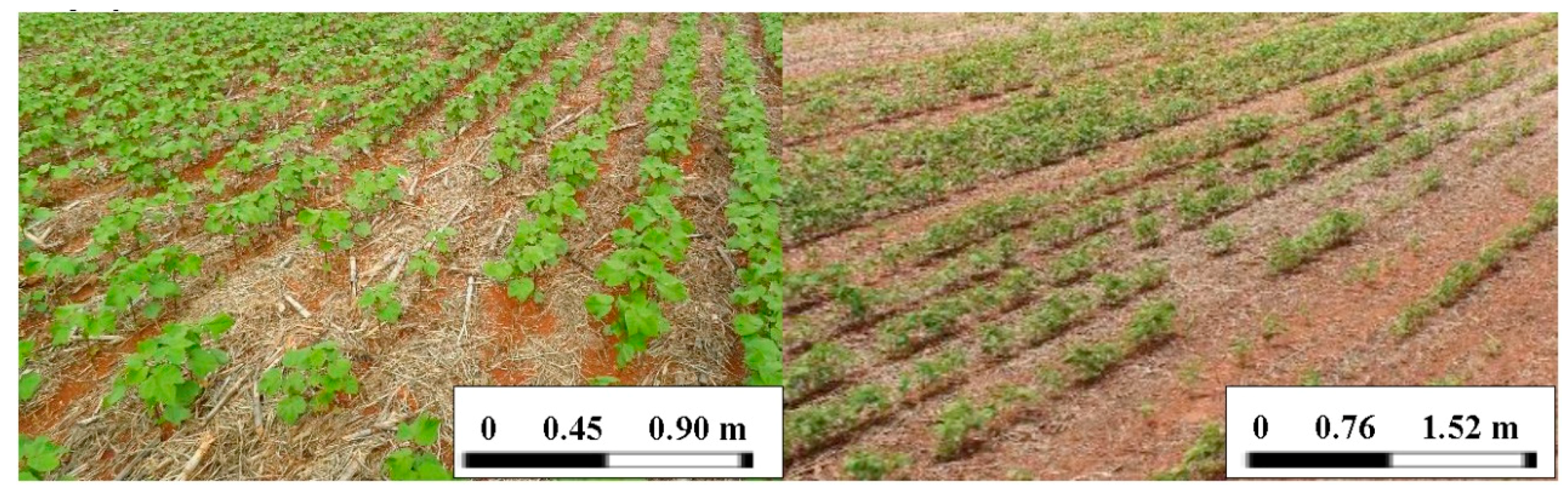
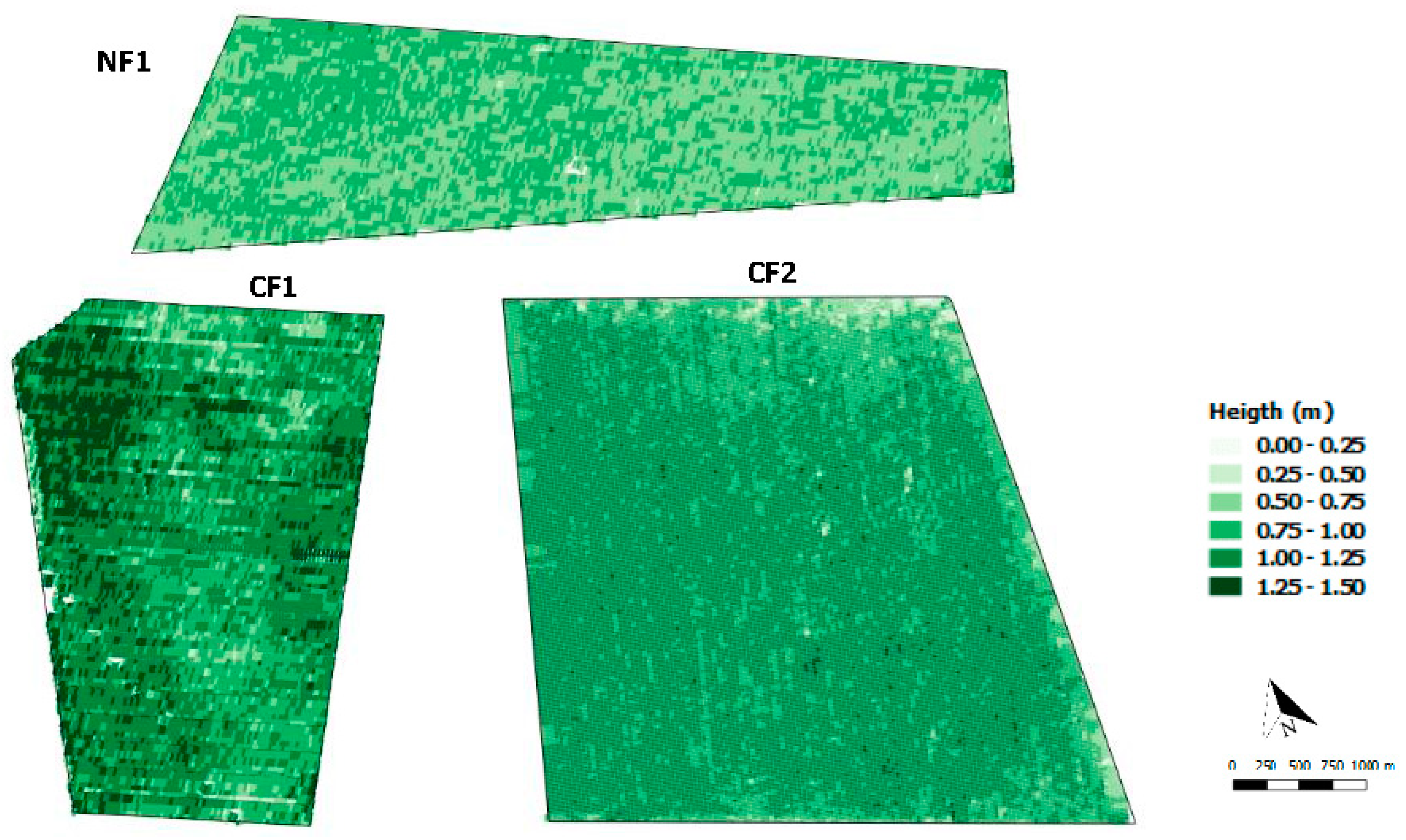
Figure 1. Approximate view from each sensor position and mounting points in the high clearance vehicle used to move the sensors through the field. Pictures from 2014/2015 crop season of narrow row cotton cultivated in a sandy loam Quartzipsamment in Mato Grosso state.
Agriculture 08 00101 g001
Figure 2. Variable rate application of plant growth regulator in narrow-row cotton using an electronic flow controller.
Agriculture 08 00101 g002
Figure 3. Uneven crop emergence and short scale variability at BBCH 51 in field NF1 during the 2013/2014 crop season and BBCH 51 in field CF3 during the 2014/2015 crop season.
Agriculture 08 00101 g003
Figure 4. Relation of crop aboveground fresh biomass and crop height in five crop stages (BBCH) for cotton cultivated in two systems: narrow row (NF1) and conventional row spacing (CF1).
Agriculture 08 00101 g004
Figure 5. Sensor performance to predict crop parameters: dry biomass (Dry B.), fresh biomass (Fresh B.), height of top five nodes (H. Five), crop height (Height) and height-to-node ratio (HNR) with three crop sensors: OPS1: N-Sensor™ ALS; OPS2: Crop Circle ACS 430; US2: HC-SR04; for cotton cultivated in two systems: narrow row (NF2) and conventional row spacing (CF2 and CF3).
Agriculture 08 00101 g005
Figure 6. Frequency distribution of crop height in field NF2 under fixed-rate and variable-rate application of plant growth regulators.
Agriculture 08 00101 g006
Figure 7. Spatial distribution of crop height in five phenological stages of narrow-row cotton in field NF2.
Agriculture 08 00101 g007
Figure 8. Frequency distribution of crop height in field CF3 under fixed rate and variable rate application of plant growth regulators.
Agriculture 08 00101 g008
Figure 9. Spatial distribution of crop height in five phenological stages of conventional row spacing cotton in field CF3.
Agriculture 08 00101 g009
Figure 10. Spatial distribution of applied plant growth regulators and cottonseed yield in narrow row cotton in field NF2.
Agriculture 08 00101 g010
Figure 11. Spatial distribution of applied plant growth regulators and cottonseed yield in conventional row spacing cotton in field CF3.
Agriculture 08 00101 g011
Table 1. Field and crop characteristics of areas used for data collection.
Field *StateCrop SeasonArea (ha)Row Spacing (m)VarietyEmergence DateSeed Density (Seed ha−1)
CF1GO2013/201493.80.80FM 975 WS8 January 2014100,000
NF1GO2013/201488.50.45FM 975 WS23 January 2014190,000
CF2MT2014/2015139.70.76DP 1243 B2RF7 January 201595,000
NF2MT2014/2015203.40.45TMG 81 WS22 January 2015205,000
CF3MT2014/2015142.30.76TMG 81 WS17 January 2015100,000
* CF: conventional row spacing cotton; NF: narrow row cotton; GO: Goias State; MT: Mato Grosso State.
Table 2. Technical specifications of crop canopy optical sensors evaluated in cotton fields.
Sensor SystemOPS1OPS2
ModelN-Sensor ALSCrop Circle ACS 430
Light sourceXenonPolychromatic modulated LED
Spectral bands730 nm (RedEdge)
760 nm (NIR)
670 nm (RED)
730 nm (RedEdge)
780 nm (NIR)
Vegetation index100 × ( ln ( R 760 ) ln ( R 730 ) ) ( R 780 R 730 R 780 + R 730 )
Acquisition frequency1 Hz5 Hz
Mounting height2.0–4.0 m0.6–1.2 m
Field of view40°–55°45/10°
Sensor footprint2.0–4.0 m0.5–1.0 m
Table 3. Technical specifications of crop canopy ultrasonic sensors evaluated in cotton fields.
Sensor SystemUS1US2
ModelPolaroid 6500HC-SR04
Working frequency49.4 kHz40.0 kHz
Acquisition frequency1 Hz5 Hz
Mounting height0.6–1.2 m0.6–1.2 m
Field of view30°20°
Sensor footprint0.3–0.6 m0.2–0.4 m
Table 4. Performance of crop sensors measured by coefficient of determination and root-mean-squared error to predict crop height and aboveground biomass in five crop stages.
Crop ParameterFieldSensorBBCH *
5161718195
HeightNF1OPS10.70 (0.02)0.64 (0.03)0.68 (0.05)0.62 (0.03)0.67 (0.04)
OPS20.18 (0.03)0.38 (0.04)0.04 (0.08)0.37 (0.04)0.23 (0.06)
US10.02 (0.04)0.11 (0.05)0.00 (0.08)0.29 (0.05)
CF1OPS10.83 (0.02)0.94 (0.03)0.90 (0.07)0.32 (0.12)0.55 (0.10)
OPS2 0.52 (0.08)0.80 (0.10)0.11 (0.13)0.48 (0.11)
US10.01 (0.05)0.75 (0.06)0.85 (0.08)0.56 (0.09)
Fresh BiomassNF1OPS10.78 (0.50)0.68 (1.12)0.54 (2.73)0.27 (2.75)0.64 (3.49)
OPS20.43 (0.81)0.56 (1.27)0.02 (4.00)0.28 (2.74)0.31 (4.81)
US10.04 (1.05)0.21 (1.71)0.00 (4.04)0.00 (2.90)
CF1OPS10.67 (0.48)0.96 (0.76)0.90 (2.77)0.17 (5.45)0.55 (5.08)
OPS2 0.57 (2.45)0.80 (3.98)0.14 (5.55)0.48 (5.44)
US10.01 (0.71)0.70 (1.94)0.71 (4.82)0.39 (4.67)
* BBCH: crop stage according to BBCH scale for cotton; OPS1: N-Sensor™ ALS; OPS2: Crop Circle ACS 430; US1: Polaroid 6500; First value in each cell: coefficient of determination (R2), value in parenthesis: root-mean-squared error (RMSE).
Table 5. Performance of crop sensors measured by coefficient of determination and root-mean-squared error to predict crop parameters of cotton cultivated in conventional and narrow row spacing.
FieldSensor *Dry B.Fresh B.H. FiveHeightHNR
CF2OPS10.46 (0.15)0.66 (0.31)0.38 (0.02)0.77 (0.07)0.50 (0.51)
OPS20.65 (0.14)0.74 (0.29)0.51 (0.02)0.81 (0.07)0.69 (0.47)
US20.52 (0.15)0.73 (0.29)0.41 (0.02)0.84 (0.06)0.61 (0.49)
CF3OPS10.65 (0.14)0.81 (0.21)0.50 (0.02)0.72 (0.06)0.44 (0.37)
OPS20.58 (0.14)0.71 (0.24)0.38 (0.02)0.55 (0.07)0.37 (0.36)
US20.61 (0.14)0.75 (0.23)0.53 (0.02)0.78 (0.05)0.43 (0.37)
NF2OPS10.71 (0.19)0.85 (0.33)0.66 (0.04)0.82 (0.08)0.73 (0.50)
OPS20.74 (0.19)0.91 (0.27)0.80 (0.03)0.89 (0.07)0.78 (0.47)
US20.71 (0.19)0.90 (0.27)0.79 (0.03)0.92 (0.06)0.81 (0.45)
* OPS1: N-Sensor™ ALS; OPS2: Crop Circle ACS 430; US2: HC-SR04; Dry B.: dry biomass; Fresh B.: fresh biomass; H. Five: height of top five nodes; Height: hand measured crop height; HNR: height-to-node ratio; First value in each cell: coefficient of determination (R2), value in parenthesis: root-mean-squared error (RMSE).
Table 6. Input savings with variable rate application of plant growth regulators and fruit ripener in cotton variety TMG 81 WS in conventional and narrow row fields.
FieldApplicationBBCHProductAverage Rate (L ha−1)
Fixed RateVariable Rate
NF21st PGR51PIX HC0.0300.026
2nd PGR61PIX HC0.0500.043
3rd PGR71PIX HC0.0800.069
4th PGR76PIX HC0.1200.104
5th PGR81PIX HC0.1500.131
Defoliant98DROPP ULTRA0.4000.312
Boll Opener98FINISH2.0001.560
CF31st PGR71PIX HC0.0500.046
2nd PGR76PIX HC0.0800.053
3rd PGR81PIX HC0.1200.080
Defoliant98DROPP ULTRA0.5000.458
Boll Opener98FINISH2.5002.292

