Automatic Identification of Center Pivot Irrigation Systems from Landsat Images Using Convolutional Neural Networks

Abstract

Being hailed as the greatest mechanical innovation in agriculture since the replacement of draft animals by the tractor, center pivot irrigation systems irrigate crops with a significant reduction in both labor and water needs compared to traditional irrigation methods, such as flood irrigation. In the last few decades, the deployment of center pivot irrigation systems has increased dramatically throughout the United States. Monitoring the installment and operation of the center pivot systems can help: (i) Water resource management agencies to objectively assess water consumption and properly allocate water resources, (ii) Agro-businesses to locate potential customers, and (iii) Researchers to investigate land use change. However, few studies have been carried out on the automatic identification and location of center pivot irrigation systems from satellite images. Growing rapidly in recent years, machine learning techniques have been widely applied on image recognition, and they provide a possible solution for identification of center pivot systems. In this study, a Convolutional Neural Networks (CNNs) approach was proposed for identification of center pivot irrigation systems. CNNs with different structures were constructed and compared for the task. A sampling approach was presented for training data augmentation. The CNN with the best performance and less training time was used in the testing area. A variance-based approach was proposed to further locate the center of each center pivot system. The experiment was applied to a 30-m resolution Landsat image, covering an area of 20,000 km² in North Colorado. A precision of 95.85% and a recall of 93.33% of the identification results indicated that the proposed approach performed well in the center pivot irrigation systems identification task.

1. Introduction

Although 94% of irrigation in the world is surface irrigation [1], sprinkler irrigation accounts for about 63% of the irrigated areas in the United States (2012) [2]. The major reason for this large percentage of sprinkler irrigation in the United States is the popularity of the center pivot irrigation system. Among all sprinkler systems, including center pivot, turf, wheel-line and hand-line, orchard and micro sprinkler ones, the center pivot irrigation system (CPIS) is the most widely employed sprinkler irrigation system, and it covers 75% of the sprinkler irrigated land in the United States [3].

Center pivot is based in concept, on a water well located in the center of an area (usually a one-quarter section, or 64.75 hectares), with a linear system of pipes and sprinklers carried on large wheels in a circle around the well. This irrigation innovation has been widely employed in the United States, especially within the states of Colorado, Nebraska, Kansas, and others, since the early 1950s [4].

Center pivot irrigation system has had an impact on the environment due to its extensive deployment and huge consumption of water and energy. Compared to surface irrigation, which distributes water by gravity, a center pivot irrigation system requires expensive hydraulic pressure techniques and consumes huge energy. On average, in Nebraska, an estimated 496 L of diesel fuel (or the equivalent) per hectare-year is consumed to apply over 3,806,511 L of water per hectare-year [5]. Moreover, the increased use of water by center pivot irrigation systems has also been considered as a threat to the local environment, particularly ground water balance. According to Brown, by the early 1980s, center pivot irrigation systems were widely used in Nebraska, where they allowed farmers to irrigate crops more regularly. This large ground-covering sprinkler system significantly increased crop yields and quickly drained the Ogallala Aquifer, which delivers freshwater for roughly one-fifth of the crops in the United States [6]. Farmers were at risk of losing their livelihood. The situation in Kansas is even worse than in Nebraska, where a report from The National Aeronautics and Space Administration(NASA) shows that about 30 percent of the water once stored beneath Kansas is already gone, and another 40 percent will be gone within 50 years if current irrigation trends continue [7]. Problems occurred in the Ogallala Aquifer are now being noticed and alternative farming methods are being adapted. Studies and methods on improving the water and energy use efficiency of center pivot irrigation systems, have been proposed during the past decades [8,9,10]. On the other hand, information about the distribution and development of center pivot irrigation systems is very important when one intends to study water availability or growth potential of irrigated areas for a specific site, due to the increasing concern about drinking water worldwide and nationally [11].

Along with the steady increase in numbers and profound impacts on the environment and rural landscape of center pivot irrigation systems, several studies have been carried out to monitor the increase of these systems. The first program of center-pivot monitoring dates to 1973, where it was proposed by the NASA University Affairs program. Several principal investigators and many students were involved in the project, in the early 1970s. However, only the state of Nebraska had consistently employed remote sensing images to monitor the diffusion of center pivot irrigation systems. To investigate the long-term inventory of Nebraska center pivots, Carlson collected Landsat TM Band-3 images from 1972 to 1986 in Nebraska to visually interpret center pivot systems, where a near ten-fold increase over 14 years was observed [12]. Instead of using satellite images, Seth used aerial images in Custer County, Nebraska, USA, from 2003 to 2010, to manually digitize center pivot systems. It showed that there was a large increase of center pivots from 2003 to 2010 as well, with a 39% increase over the seven-year period [4]. Using the same approach with Carlson, Schmidt identified 2485 center pivots in the state of Minas Gerais, Brazil, by visual interpretation through LANDSAT images [11]. Similarly, Ferreira utilized Red, Green and Blue (RGB) color composite images acquired through the satellite CBERS2-2B/CCD in the State of Minas Gerais, for visual identification of center pivots. There were 3781 center pivot systems identified, and the authors confirmed the reliability of remote sensing images in mapping irrigated areas [13]. In the Distrito Federal region, the method of visual interpretation on images was also applied by Sanoto interpret Landsat5-TM images in 1992 and 2002, for a survey of the areas irrigated by center pivots [14]. Through the review of existing literature on center pivots monitoring, the basic methodology applied by researchers is based on visual interpretation of occurrences of the characteristic circular features. Little effort has been made for automatic identification of center pivot irrigation systems based on remote sensing images. Although the approach based on visual interpretation is relatively simple, the process of identification and digitizing can be very time and labor consuming, if the approach is applied to a wide range of areas for yearly identification.

For the task of basic shape detection, methods based on Hough Transform (HT) have been proposed, like Standard HT, Fast HT [15], and Randomized HT [16]. It achieves this by determining the specific values of parameters, which characterize these shapes [17]. HT first transforms each point of feature into a parameter space, then a voting procedure is used on the parameter space to find objects. For example, in the case of circles, the parameter space is three dimensional (i.e., the radius, and the x and y coordinates of the center). The use of the HT to detect circles was first outlined by Duda and Hart [18]. Studies on using HT for object extraction have been carried out for a long time. For example, Hu used a modified HT method to directly detect road stripes [19]. Vozikisa compared the advantages and disadvantages of using HT for building extraction [20]. Zhang proposed an HT based approach for automatic oil tank detection on satellite images [21]. Using SAR and optical images, Wang applied an improved HT method for circular oil tanks [22]. Nevertheless, due to increased complexity with increased parameter space dimensionality, it is practically of use only for simple cases. Moreover, HT can find complete circles like oil tanks, whilst it is hard for HT to handle situations where the circle is not complete, such as a half circle or a circle with the rectangular corner.

In recent years, deep learning has become the new state-of-the-art solution for prediction and classification tasks [23]. It has been intensively used in different agriculture-related applications due to its great success, such as in plant recognition [24], corn yield estimation [25], vegetation quality assessment [26], soil moisture content [27], and fruit counting [28]. Deep learning is a branch of machine learning techniques that refers to multi-layered interconnected neural networks, which consist of various components (e.g., convolutions, pooling layers, fully connected layers, activation functions, etc.), depending on the network architecture used (i.e., Convolutional Neural Networks, Recurrent Neural Networks, Recursive Neural Networks). Convolutional Neural Networks (CNNs) are a feed forward neural network generally used for image recognition and object classification, such as scene labeling [29], face recognition [30], sentence modeling [31], and handwritten character classification [32]. A Recurrent Neural Network (RNN) is a class of artificial neural networks, where connections between nodes form a directed graph along a sequence [33]. Different from feed forward neural networks like CNNs, RNN is fed data then it outputs a result back into itself and continues to do this. Breakthroughs like Long Short-Term Memory (LSTM) make it able to memorize previous inputs and find patterns across time. It is used for sequential inputs, where the time factor is the main differentiating factor between the elements of the sequence. CNNs considers only the current input, whilst RNNs consider both the current and past inputs. CNNs are designed to recognize images, whilst RNNs are ideal for recognizing sequences, for example, a speech signal [34] or a text [35]. A Recursive Neural Network is more like a hierarchical network, where there is no time aspect to the input sequence, but the input must be processed hierarchically in a tree fashion [36]. The satisfying performance of CNN on object detection and classification shows promise in the task of center pivot irrigation system identification.

In this paper, a Convolutional Neural Networks (CNNs) approach for identification and location of center pivot irrigation systems using remote sensing images is presented. The main innovations of this study are:

• Automation of identifying and locating of CPIS at high accuracy from Landsat images. Traditional method for identifying and locating CPIS is mostly based on visual interpretation, which is labor intensive and prone to errors. The approach described in this paper largely automates the task of identifying and locating CPIS from remotely sensed images.
• Using CNNs to train a classification model for center pivot irrigation systems. By learning features from training data, CNNs can easily achieve high accuracy in identifying center pivot irrigation systems from remotely-sensed images. Seed images are clipped from remote sensing data, and then are sampled as training data to train the classifier. Given that the performance of CNNs relies heavily on large-scale learning samples, a sampling strategy is presented for selecting a large volume of training samples from remote sensing images. A set of candidate center points for each center pivot irrigation system are identified using the classifier. Three CNNs with different structures were compared for the task.
• A variance-based approach for locating the center of center pivots. CNNs can identify images which are of high possibility to be the center pivot irrigation systems. However, it is a challenge for CNNs to accurately locate the center of center pivots. Therefore, a center locating approach based on variance value is introduced to find the center of each center pivot system.

The rest of the paper is organized as follows. Convolutional neural networks are introduced in Section 2. Experimental data are described in Section 3. Three CNNs with different structures for the identification task, and the related approach and experiments are described in Section 4. To validate the availability of the classification model, the model trained on data from 2011 was applied for center pivot detection on images collected in 1986 and 2000, respectively. The derived results and comparisons of the three CNNs are presented in Section 5. Discussion is presented in Section 6. Finally, Section 7 concludes this work and discusses future work.

2. Convolutional Neural Networks

With the rapid development of computer vision and image analytics in recent years, machine learning techniques, especially neural networks, have achieved great improvement. As the earliest type of neural networks, artificial neural networks (ANNs) are structured by fully connected layers. All neurons from the previous layer are connected to the neurons of the following layer, leading to a tremendous volume of training data and computational resources in the task of 2D image classification. Furthermore, by giving each neuron all pixels as input, ANNs is highly dependent on object locations, which also leads to the low performance of ANNs. CNNs [37], as an advanced development of ANNs, are characterized by local connectivity between layers and are a multilayer neural network composed of different types of layers. Each neuron in the convolutional layer can be considered as a weight matrix. The weight matrix is connected to a local region of the image. By sliding weight matrices over the image, features of the image are extracted and fed into the next layer. This process transforms the image into another form called a feature map. It should be noted that the weight matrix of each neuron is shared for the whole image. Then a pooling layer is usually followed by a convolutional layer, the pooling layer subsamples the result of the convolution operation by extracting the maximum value of a feature map. The fully connected layer is located at the end of the CNNs and is tasked with the classification or regression task. The strategy of local connectivity of CNNs largely decreases the number of weights that need to be computed in layers and reduces the amount of training data.

A pioneering 7-level convolutional network named LeNet-5, developed by LeCun in 1998, was applied for handwriting recognition [38]. LeNet-5 consisted of two convolutional layers, with each followed by a sigmoid or tanh nonlinearity operator, two average pooling layers, and three fully connected layers. LeNet was constrained by the availability of computing resources and had a poor ability for higher resolution images. In recent years, more complex structures and deeper networks have been developed. The AlexNet [39] proposed during the ImageNet challenge in 2012, marked a significant improvement in application of CNNs for image classification. The network had a very similar architecture to LeNet, but deeper. The network was made up of five convolutional layers, three max pooling layers, two drop out layers, and three fully connected layers. Rectified Linear Unit (ReLU) was used for the nonlinearity functions after the convolutional layer to decrease training time. Dropout layer was implemented to combat the challenge of over fitting of the training data. AlexNet significantly outperformed all the prior competitors and won the challenge by reducing the top-5 error to 15.3%. Techniques used in AlexNet, such as dropout layers, max pooling, and ReLU nonlinearity, are still used today. A network deeper, but simpler than AlexNet, called VGGNet, was developed by Simonyan and Zisserman in 2014. VGGNet consisted of 16 convolutional layers and maintained a very uniform architecture by using 3 × 3 sized filters in all convolutional layers. With two 3 × 3 layers stacked, each neuron had a receptive field of 5 × 5. Number of parameters in two stacked 3 × 3 layers was 18, whilst the 5 × 5 layer had a number of 25, which led to the decrease in the number of parameters. With two convolutional layers, two ReLU layers can be attached instead of one. Therefore, the introduction of VGGNet suggested some standards, i.e., all filters should have size of 3 × 3, and the number of filters should be doubled after each max pooling layer. Additionally, GoogleNet [40] was presented in 2014 and had a significantly different architecture compared to CNNs, built with general approaches of simply stacking convolutional and pooling layers on top of each other in a sequence. GoogleNet was implemented with a novel element, named an inception module. The inception module had parallel paths with different receptive field sizes and operations. The network was quite deep using nine inception modules in the whole architecture, with over 100 layers in total. The authors of the paper emphasized that this structure placed notable consideration on memory and power usage.

In this study, three different CNNs following the structures of LeNet, AlexNet, and VGGNet, respectively, with a bit of modification, were trained for CPIS identification. Since the image objects of this study were regularly shaped objects at low spatial resolution, and that GoogleNet requires considerable computational resources, the GoogleNet structure was not considered in this study.

3. Data

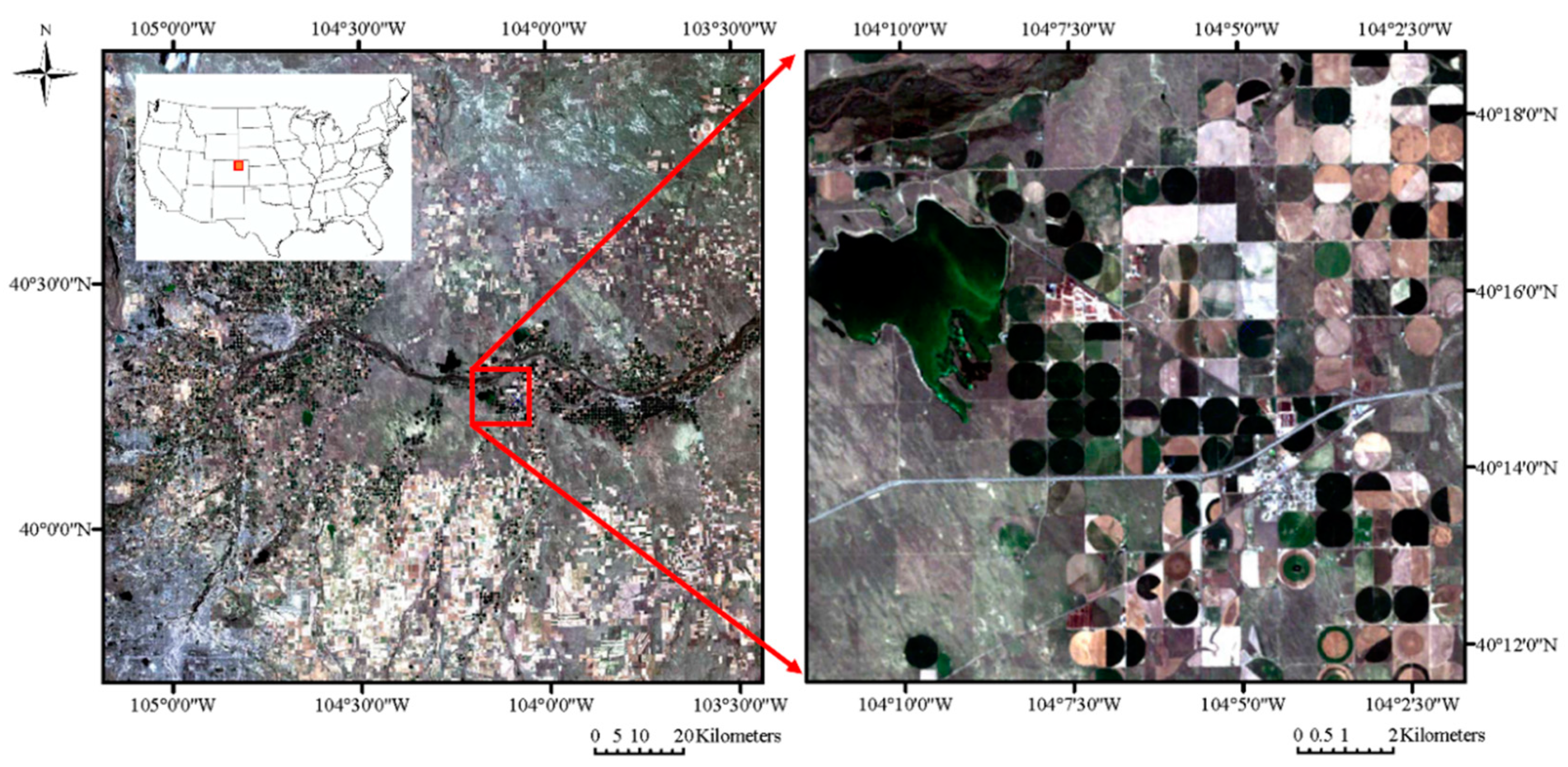
Landsat data and Crop Data Layer (CDL) were used in the study. The Landsat 5-TM level 1 product with resolution of 30 m was downloaded from the website of the U.S. Geological Survey [41]. Considering the wide distribution of CPIS in the Great Plains of the United States, images with coverage area of 20,000 km² in the north-east of Colorado State were clipped from Landsat data. Band 1 (blue), Band 2 (green), and Band 3 (red) of Landsat TM data, were used as input to train the model. 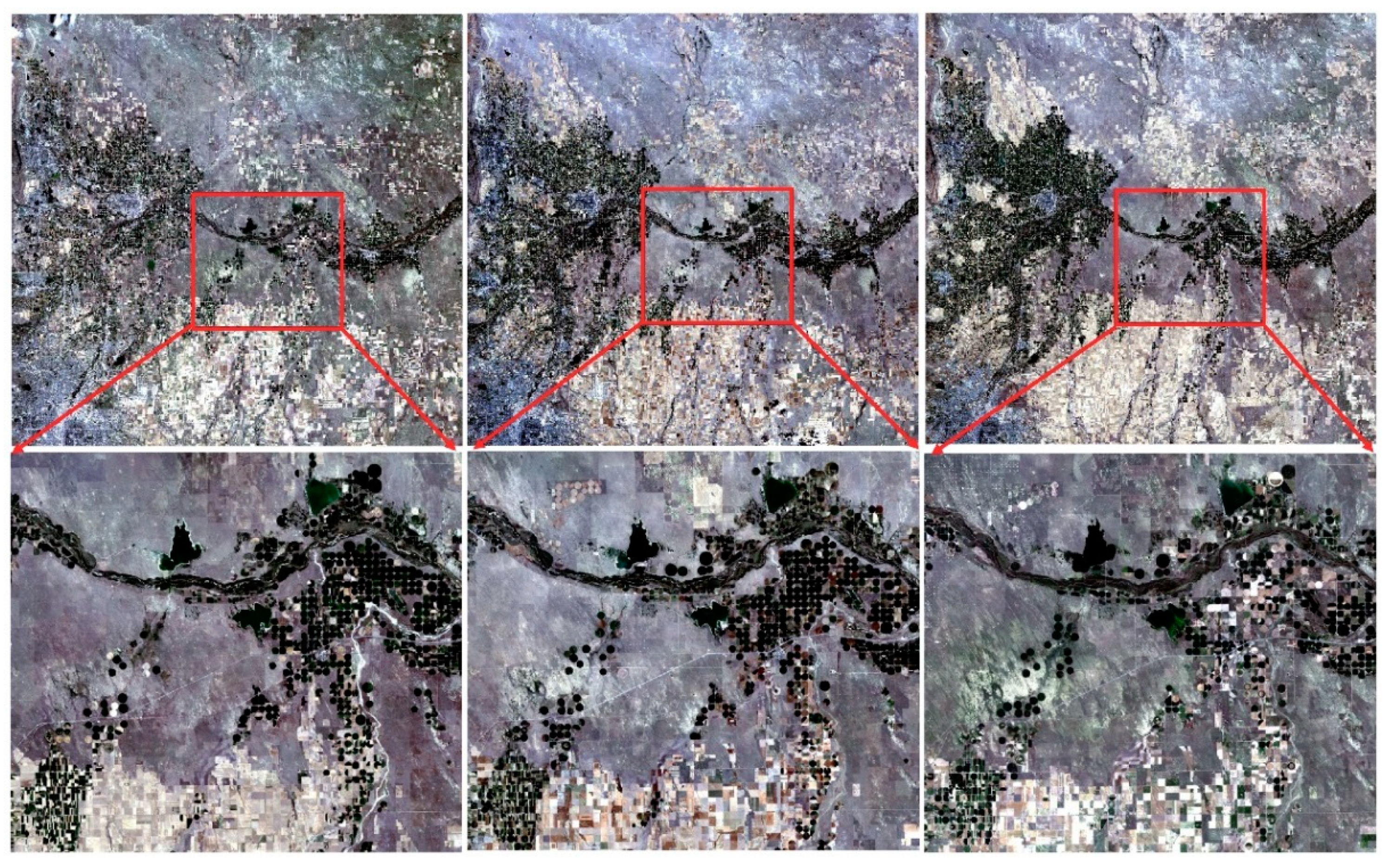The image is shown in Figure 1. To validate the described approach, Landsat 5-TM images of the same area from the years 1986 and 2000, were downloaded and used for comparison. Images are shown in Figure 2.

CDL is produced by the National Agricultural Statistics Service (NASS) of the US Department of Agriculture (USDA). It provides crop cover categories in 30 m resolution, with accuracies ranging from 85% to 95% [42]. With regards to high accuracy of land use classification, CDL is incorporated to screen non-cropland areas in Landsat data. CDL data is freely available through the CropScape web service system [43].

Though there exists little difference in planting time from south to north in the United States, planting in the United States usually begins in April, and crops grown mature in early fall, then the harvest finishes by the end of November. With crops grown maturing in late July-early August, CPIS can be identified on Landsat imagery due to its distinctive shape of a circle. Therefore, the Landsat-5 TM image on 19 July 2011, with less cloud cover, was selected as experimental data.

4. CNNs-Based Center Pivot Irrigation Systems Identification

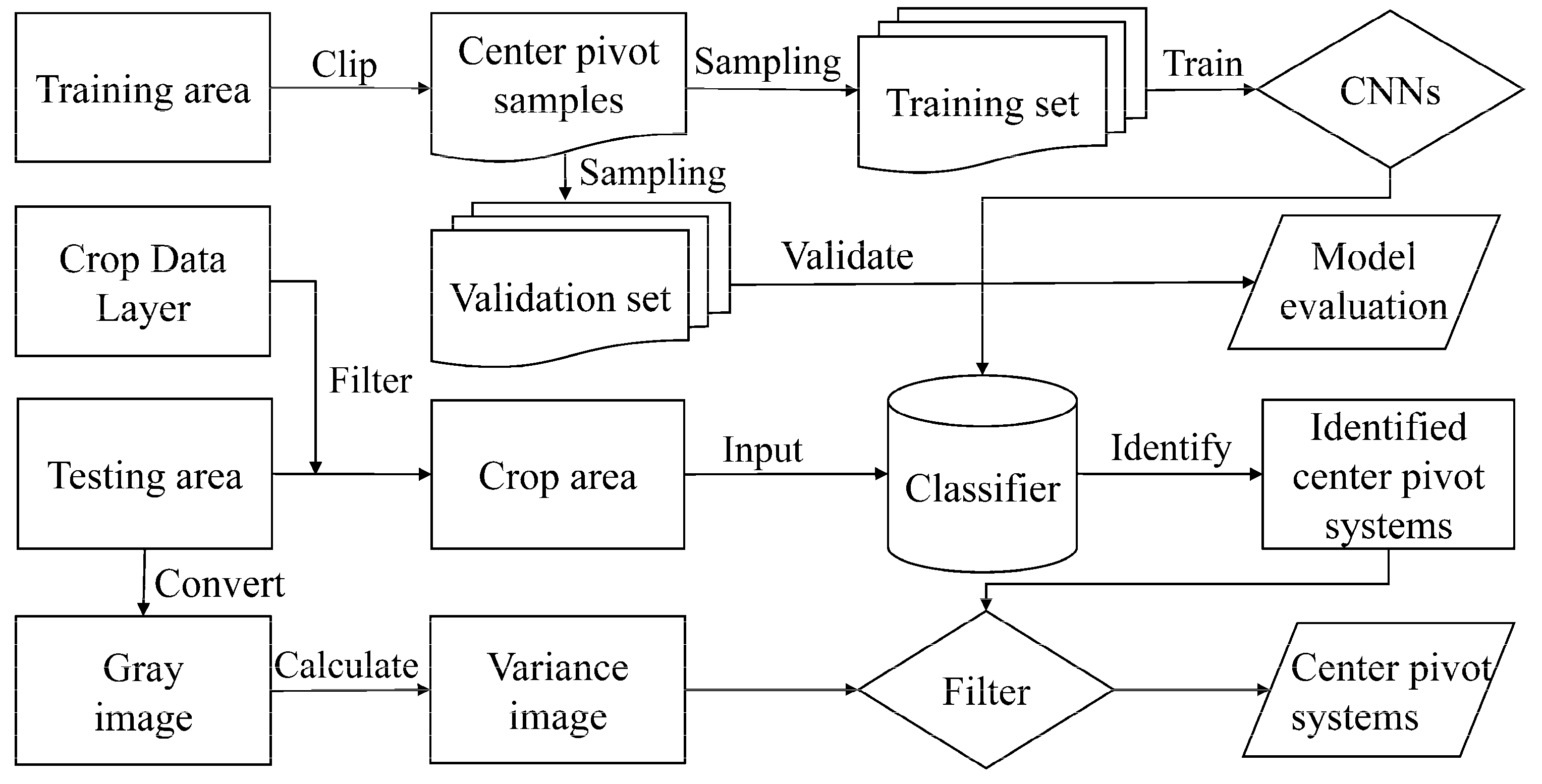
The framework of our approach is shown in Figure 3.

The major work consists of two parts: A CNN classifier adopted for CPIS identification, and a variance-based approach for accurately locating the center of a CPIS. As shown in Figure 1, shapes and colors vary significantly between different center pivot systems as a result of the variation of cultivation and irrigation, and most of the center pivot systems have a similar covering area (usually a one-quarter section, or 64.75 hectares) [12]. Therefore, a set of representative center pivot irrigation systems images were clipped using a fixed size window from the training area. Then a sampling strategy for enlarging the volume of training data was used for better identification performance. We evaluated the model with a validation set. To locate the center of center pivot systems identified by the classifier, CDL was firstly used to filter out non-cropland areas, such as open waters, developed spaces and forests, from the Landsat images. Then the trained classifier classified filtered data to get clusters of CPIS. A variance image was produced by our approach, using a gray image converted from a true color image. Finally, the variance image is combined with CPIS clusters for locating CPIS with high accuracy.

4.1. Data Preprocessing

Three visible channels (band 3—red, band 2—green, band 1—blue) from Landsat 5-TM were used as the main input data for identification. Then a true color image was composited from the three visible channels, for manually labeling the center pivot systems. An area covering 2644 km² was selected as the training area, from which training and validation datasets were clipped. In the training area, nearly 300 CPISs with different colors and internal shapes were visually marked. The center pixels of each CPIS were marked with the value of 1 in a new raster layer, whilst the non-center pixels were assigned the value of 0. It needs to be noted that values in the new raster were only used to distinguish if the pixel was in a CPIS or not, not for training the model. A clip and sampling strategy was applied in the next step, to construct the training data.

A test image covering an area of 21,000 km² was used for testing after the training process. Land covers for open waters, developed spaces, grassland/pastures, and forests were filtered out using CDL, which can largely decrease the input for the identification task.

4.2. Training Data

This section describes the construction of the training data. To identify if an image is a CPIS or not, images depicting CPISs and non-CPISs need to be clipped from the training area and put into the model.

A window with size of 34 × 34 was used to clip both CPISs images and non-CPISs. The reason to use a window of 34 × 34 pixels in size, was because almost all CPISs have a circular shape with a similar radium, covering 27 × 27 pixels in Landsat TM images. We carefully decided on the size of the training and validation images, for its effect on performance of the model. If the size was too large, more than one CPIS may be observed in a single image, which may lead to noise features being extracted by the model. Conversely, if the size is too small, the distinguishable characteristics of CPISs may fail to be captured. The size of 34 × 34 pixels used in this study was determined to balance between finding a CPIS and reducing the risk of misclassification. For each pixel identified as the center of a CPIS (which has a value of one in the new raster layer), a window with size of 34 × 34 covering the CPIS was used for the CPIS image from the true color composite image. For pixels identified as the non-center of center pivot systems, an area of 34 × 34 pixels was also clipped by the window into the training data, for non-CPIS identification.

All training data were labeled, as either center pivot systems or non-center pivot systems. However, data labeled as center pivot systems were much less than data labeled as non-center pivot systems. To overcome the limited number of samples, image transformations, such as flipping, rotating, and cropping have been proposed [44,45]. In this work, a sampling approach was proposed to augment the number of training samples. This approach is based on the idea that images with centers that are slightly off the centers of CPISs, should also be considered as samples of CPISs. The approach is presented in Figure 4.

For each center pivot system area, a window with 34 × 34 pixels in size was used to slide over the original image horizontally and vertically in both directions, on one pixel at a time. The original image within the window is clipped out as a training image. For example, in Figure 4b, the center image is zero off the center. The upper-right image is two pixels off the center, in the upward and rightward directions. With this strategy, the number of training images was multiplied by 25 times. Then rotations were applied to all images to further expand the available training images. The number of CPISs was significantly increased through this process. Since there were still many more non-CPIS samples than CPIS samples, non-CPISs was randomly clipped from the training area to a number roughly similar to the number of CPIS samples.

4.3. Architectures of CNNs

Three CNNs with their network structure based on LeNet, AlexNet, and VGGNet, respectively, were used for comparison in this study. The initial input of each CNN was an RGB image 34 × 34 × 3 pixels in size. RGB values were normalized for each color. The output was a binary classification of center pivot systems and non-center pivot systems. Architecture of each network is detailed below.

4.3.1. Architecture Based on LeNet

This network was based on the structure of LeNet. The network consisted of two convolutional layers, two max pooling layers, and two fully connected layers. The first convolutional layer utilized 20 filters with a size of 3 × 3 × 3, followed by a rectified linear operator (ReLU), and a max pooling layer taking the maximal value of 3 × 3 regions with two-pixel strides. Output of the first max pooling layer is a 17 × 17 × 20 blob. Then the blob was processed by the second convolutional layer, containing 50 filters with size of 20 × 3 × 3. ReLU was also used after the second convolutional layer. A max pooling layer was used again with the same hyper parameters as before. Feature maps extracted by the previous layers were transformed into a simple vector in the flattened layer. Finally, two fully connected layers with neurons of 500 and 2 were connected at the end of the network, followed by a ReLU and soft-max operator, respectively. The soft-max operator assigned a probability for each class. Architecture is shown in Figure 5.

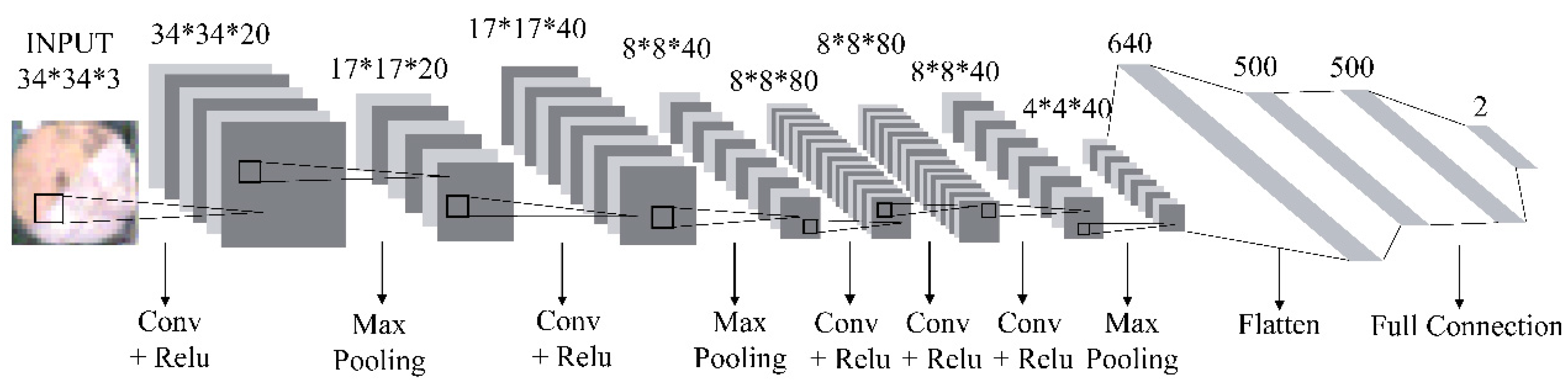
4.3.2. Architecture Based on AlexNet

Structure of AlexNet is similar to LeNet, but deeper with more layers. This network consisted of five convolutional layers each followed by a ReLU operator, three max pooling layers, and three fully connected layers. Twenty filters with size of 3 × 10 × 10 were used in the first convolutional layer. Number of filters was doubled to 40 in the second convolutional layer with size of 20 × 5 × 5. Each convolutional layer was followed by a max pooling layer with pool size of 2 × 2. The image was transformed to an 8 × 8 × 40 feature map, after the first two max pooling layers. The 8 × 8 × 40 output of previous layers was then processed by three connected convolutional layers. The third convolutional layer contained 80 filters with size of 8 × 8 × 40, followed by a ReLU layer. The fourth convolutional layer had 80 filters with size of 8 × 8 × 80. Again, this was followed by a ReLU layer. A configuration of 40 filters with size of 8 × 8 × 80 was used in the last convolutional layer. A max pooling layer taking the maximal value of 2 × 2 regions with two pixel strides was applied on the final extracted feature map. Finally, 4 × 4 × 40 features were flattened to a vector and fed to three fully connected layers. The first two fully connected layers had 500 neurons, the final fully connected layer had 2 neurons, which stand for center pivot systems and non-center pivot systems. Figure 6 shows the architecture based on AlexNet.

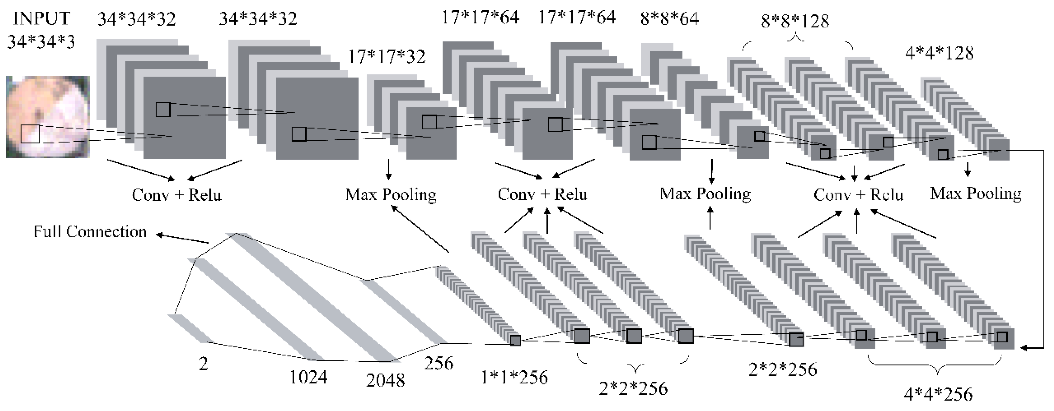
4.3.3. Architecture Based on VGGNet

This network is deeper but maintains its simplicity based on the idea of VGGNet. The network consisted of thirteen convolutional layers, five max pooling layers, and three fully connected layers. The whole structure of the network can be viewed as five stages. Each stage had a similar layer stack arrangement. The first two stages had two convolutional layers and one max pooling layer. Three convolutional layers and one max pooling layer were contained in the next three stages. Number of filters in convolutional layers in the next stage were doubled after the previous stage, from 32 to 256. Convolutional layers used in the fifth stage were the same as the fourth stage. Filters with height and width set to 3 and with a stride of 1, were applied in all convolutional layers. All max pooling layers were arranged to have 2 × 2 filters with a stride of 2. Each convolutional layer was followed by a ReLU operator. Then, 256 features were extracted through the five stages. Features were then flattened and fed to a three fully connected layer stack. To limit the risk of overfitting, two dropout layers with a dropout ratio of 0.5 were applied after the fully connected layers. The soft-max operator was also used in the last fully connected layer to assign a probability to each class. Figure 7 shows the architecture of CNNs based on the VGGNet structure.

4.4. Model Training and Validation

The training data were fed into the three networks described above to train the networks. It should be noted that training data were divided by a 9:1 split between training set and validation set. The validation set was used for validation after the training process. The initial learning rates were set to 0.001. The loss of the VGGNet-based network did not decrease in the beginning of the training with a 0.001 learning rate. A common strategy is to decrease the learning rate, when the loss stagnates. Therefore, the learning rate of the VGGNet-based network was set to 0.0001. All experiments were run for 20 iterations using the Adam optimization.

4.5. Variance Based Approach for Center Locating

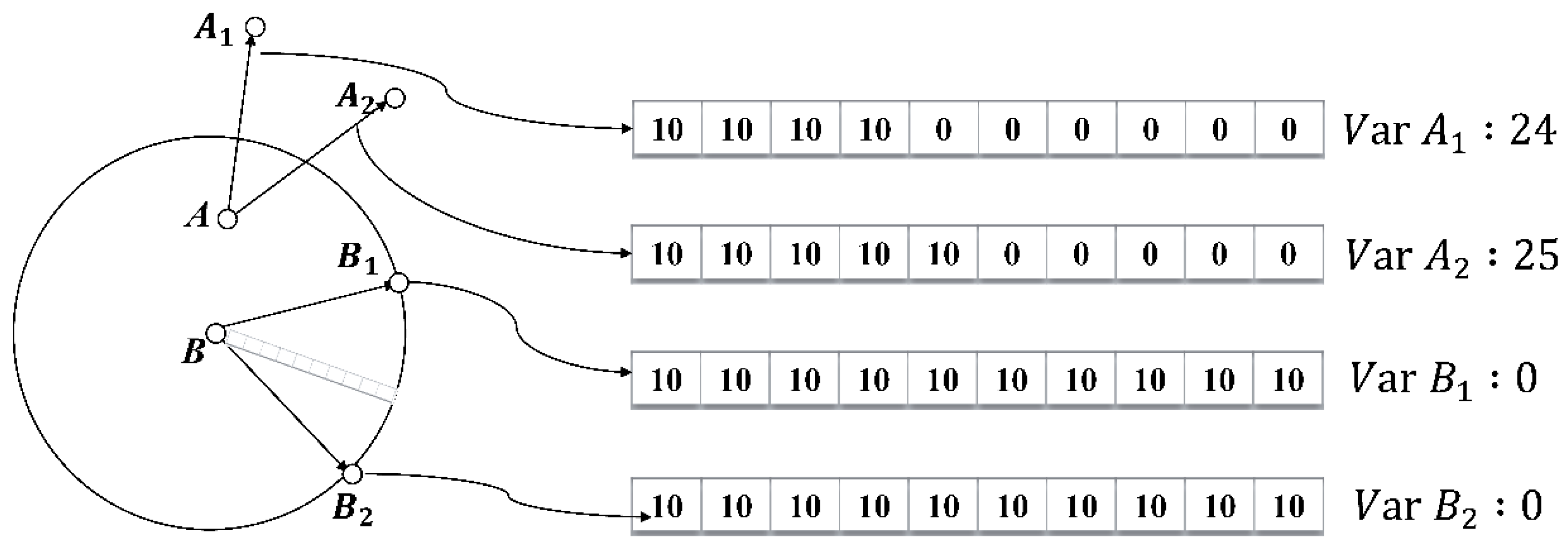
In this study, CNNs were designed to determine if an image with size of 34 × 34 was a center pivot irrigation system or not. Actually, the classifiers were used for detection of the center pivot systems. As described in the training data sampling approach, 25 images that were slightly off the center of a CPIS were selected as training data. Thus, more than one image of high possibility to be center pivot systems would be classified as center pivot systems using the classifier. To identify the center of each center pivot system with high accuracy, a variance based approach was used in the study.

This approach first calculates variance values of all pixels, and then the pixel with the lowest variance value within the local area is detected as the center point. Figure 8 provides an example to explain this approach.

Firstly, the true color image was converted to the gray image. A common formula in image processors, based on how human eyes perceive images, was used for the color conversion. The formula is described in Formula (1). Each pixel in the image had a gray value. Radius of the circle in Figure 8 goes through 10 pixels in the image. Point A locates within the circle. Point A₁ and A₂ are 10 pixels away from point A. The 10 pixels going through A and A₁ are considered as one pixel set. Variance values of the two pixel sets (from A to A₁, from A to A₂) are calculated and averaged. Averaged variance values of the two pixel sets were assigned to the variance value of A (24.5). Similarly, point B (center point) had a variance value of 0 with the same method. Color did not vary too much within the circle, whilst it changed rapidly on the edge of the circle. 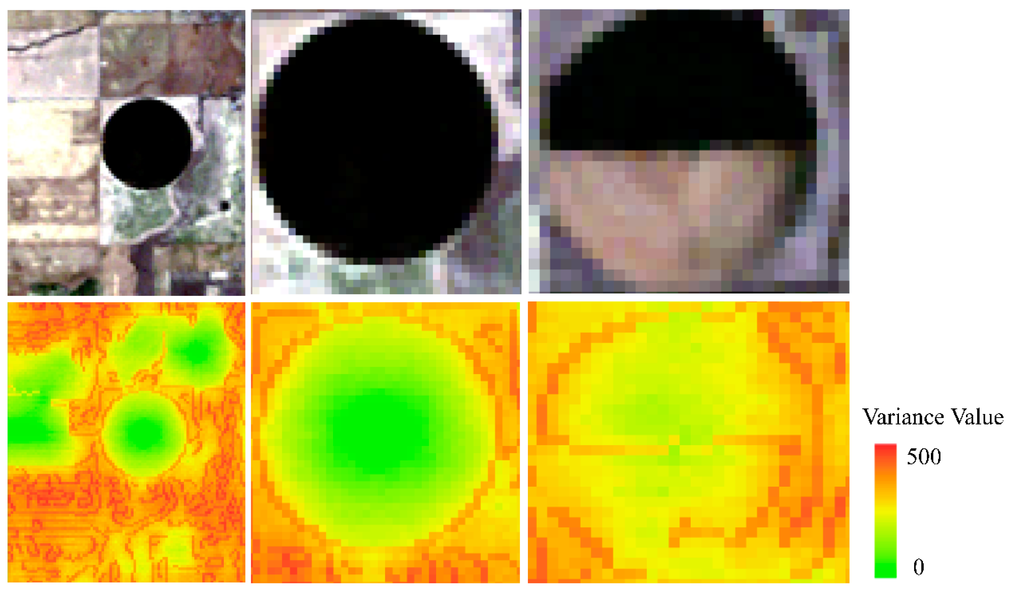As shown in Figure 9, images below the true color images were calculated using this approach.

Variance values of pixels were displayed by stretched colors from green to red. Green pixel indicates a low variance value, red pixel indicates a high variance value. Center points of the three center pivot systems were all displayed with green. Thus, the center point can be found by getting the lowest variance value among the nearest pixels, which are identified as center pivot systems by the classifier. In our experiments, 13 pixel sets toward different orientations were used for the calculation of the variance value for each pixel. Formula (2) was used for the variance calculation.

$$Gray=0.299\times Red+0.587\times Green+0.114\times Blue$$

(1)

$$s^2= \sum {\left(x-\overline{x}\right)}^2/N-1$$

(2)

5. Results

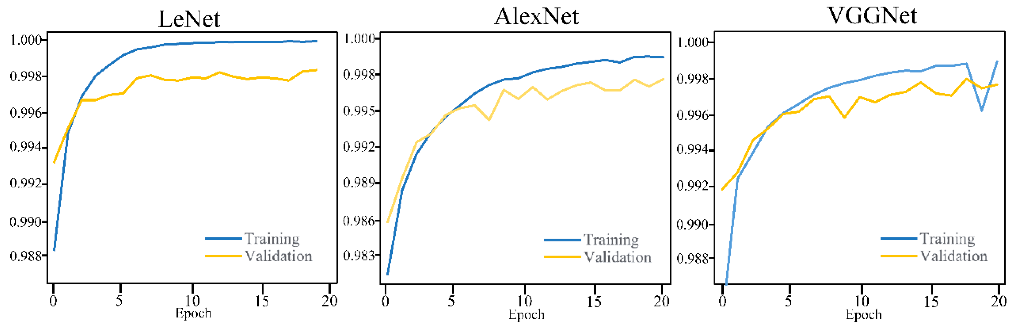
The work was implemented using the Keras API with TensorFlow as backend engines [46]. Training was performed on a machine with 24 cores and 100 GB of memory. Training the LeNet based network took about 9 h, the AlexNet based network more than 34 h due to a larger volume of parameters, and the VGGNet-based network was about 105 h due to its tremendous parameters. After training the three CNN models, their performances were compared and evaluated based on the training and validation sets. After iterating the training for 20 times, the Loss and Accuracy of each model is compared and presented in Figure 10 and Figure 11.

In Figure 10, the loss of all CNNs reached $e^{-2}$ level, which indicates that all models were well trained for the training and validation sets. The loss of the LeNet-based model dropped significantly and became a flat line after 6 epochs. AlexNet and VGGNet also dropped quickly to a satisfying level, within 20 epochs. Accuracies did not vary too much among the three CNNs. The LeNet-based network outperformed the other networks, with accuracy achieved being nearly 100% on the training set and 99.8% on the validation set. The AlexNet-based network achieved a high accuracy of 99.92% on the training set, and 99.76% on the validation set. Performing very close to the AlexNet-based network, the VGGNet-based network achieved 99.93% on the training set and 99.79% on the validation set.

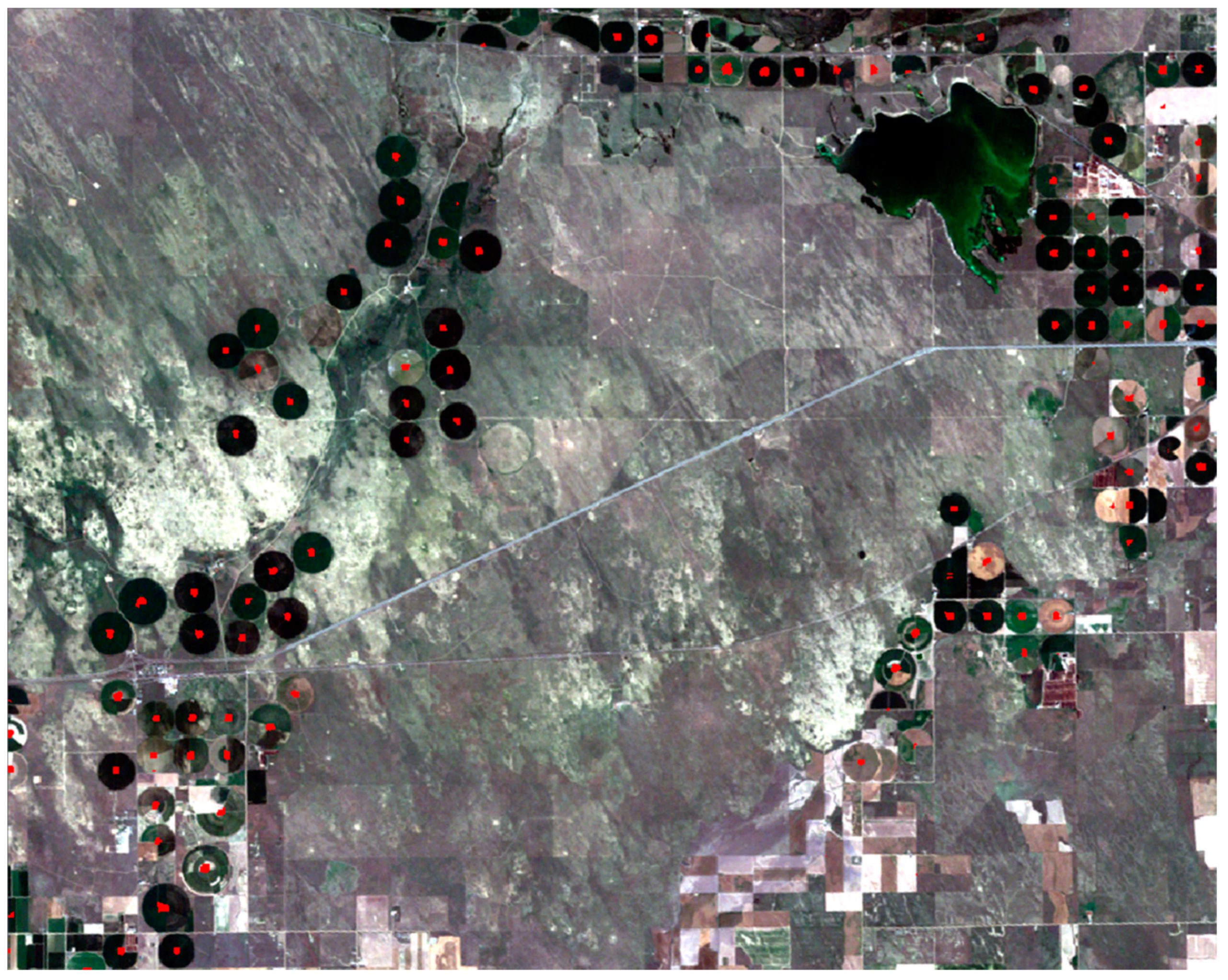
Due to its high performance and lower training time, the LeNet-based network was selected as the classifier for identifying the center pivot irrigation systems in the Landsat TM images. A test image with 4959 × 4744 × 3 pixels was fed to the classifier. By sliding a window with size of 34 × 34 over the test image, images with size of 34 × 34 × 3 were clipped and fed into the classifier. Output of the classifier was a probability for each class, where the class with highest probability compared to the other class was set as the class of the image. Part of the images processed after the classification are presented in Figure 12. The red-dot clusters represent areas that were identified as center pivot irrigation systems.

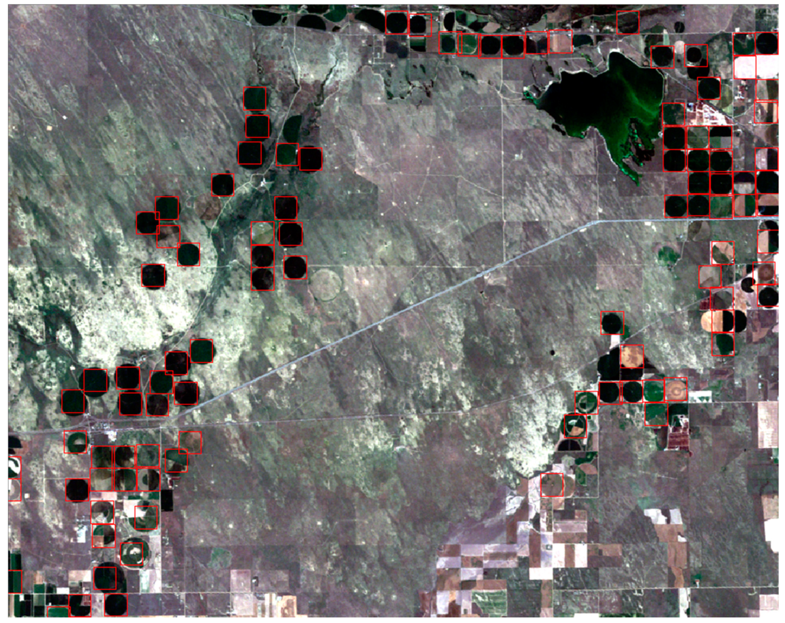
The more red-dots in a cluster, the more likely it is a center pivot. Different threshold values had been tested for screening out non-CPIS. The number 16 was found to have the best performance. Therefore, clusters that had less than 16 red dots were removed from the image for its low probability. The variance-based approach was then applied to the result of classification to locate the CPIS centers. Results are shown in Figure 13. It can be seen from Figure 13 that almost all center pivot irrigation systems were identified correctly.

To quantitatively analyze the classification results on the overall testing area, we manually identified all CPISs in the image. Precision and recall of the results were calculated and given in

Table 1. Quantity analysis results.

	Visually Observed CPISs	Identified CPISs	Correctly Identified CPISs
Count	1485	1446	1386

. Defined, precision tells us how many of the identified center pivots were correct, whilst recall tells us how many of the center pivots that should have been identified were actually identified. As shown in Table 1, there are 1485 CPISs that were visually observed in the testing area. Among them, 1446 were identified using the approach, and 1386 were correctly identified. The approach achieved a precision of 95.85% and a recall of 93.33%, which proved the high credibility of our approach.

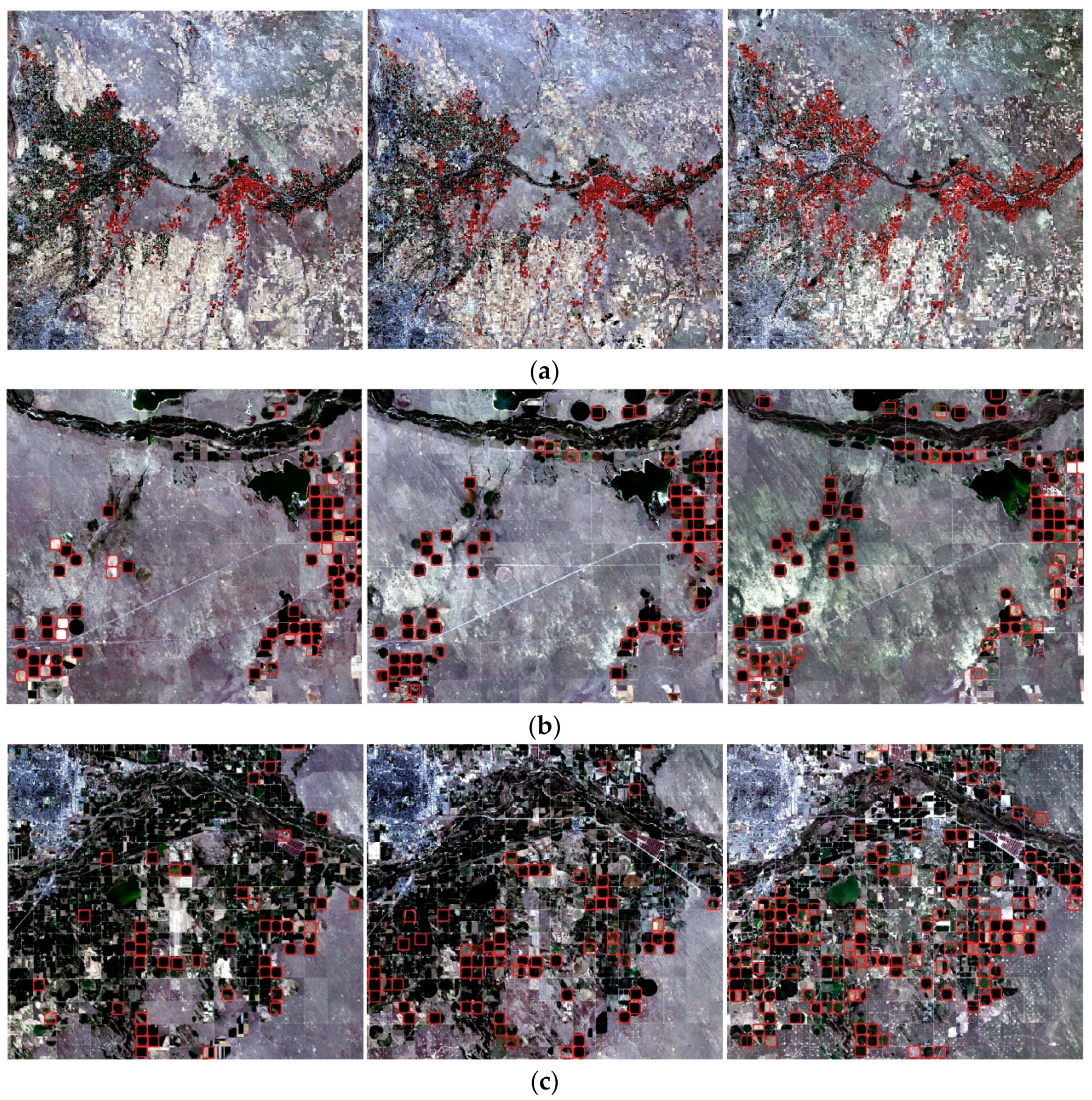
To further verify the availability using a pre-trained model for CPISs detection across different years, the classification model which was trained on data from 2011 was saved and experimented on images that collected in 1986 and 2000. Each image had 4959 × 4744 × 3 pixels and was fed into the same classifier. Structure and parameters of the classifier remained the same. Variance images were calculated, respectively, for each image. Since the national CDL data was not available until 2008, the non-irrigation fields were not filtered on images that were collected in 1986 and 2000. Results are shown in Figure 14.

Results of quantity analysis across different years is shown in

Table 2. Quantity analysis results in three different years.

Year	Count of Visually Observed CPISs	Count of Identified CPISs	Count of Correctly Identified CPISs
1986	960	807	782
2000	1179	956	941
2011	1485	1446	1386

. As shown in the table, for the year of 1986, a total of 960 CPISs were visually observed by human eyes. 807 CPISs were identified by the pre-trained model, which indicated a recall of 81%, where 782 out of 807 were correctly classified. Thus, a precision of 96% was achieved. For the image from 2000, 1179 CPISs were visually observed. The classifier identified 956 CPISs from the image. The count of the correctly identified CPISs was 941. Thus, a precision of 98% and a recall of 80% were achieved for the year 2000. The results of quantity analysis showed that both cases in 1986 and 2000, respectively, achieved a high classification precision and a satisfying recall using the classification model, which was pre-trained using data from 2011.

6. Discussion

This study had proposed a CNNs based approach for the identification of center pivot irrigation systems. Three modified CNNs based on different structures were constructed and compared. Training data collected in 2011 was fed into a CNN with the best performance, to train a classifier for CPISs detection. The pre-trained classifier was applied on images collected in two different years for validation. Here we discuss the strengths and weakness of our approach.

The proposed sampling approach was able to generate a large number of training images for training classifiers. Putting images that are slightly off the center of seed images into the training model can provide more help in extracting features. The fixed size of the window for image clipping was applied, considering most of the center pivot irrigation systems have a uniform size in the image. However, not all center pivot systems have the same size. A few of the center pivot systems that have much larger size failed to be identified using the model; however, the number of large center pivot irrigation systems was too small that it could be ignored. Though the large CPISs were ignored in this study, it can still be identified using this approach by training a classifier with a large CPIS training set.

As CNNs are a relatively black box model, the optimal combination of components needs to be determined empirically. We constructed and compared three representative CNNs with different layer combinations, for the task of CPIS identification. The network that consisted of two convolutional layers, two max pooling layers, and two fully connected layers performed better, and took relatively little time compared to the other networks for the same task. Deeper CNNs consisted of more convolutional layers, for example, AlexNet may also work on the low-resolution image recognition task, but its tremendous parameters may not help significantly for limited features extraction. A much more complicated network with more convolutional layers, the VGGNet-based network, performed very close to the AlexNet network on the low-resolution image classification task, but it took quite a long time on the training process compared to the simple CNN with higher performance. In this study, the training process was only iterated for 20 times for all models, for the purposes of comparison.

In this study, we used Landsat data acquired on 19 July 2011 to train a classifier. Images acquired on July 1985 and 2000, respectively, were fed into the pre-trained classifier to detect CPISs. Both cases achieved a high precision; however, the recalls of cases from 1985 and 2000 were lower than the case from 2011. That is because the classifier we used in the three cases was trained using data from 2011, and it was hard for the classifier to capture features that only existed in 1985 or 2000. Training a classifier based on images on the three years would have had a better performance in the three cases. Meanwhile, the color of CPIS on satellite images changes with seasons because of plant growing. CNNs extract features from both colors and shapes, so the CNNs trained in this study may not be suitable for classifying images from different seasons, which is a limitation of our model. This can be solved by training the model with training data covering different seasons. However, the bigger problem is to manually collect the training samples from lots of images, which is time and labor consuming. However, the model trained with all season data could potentially be used to identify CPISs from Landsat images, acquired in any season without re-training. The CNN used in this study was implemented on a machine without high-end graphic card supporting, which led to a long training time for each model.

7. Conclusions

The aim of this study was to automatically identify CPISs on Landsat images using CNNs. The proposed CNNs approach successfully identified CPISs with high accuracy. The variance based approach can effectively be used for locating the center of a CPIS identified by the classifier. This study also showed that the performance of deeper CNNs with complex structures is probably not better than that of simple CNNs with fewer layers, in low-resolution image classification and detection tasks. The credibility of our approach is supported by the high precision and recall of the results. Compared to the traditional method based on visual interpretation, the proposed automatic identification method provided a trustworthy solution for a wide range of rapid assessments of water and energy consumption, and can help in the long-term analysis of the impact of center pivot systems on landscapes and environments using remote sensing data. In future work, remote sensing images in different seasons will be collected and used to train models that can identify CPISs in Landsat images acquired in any season. The approach will also be incorporated into the geographical information service systems to assist in agriculture decision support.