Article

Geostatistical Determination of Soil Noise and Soil Phosphorus Spatial Variability

Institute of Agriculture and Environment, Massey University, Private Bag, Palmerston North 4474, New Zealand
*
Author to whom correspondence should be addressed.
Agriculture 2017, 7(10), 83; https://doi.org/10.3390/agriculture7100083
Submission received: 8 September 2017 / Revised: 25 September 2017 / Accepted: 27 September 2017 / Published: 28 September 2017

Abstract

:
This research studies the effect of stratifying soil samples to try and find a suitable depth to establish a geospatial relationship for a practical soil sampling grid in New Zealand hill country. Cores were collected from 200 predetermined sites in grids at two trial sites at “Patitapu” hill country farm in the Wairarapa, New Zealand. Trial 1 was a 200 m × 100 m grid located in a gently undulating paddock. Trial 2 was a 220 m × 80 m grid located on a moderately sloped paddock. Each grid had cores taken at intervals of 5 m, 10 m, or 20 m. Core sites were mapped out prior to going into the field; these points were found using a Leica Geo Systems GS15 (real time kinematic GPS) and marked with pigtail pegs and spray-paint on the ground. Cores were taken using a 50 mm-diameter soil core sampler. Cores were cut into three sections according to depth: A—0–30 mm, B—30–75 mm, and C—75–150 mm. Olsen P lab results were obtained for half of the total 1400 samples due to financial constraints. The results indicate that there was a significant decrease in variability from Section A to Section B for both trials. Section B and C for Trial 1 had similar variability, whereas there was another significant drop in variability from Section B to C in Trial 2. Measuring samples below the top 3 cm appeared to effectively reduce noise when sampled from 3 to 15 cm. However, measuring from 7.5 cm to 15 cm on the slope in Trial 2 reduced variability so much that all results were almost identical, which may mean that there is no measurable representation of plant available P. The reduction in noise by removing the top 3 cm of soil samples is significant for improving current soil nutrient testing methods by allowing better geospatial predictions for whole paddock soil nutrient variability mapping.

1. Introduction

Capital and or maintenance fertilizer applications are essential in sustaining New Zealand hill-country farms’ production and increasing their profit margin. Maintaining phosphorus (P) status is essential to encourage legume growth in pasture, and therefore nitrogen fixation. This is significant for optimizing pasture growth, especially in winter months [1]. The ideal Olsen P value ranges from 15–35 mg/kg on most sheep and beef properties; the value is dependent on soil type, amount of dry matter grown, rainfall, slope, and livestock enterprise variables [2]. The introduction of aerial applications of fertilizer since 1950 has allowed a significant increase in pasture production due to the reduction of nutrient limitations [3]. Superphosphate should be applied until sulphur (S) is not a limiting factor; S leaches as much as five times faster than P is lost by surface runoff and animal retention, and is much cheaper. In contrast, P should only be applied as one can afford [2]. However, the current practices of uniform farm management (e.g., blanket applications of fertilizer) are not efficient practices, and using aerial application technology is expensive [4]. If fertilizer is not applied efficiently, costs can exceed the benefits of application as excess nutrients end up in valleys and waterways, and other areas are either over- or under-fertilized [5]. It is necessary to more precisely determine the level of nutrients such as phosphate across a farm or paddock to inform fertilizer management decisions in order to variably apply fertilizer as required, which is now possible using computer-controlled technology [6].
If fertilizer application is to be improved, then a better understanding of the variability of soil nutrient levels both spatially and through the profile is required. Taking samples below the current 0–75 mm could reduce the impact of soil noise in the data (i.e., decrease variability) from animal excreta, which would improve the accuracy of current sampling methods, as data points with this noise are not representative of the surrounding area [7]. This research aims to determine the appropriate soil sampling depth to assess the spatial variability of soil Olsen P in order to produce a more accurate soil nutrient phosphorus map for variable rate fertilizer applications.

2. Materials and Methods
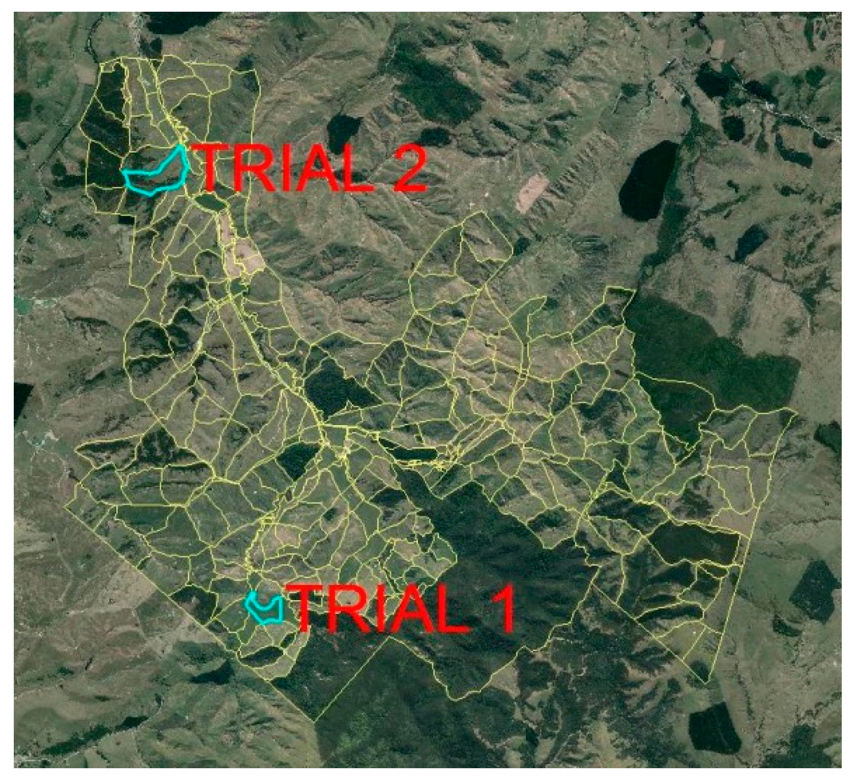
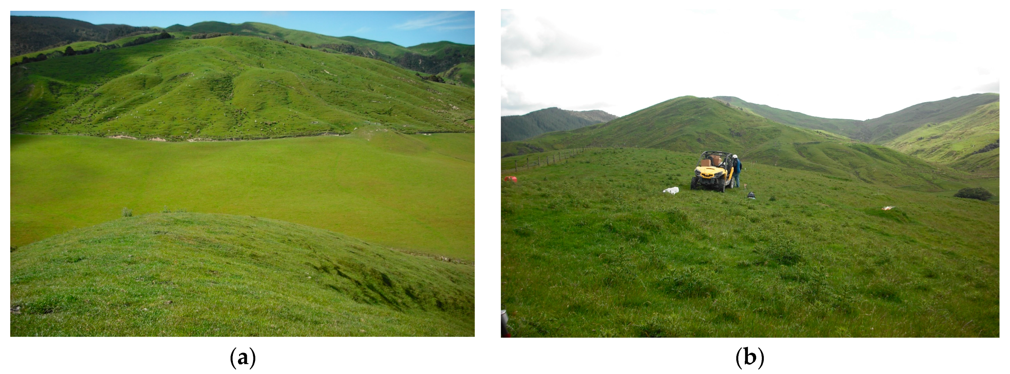
2.1. Site Selection

This research involved the collection of 200 samples from each of two trial sites: Trial 1 and Trial 2 (Figure 1), at “Patitapu” in the Wairarapa. The research site has annual applications of single superphosphate (0% N, 9% P, 0% K, 11% S, 20% Ca). The soil samples were collected the week before fertilizer was applied (i.e., one year after previous application). The sites were selected according to accessibility and slope. Trial 1 was located in a gently undulating paddock (Figure 2a). Sample cores were taken to a depth of greater than 15 cm. Trial 2 was located on a moderately-to-steeply-sloped paddock (Figure 2b). Cores were taken to a maximum depth of 15 cm due to difficulty in consistently coring deeper than this—especially on steeper, drier parts of the slope [8].

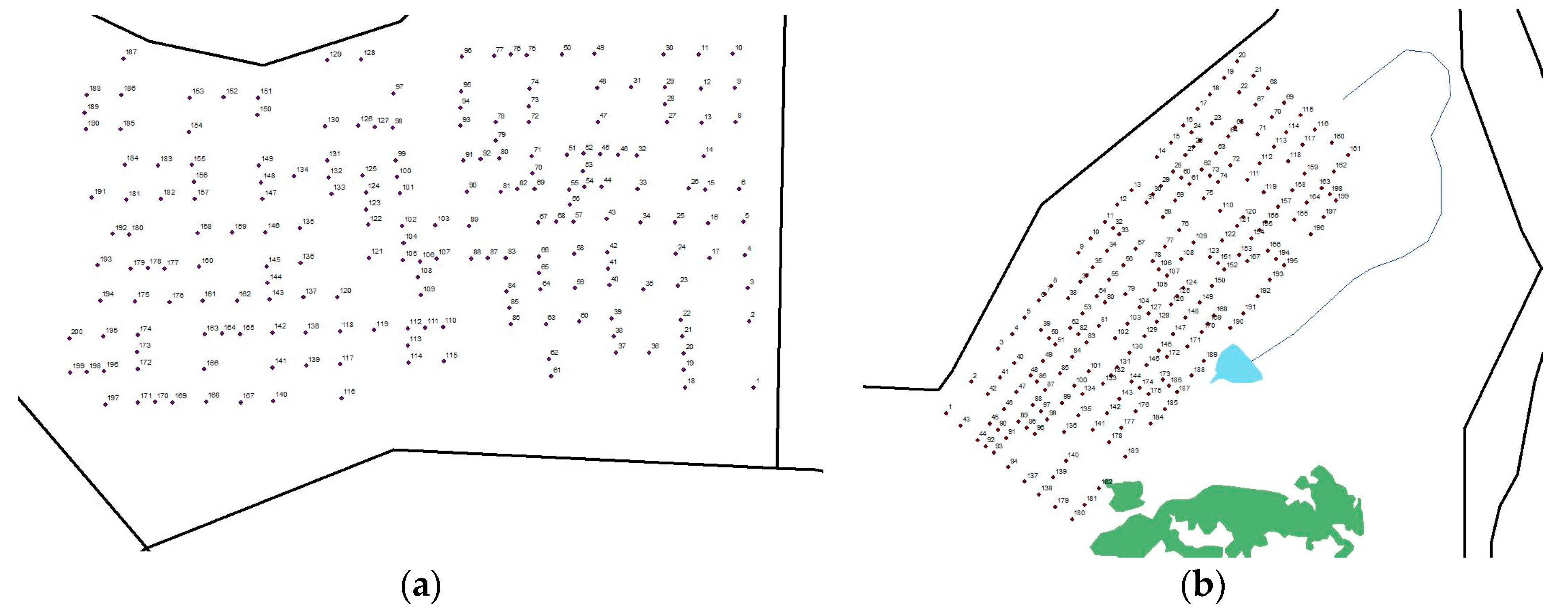
2.2. Core Collection Protocol

At each of the two trial sites, 200 cores were collected from a predetermined grid. Trial 1 was a 200 m × 100 m grid, and Trial 2 was a 220 m × 80 m grid. Grid size was determined by the shape and size of the paddocks for each site. Each grid had cores taken at intervals of 5 m, 10 m, and 20 m (Figure 3a,b). Core sites were mapped out on a Landsat 8 image (NASA) of the trial sites using ArcGIS 10.2 (ESRI, Redlands, CA, USA) prior to going into the field. This gave two sets of 200 GPS points that were then marked out using a Leica (real time kinematic GPS) to find the points, and pigtails and spray-paint on the ground to indicate where to take the core. Cores were taken using a 50 mm-diameter soil core sampler. Cores were laid in a plastic half pipe, wrapped in cling film “clingwrap”, put in a labelled re-sealable plastic bag, and placed inside a poster tube to prevent loss of moisture (Figure 4a–d). At the end of each day in the field, all cores were stored in a cooler until scanning. Each core site was photographed and scanned with the ASD (Analytic Spectral Devices, 1625 S. Fordham Street, Suite 300 Longmont, Colorado 80503, Boulder, CO, USA) to obtain hyperspectral data for the overlying vegetation. All core holes were filled with builders’ sand.

2.3. Sectioning of Soil Cores

Trial 1 cores were cut into four sections according to depth: A—0–30 mm, B—30–75 mm, C—75–150 mm, and D—>150 mm; and Trial 2 cores were cut into three sections: A—0–30 mm, B—30–75 mm, C—75–150 mm (Figure 5a,b). Each sample was ground using a pestle and mortar and sieved through a 2-mm sieve. Once dried and ground, each sample was scanned again using the ASD. Trial 1 Section D was not analysed for this research project due to the lack of a comparative Trial 2 Section D, as the subsoil on site 2 prevented sampling to layer D.

2.4. Measurement of Olsen P

Each air-dried sample was sieved through a 2-mm sieve and put into a labelled paper bag. One gram of each sample was weighed into a polycarbonate centrifuge tube. A 20 mL extract of sodium bicarbonate was added to each tube to remove any plant available phosphorus from the soil surface into the solution by replacing P with NaHCO3. These tubes were then placed into an end-over-end shaker for 30 min to allow time for the extraction to take place and separate the solid soil particles from the liquid extract containing the displaced phosphorus. Each tube was then immediately placed in a centrifuge for 3 min at 5000 rpm to further separate the fluids and solids. The extract was poured through 42 Whatman filter paper to remove any organic matter to complete the separation of solids and liquids. Once filtration was complete, a 4 mL aliquot of each sample was taken using a pipette and placed into 50 mL flasks. Approximately 10 mL of de-ionised water was added to each flask to dilute the solution in preparation for the addition of the strongly acidic reagent. Following this, the phosphomolybdate reagent solution was added and then extra de-ionised water was added to make up each flask to the 50 mL mark [9]. These were left for 20–30 min to allow the solutions to turn from yellow to blue. Once this reaction was complete, the blue colour was measured to infer Olsen P by filling a 1 cm cuvette with each sample and measuring absorbance at 712 nm using a spectrophotometer. The darker the blue was, the higher the absorbance, and thus the higher the Olsen P was. Each absorbance level was recorded and converted to Olsen P using Equation (1).
µg P/g soil = 40/0.420 × ¼ mL (aliquot of extract) × 20 mL (extract)/1 g (soil weight)
absorbance at 712 nm = 476.19 × absorbance (for 1 cm cuvette cell)

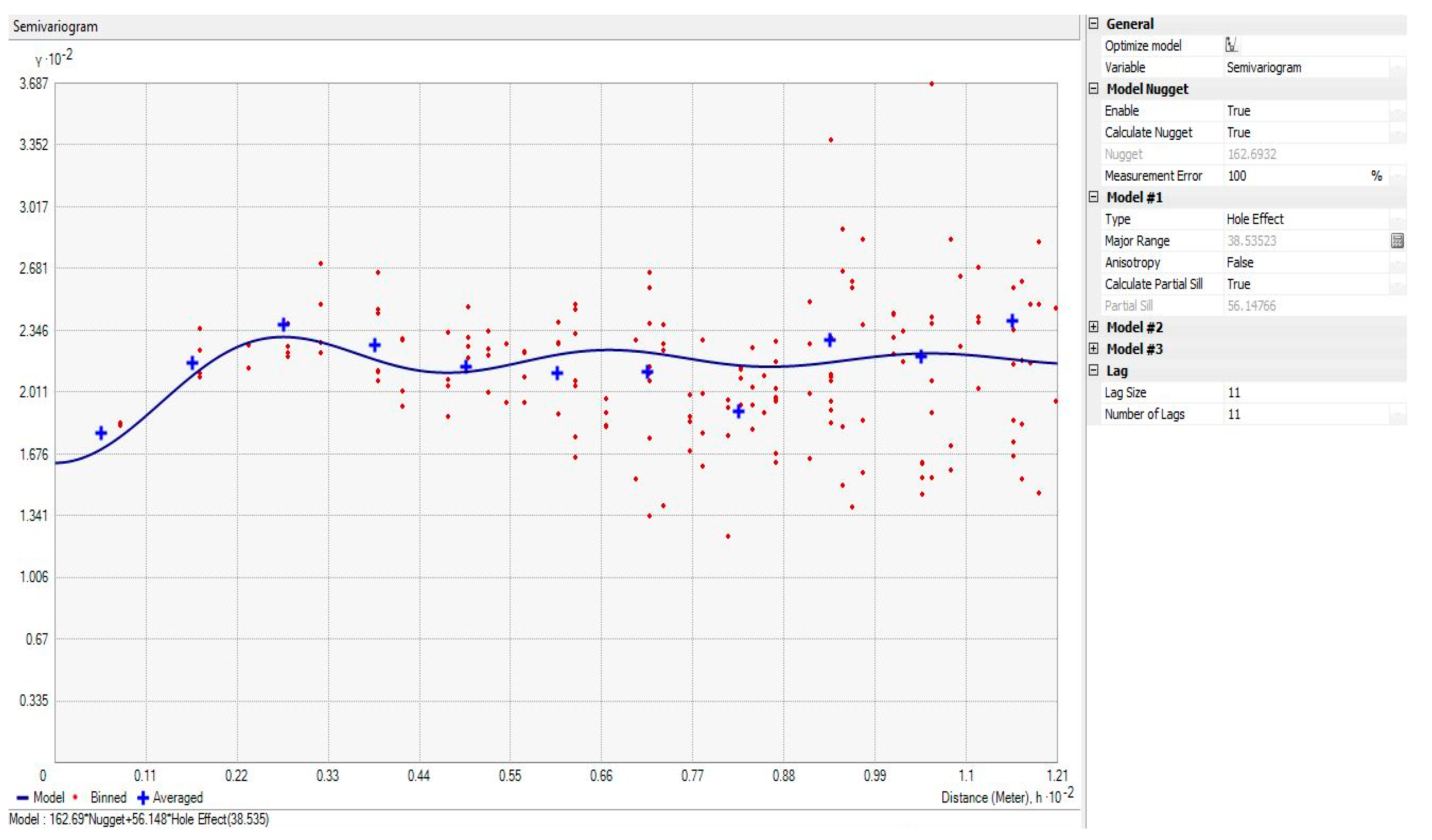
2.5. Geostatistical Analysis

Each level of each trial site was analysed according to the available data. Due to financial constraints, not all samples were tested for Olsen P. ArcGIS was used to create a variogram. Kriged prediction map and prediction error map for the A, B, and C sections of each trial site were performed. F-tests were completed to compare the variances of each data set within each trial and between each trial to determine which soil depths had the least variability.

3. Results

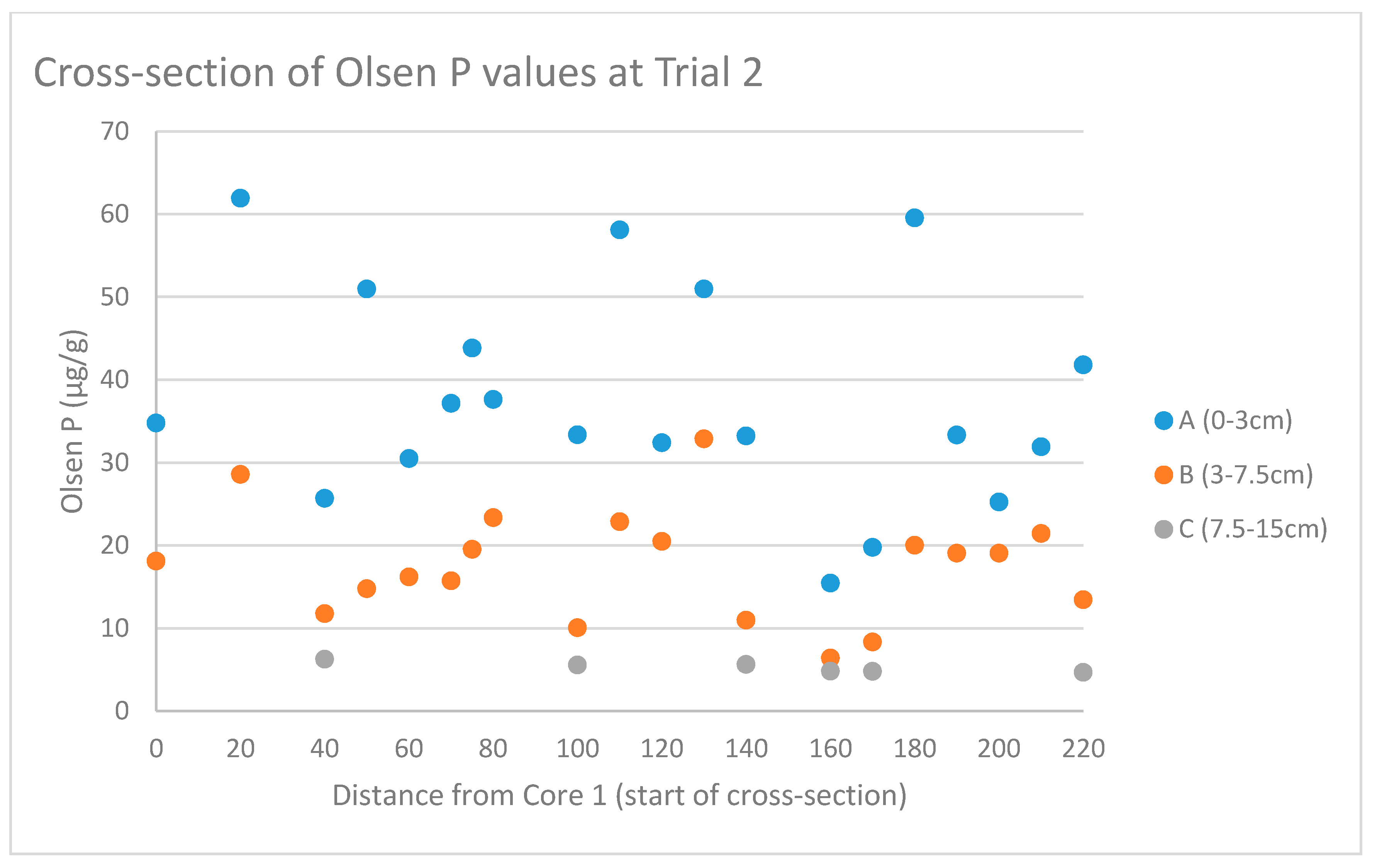
3.1. Spatial Variability of Phosphorus at Different Depth Ranges

Figure 6 shows a cross-section of Trial 2 from cores 1 to 20. This covers a distance of 220 m, with Olsen P values measured for Section A, B, and C at 5, 10, or 20 m intervals. It is evident that plant available phosphorus in soil varies significantly and seemingly randomly across the paddock along this transect for sections A and B. B is less variable than Section A, whilst Section C is fairly uniform; however, only six out of the possible 20 samples had measured Olsen P values along this transect due to the financial constraints that did not allow for measurement of Olsen P values for all Section C samples.
The two variograms seen below show an example of the best prediction model out of the six datasets (Figure 7) and one of the worst fitted prediction models (Figure 8) of all other variograms computed. The Trial 2 Section C variogram had the smallest nugget relative to the sill (Table 1) which is due to low variability, which increases spatial correlation, whereas the variogram for Trial 2 A had a large nugget relative to the sill (Table 1) which indicates too much noise in the data to give a good result for a Kriged prediction of Olsen P values, and hence not enough spatial correlation.

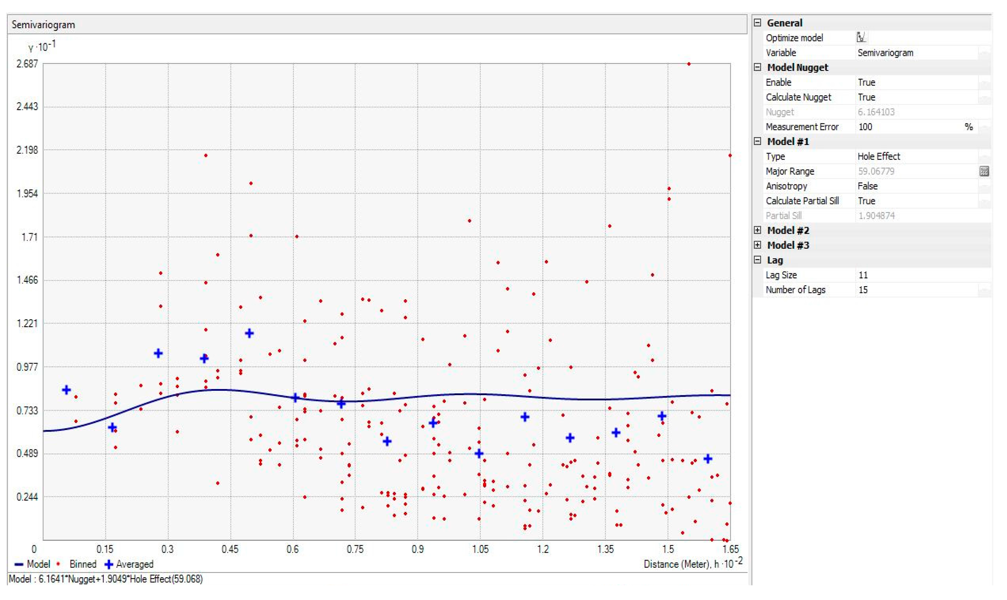
3.2. Variogram and Kriging Summary Statistics

Table 1 (Trial statistics for Trials 1 and 2) summarizes the statistical results of the variogram and Kriging analysis. The major range indicates the distance in metres, beyond which the data are no longer correlated. It would be expected to see the major range increasing downwards through the soil depth profile; however, this was not the case. Trial 1 Section A had a greater major range than the corresponding Sections B and C, the root mean square (RMS) and average standard error (ASE) were greater, which means that although the range was greater, the accuracy of prediction over this range was less and the data had a higher nugget value. The major range is calculated by the model equation, which is not an exact fit to the data and hence does not accurately portray the true major range of each dataset when there is a high RMS and or nugget value. The nugget, RMS, and ASE are better indicators to compare each dataset; in this case, the values decrease from A to C for both trials, which indicates an improved ability to Krige the data with depth. Overall, all datasets had a similar major range between 34 and 45 m, with the exception of Trial 2 Section C, which had a major range nearly double that of the other datasets at 59 m, likely due to the very low variability of this dataset.

3.3. Analysis of Variance (ANOVA)

A one-way F-test [10] was completed for this research report because two of the six datasets were significantly larger than the rest. The F-test shows which method of soil testing (i.e., which depth of soil measured) produced the least variability of Olsen P values, and whether the difference in population size of the A and B Trial 2 datasets had any significant effect on the data.

3.3.1. F-Test to Compare Trial Sites of Two Distinct Slope Classes

The F-test comparing the two trial sites—Trial 1 on a gently undulating site, and Trial 2 on a moderately steep site—showed that the overall variance of the two sites was unequal, and thus there was a statistically significant difference between the Olsen P values measured at each site. This suggests that either the topography or the difference in fertilizer application regimes of these different parts of Patitapu farm had an influence on the Olsen P values, and thus the two sites are independent in terms of measured Olsen P values. The results of the F-tests show that the A sections had equal variance, but the B and C sections had unequal variance. This means that although located on opposite ends of the Patitapu farm, the A sections did not have significantly different variances, suggesting that the Olsen P measurements for the top 3 cm could be equally “noisy” across the farm, irrespective of slope or location. The difference in B and C sections could suggest that at these depths the difference in slope and location significantly affects the Olsen P values.

3.3.2. F-test for Comparison of Variability of Sections within Each Trial

Where F < F-critical, there is no significant difference in the variance between the two methods with 95% confidence. The A sections compared to the B sections within each trial were significantly more variable for both trials, as were the A versus C. The variances of B and C sections were not significantly different for Trial 1, but for Trial 2 Section B had a higher variance than the corresponding Section C.

3.3.3. F-Test for Comparison of Variability of Different Sampling Methods

For both Trial 1 and Trial 2, there was no significant effect of removing the top 3 cm of soil and testing only from 3–7.5 cm on variability of Olsen P (Trial 1 F = 1.49, p > 0.05; and Trial 2 F = 1.26, p > 0.05) compared to sampling the top 7.5 cm. However, for both Trials, there was a significant reduction of variability when measuring from 3 to 15 cm compared to the standard 0–7.5 cm method (Trial 1 F = 1.65, p < 0.05; and Trial 2 F = 3.45, p < 0.05).

4. Discussion

The results of this research show that plant available phosphorus is highly variable and is difficult to Krige. The distances between cores taken for the two trial sites in this study were too great to allow for accurate Kriging. The current system of averaging samples taken across a transect may be the chosen method due to so much variability—making it hard to have a good method to accurately map the variability of phosphorus. However, according to literature and the results we have so far, there is definitely good potential for improving current soil sampling methods. This research shows that taking soil samples deeper in the soil profile (from 3 to 15 cm) will reduce the variability of the Olsen P values measured. This suggests that the top 3 cm includes a high level of statistical “noise” when included in current sampling depths (0–7.5 cm). However, measuring below 7.5 cm for a steeply sloped paddock such as Trial 2 may misrepresent the overall variability of soil P across a paddock or farm. This research project will help individual farmers and the wider industry by providing improved soil sampling methods, which should help farmers reach targeted levels of soil nutrients (Table 2).
Current soil testing methods in New Zealand for measuring the top 7.5 cm are derived from the early system of measuring to a 3 inch depth [2]. Current recommendations are still based on this research, which is why this measurement is still used. The present research shows that sampling to 15 cm and removing the top 3 cm before testing would provide a more stable soil test by eliminating soil noise, allowing for better geospatial representation. Although this may not be entirely representative of the depth over which plant roots obtain most of their nutrients, it makes it easier to map the relative variability of P across the farm.
The F-tests showed that the effect of noise in the top 3 cm of soil (Section A) was significant. The recommendation for soil sampling would be to measure from 3 to 15 cm to reduce statistical noise and improve the ability to Krige data. Overall the Kriges completed in this research proved that less variability of sample data allowed for more accurate Kriging. The major range for the data collected for this trial at distances no closer than 5 m apart varied across both trials and the A, B, and C sections from 34 to 59 m. This means that in future sampling could be completed at 30 m intervals and this should not worsen the standard errors of the Kriged predictions significantly at any of the three depth ranges up to 15 cm. There was no difference between the A sections (0–3 cm) of each trial, likely due to statistical noise disguising the base nutrient levels of the soil. The base nutrient levels of Section B in Trial 1 was higher than Section B of Trial 2; it is likely that the reduction of statistical noise allowed better detection of the base nutrient levels, which allowed for a distinction to be made between the two trial sites; i.e., between a gently undulating site and a moderately steep site.
Although the data collected for this thesis was insufficient to create Kriged prediction maps for Olsen P with a high level of accuracy (i.e., low prediction standard error), the intensity of data collected (60–200 samples over three depth ranges per site) relative to the 200 × 200 m and 220 × 80 m sites provides significantly more information than would be available in standard farm soil testing where there may be 60 samples for an entire 500-hectare farm. Thus, this research project has provided further valuable insight into the spatial variability of phosphorus in different slope classes on a typical hill country farm in New Zealand.
Hyperspectral data was collected for all soil samples used in this research project using an Analytical Spectral Device (ASD, Boulder, Co.). This can potentially be correlated with the Olsen P results to allow for the design of an algorithm that can predict Olsen P in situ. Additionally, hyperspectral data was collected for the pasture cover for each core site; this has potential for further analysis that will increase the understanding of how to use reflectance of pasture to determine the nutrient status of the underlying soil.

Acknowledgments

The Sports Turf Institute, Ravensdown Ltd., and The Institute of Agriculture and the Environment at Massey University provided financial support and the New Zealand Centre for Precision Agriculture provided staff support for field work.

Author Contributions

This work was conceived for a summer scholarship by Miles Grafton. The work was carried out by Therese Kaul. The analysis was undertaken by Therese Kaul with help from Miles Grafton. The results were obtained by Therese Kaul and the discussion was jointly undertaken by Therese Kaul and Miles Grafton.

Conflicts of Interest

The authors declare no conflict of interest. The sponsors had no role in the design of the study; in the collection, analyses, or interpretation of data; in the writing of the manuscript, and in the decision to publish the results.

References

  1. Morton, J.D.; Sinclair, A.G.; Morrison, J.D.; Smith, L.C.; Dodds, K.G. Balanced and adequate nutrition of phosphorus and sulphur in pasture. N. Z. Agric. Res. 1998, 41, 487–496. [Google Scholar] [CrossRef]
  2. Cornforth, I.S.; Sinclair, A.G. Fertiliser and Lime Recommendations for Pastures and Crops in New Zealand; Ministry of Agriculture and Fisheries: Wellington, New Zealand, 1984; 76p.
  3. Gillingham, A.G.; Morton, J.D.; Gray, A.H. Pasture responses to phosphorus and nitrogen fertilisers on East Coast hill country; total production from easy slopes. N. Z. Agric. Res. 2007, 50, 307–320. [Google Scholar] [CrossRef]
  4. Grafton, M.C.E.; Yule, I.J.; Lockhart, J.C. An Economic Analysis of the Topdressing Industry. In Farming’s Future: Minimizing Footprints and Maximizing Margins; Occasional Report No. 23; Currie, L.D., Christensen, C.L., Eds.; Fertilizer and Lime Research Centre, Massey University: Palmerston North, New Zealand, 2010; pp. 405–412. ISSN 0112-9902. [Google Scholar]
  5. Lucci, G.M.; McDowell, R.W.; Condron, L.M. Potential phosphorus and sediment loads from sources within a dairy farmed catchment. Soil Use Manag. 2010, 26, 44–52. [Google Scholar] [CrossRef]
  6. Chok, S.E.; Grafton, M.C.E.; Yule, I.J.; White, M. Accuracy of Differential Rate Application Technology for Aerial Spreading of Granular Fertilizer within New Zealand. In Proceedings of the 13th International Conference on Precision Agriculture, St. Louis, MO, USA, 31 July–3 August 2016. [Google Scholar]
  7. Morton, J.D.; Baird, D.B.; Manning, M.J. A soil sampling protocol to minimise the spatial variability in soil test values in New Zealand hill country. N. Z. Agric. Res. 2000, 43, 367–375. [Google Scholar] [CrossRef]
  8. Kaul, T.M.C.; Grafton, M.C.E.; Hedley, M.J.; Yule, I.J. Understanding soil phosphorus variability with depth for the improvement of current soil sampling methods. In Science and Policy: Nutrient Management Challenges for the Next Generation; Occasional Report No. 30; Fertilizer and Lime Research Centre, Massey University: Palmerston North, New Zealand, 2017; 11p, ISSN 0112-9902. [Google Scholar]
  9. Murphy, J.; Riley, J.P. A modified single solution method for the determination of phosphate in natural waters. Anal. Chim. Acta 1962, 27, 31–36. [Google Scholar] [CrossRef]
  10. Snedecor, G.W.; Cochran, W.G. Statistical Methods, 8th ed.; Iowa State University Press: Iowa City, IA, USA, 1989; ISBN 978-0-8138-1561-9. [Google Scholar]
Figure 1. Trial sites at Patitapu.
Agriculture 07 00083 g001
Figure 2. (a) Site 1; (b) Site 2.
Agriculture 07 00083 g002
Figure 3. (a) Site 1 grid pattern; (b) Site 2 grid pattern.
Agriculture 07 00083 g003
Figure 4. (a) Pigtail marker and core number; (b) Leica RTK GPS used to find grid sites; (c) Taking the 50 mm-diameter soil core; (d) Wrapping a core.
Agriculture 07 00083 g004
Figure 5. (a) A sectioned soil core (site 23 layer C), (b) Schematic of soil sections.
Agriculture 07 00083 g005
Figure 6. A cross-section of Trial 2 given as an example of phosphorus variability across the paddock where the trial is located.
Agriculture 07 00083 g006
Figure 7. Trial 2, Section C (7.5–15 cm) variogram best fit—this was the best prediction model out of all six, with a root mean square of 2.9 and a prediction error of 1.4 µg/g.
Agriculture 07 00083 g007
Figure 8. Trial 2, Section A variogram—this was one of the worst prediction models, with a root mean square of 14.6 and an average standard prediction error of 5.9 µg/g—this is likely due to the high variability of the measured Olsen P for this dataset.
Agriculture 07 00083 g008
Table 1. Summary of the variogram and Kriging statistics for both trials.
Trial 1
Root Mean SquareAverage Standard ErrorNuggetMajor RangePartial SillSillLag SizeNumber of LagsModel TypeNo. of Samples
aA10.46.6894549138911Hole Effect60
bB6.14.123432245810Hole Effect60
cC6.04.111433344710Hole Effect60
Trial 2
Root Mean SquareAverage Standard ErrorNuggetMajor RangePartial SillSillLag SizeNumber of LagsModel TypeNo. of Samples
aA14.65.916339562191111Hole Effect200
bB9.43.956342581811Hole Effect198
cC2.91.4659281115Hole Effect59
Table 2. These are the targeted levels of soil nutrients for each site according to slope [2].
Soil ParameterTrial 1 (Flat)Trial 2 (Steep)
Sulphur (S)30 mg/kg24 mg/kg
Potassium (K)20 mg/kg14 mg/kg
Phosphorus (P)25 mg/kg18 mg/kg

