
The Extraction of Torreya grandis Growing Areas Using a Spatial–Spectral Fused Attention Network and Multitemporal Sentinel-2 Images: A Case Study of the Kuaiji Mountain Region

Abstract
1. Introduction
2. Data and Methods
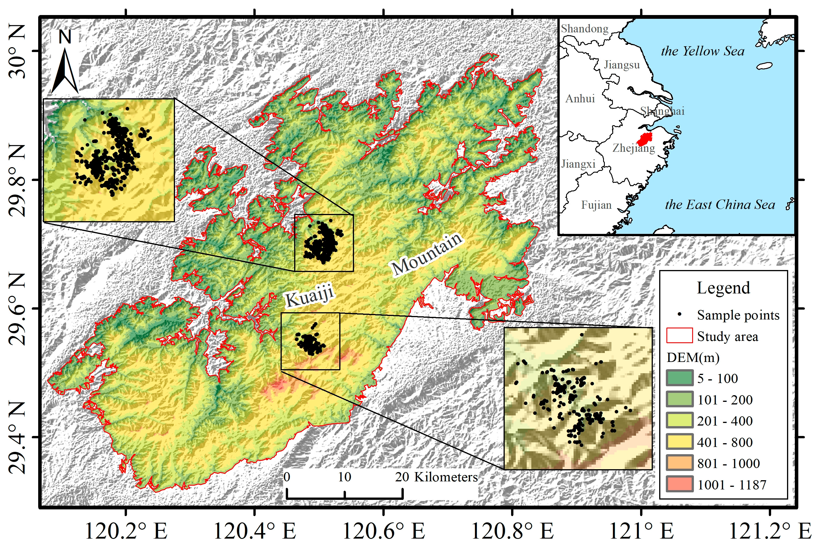
2.1. Study Area
2.2. Data
2.2.1. Sentinel-2 Data
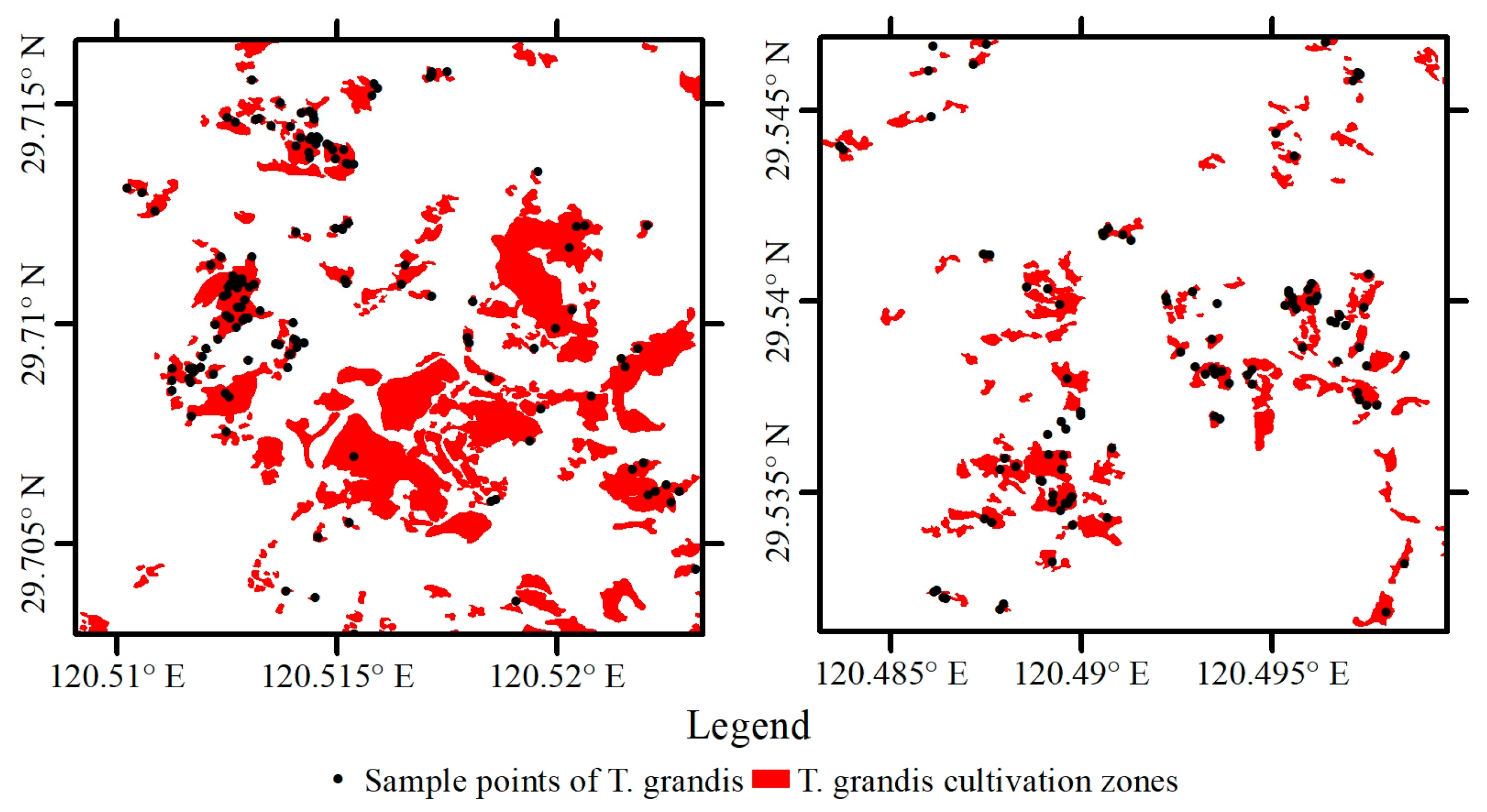
2.2.2. T. grandis Sample Data
2.2.3. Supplementary Data
2.3. Methods
2.3.1. Data Preprocessing
2.3.2. Feature Selection via the mRMR Algorithm
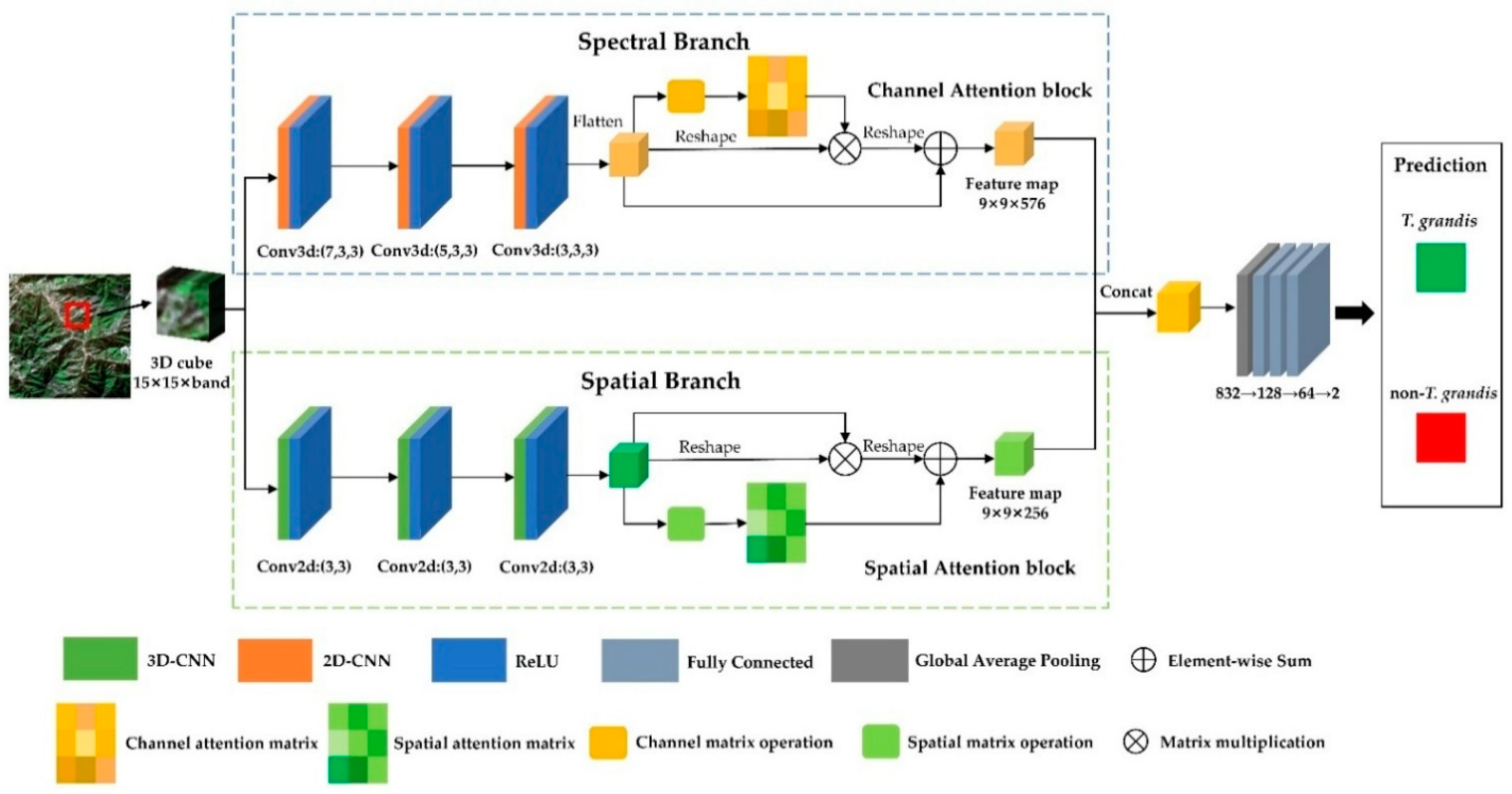
2.3.3. SSFAN
- 1.
- Spectral branch and spectral attention
- 2.
- Spatial branch and spatial attention
- 3.
- Feature fusion
2.3.4. Evaluation Methods
3. Result Analysis
3.1. Extraction of T. grandis Growing Areas Using the SSFAN
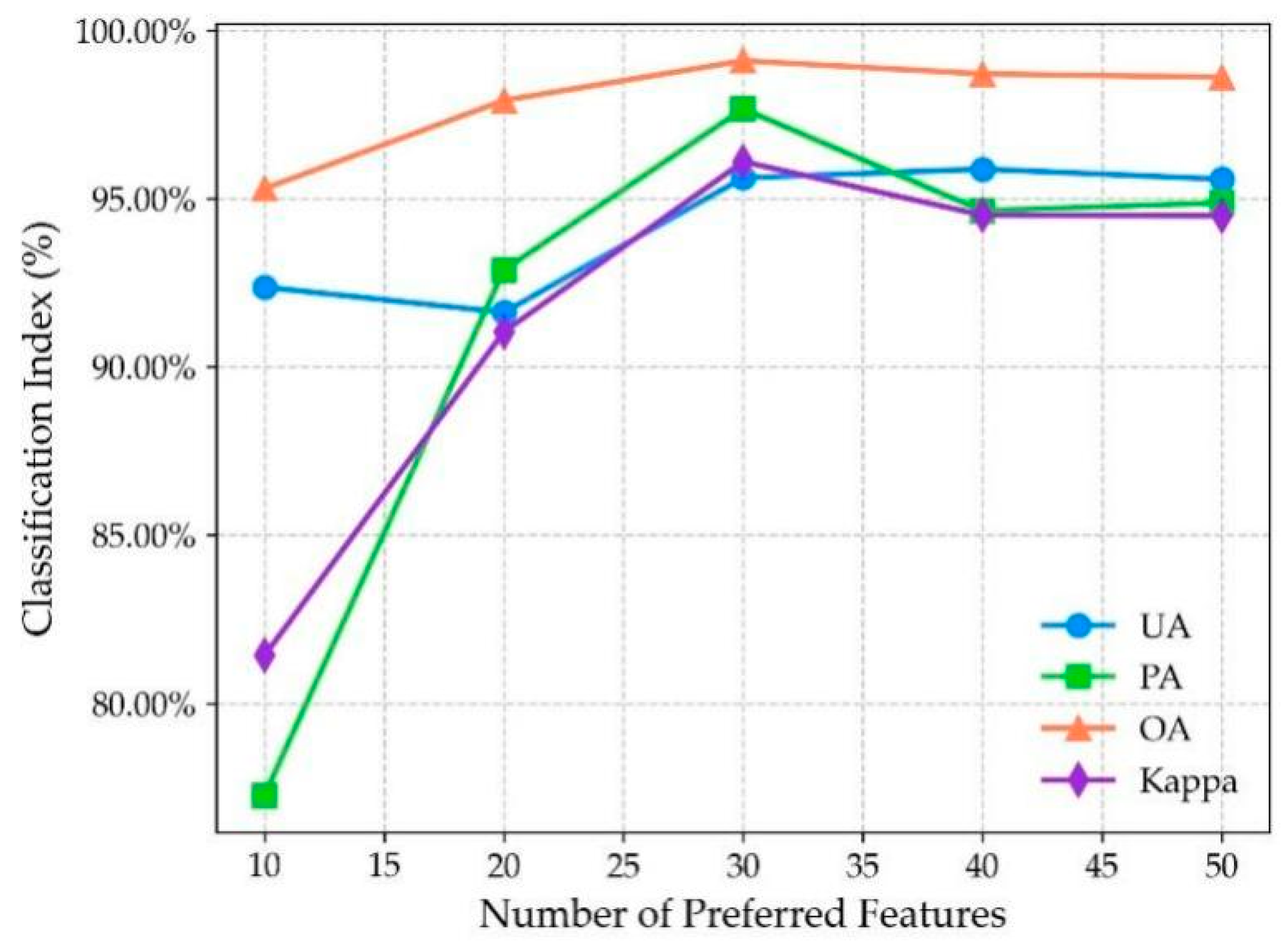
3.1.1. Feature Optimization
3.1.2. Deep Learning Environment Settings
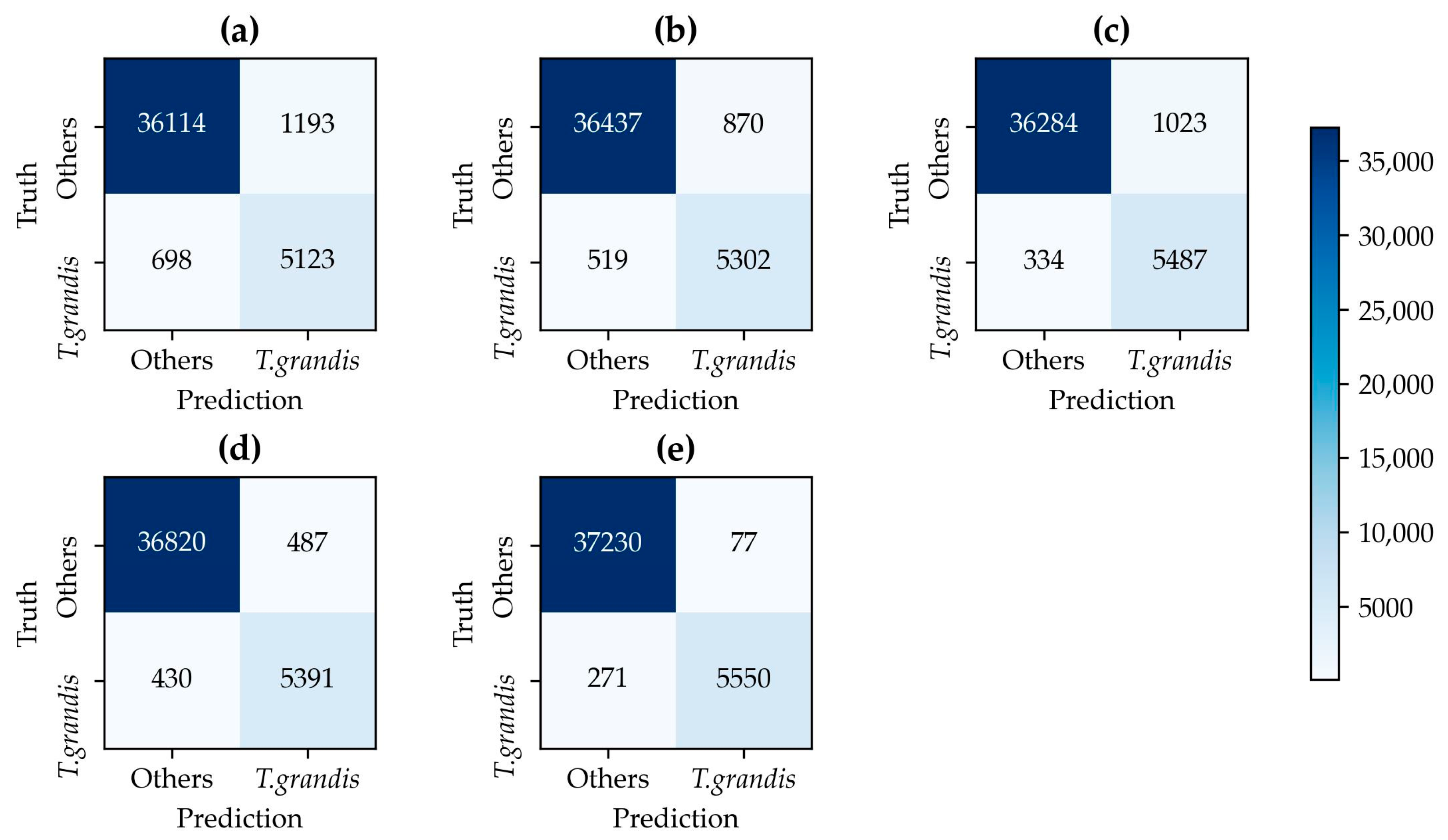
3.1.3. Model Validation and Extraction Results for T. grandis
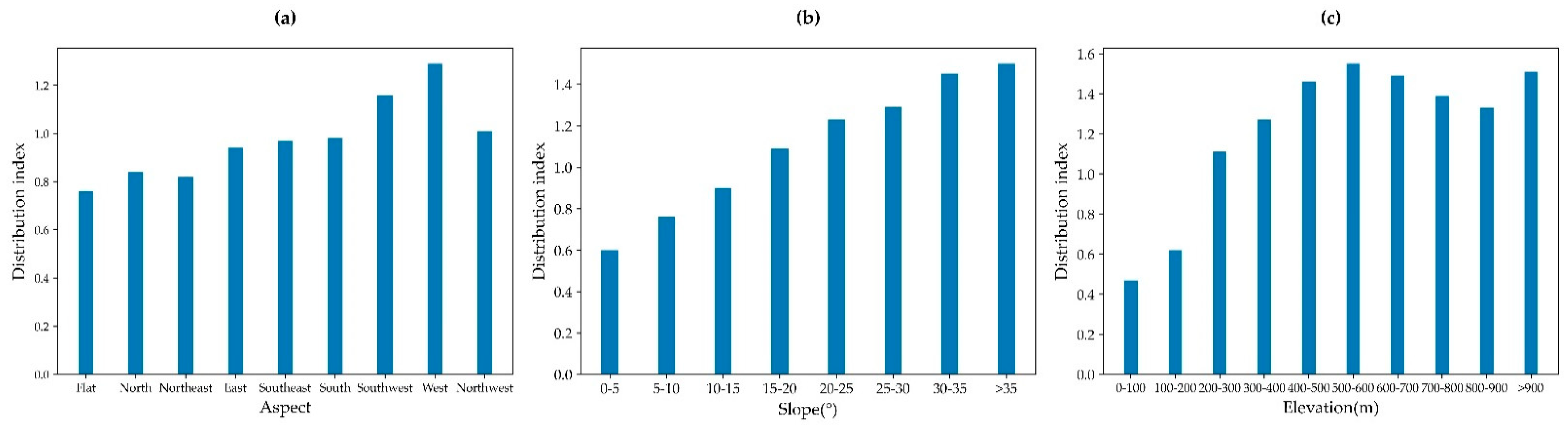
3.2. Analysis of the Distribution Characteristics of T. grandis
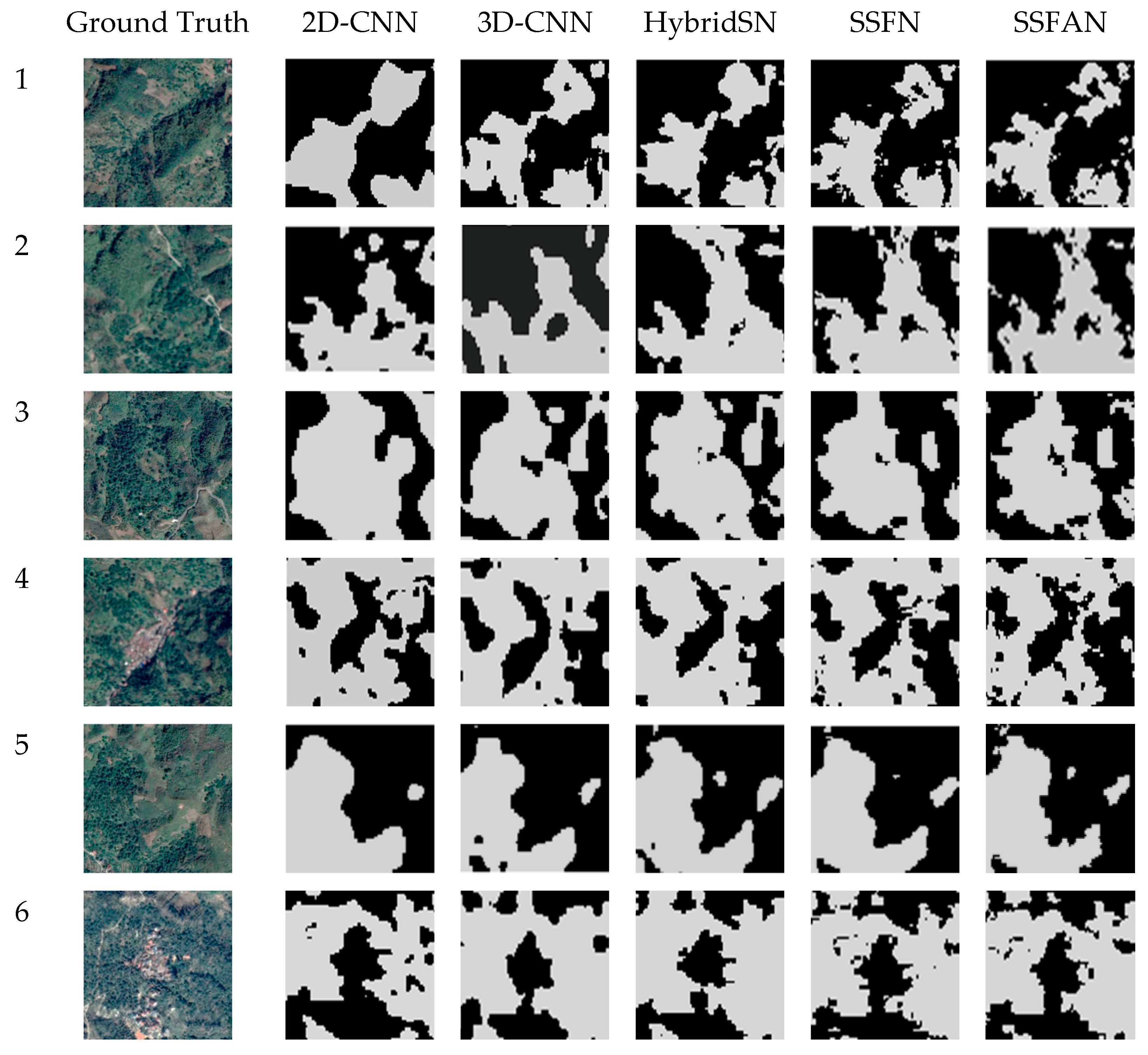
3.3. Comparison of Different Models
- 2D-CNN: Makantasis et al. described the specific network architecture [65]. This model is mainly based on the 2D-CNN.
- 3D-CNN: Zhang et al. described the specific network architecture [33]. This model is mainly based on the 3D-CNN.
- HybridSN: This hybrid model combines the 3D-CNN and 2D-CNN in a series. Roy et al. described the specific network architecture [66].
- SSFN: The attention mechanism is removed from the original SSFAN model, while the remainder of the structure remains unchanged.
4. Discussion
5. Conclusions
- On the basis of the spectral bands, vegetation indices, and texture features of 12 synthesized monthly average Sentinel-2 images from 2023, a hyperspectral image-like band structure was formed. After the mRMR feature selection, the SSFAN was constructed. The T. grandis growing areas in the Kuaiji Mountain area were extracted. The model’s accuracy was validated. The model achieved an OA of 99.1% and a Kappa coefficient of 0.961, with the UA and PA of T. grandis reaching 95.2% and 97.67%, respectively, indicating good extraction results.
- Elevation, aspect, and slope have significant impacts on the distribution of T. grandis. The distribution index of T. grandis is the most concentrated on the western, southern, and southwestern slopes, where light and heat conditions are more suitable. As slope steepness increased, the T. grandis distribution index exhibited an upward trend, with a particular preference for steep slopes (>20°). Additionally, regions at 500–600 m or greater elevation exhibited a relatively high distribution index.
- The test set was used to assess the evaluation indicators for each model. The performance ranking from highest to lowest was as follows: SSFAN > SSFN > HybridSN > 3D-CNN > 2D-CNN. The proposed model performed best and had an advantage in the extraction of T. grandis growing areas.
- In the extraction of T. grandis growing areas, the SSFAN, which fuses spectral and spatial features and introduces a self-attention mechanism, exhibited notable effectiveness and superiority. Additionally, the distribution of T. grandis is influenced by a combination of natural and human factors, providing a valuable scientific basis for the planting and management of T. grandis.
Author Contributions
Funding
Institutional Review Board Statement
Data Availability Statement
Acknowledgments
Conflicts of Interest
References
- Milad, M.; Schaich, H.; Bürgi, M.; Konold, W. Climate change and nature conservation in Central European forests: A review of consequences, concepts and challenges. For. Ecol. Manag. 2011, 261, 829–843. [Google Scholar] [CrossRef]
- Nunes, L.J.R.; Meireles, C.I.R.; Gomes, C.J.P.; Ribeiro, N.M.C.A. The Impact of Climate Change on Forest Development: A Sustainable Approach to Management Models Applied to Mediterranean-Type Climate Regions. Plants 2021, 11, 69. [Google Scholar] [CrossRef] [PubMed]
- Chen, X.; Jin, H. A Case Study of Enhancing Sustainable Intensification of Chinese Torreya Forest in Zhuji of China. Environ. Nat. Resour. Res. 2019, 9, 53–60. [Google Scholar] [CrossRef]
- Chen, X.; Jin, H. Review of cultivation and development of Chinese torreya in China. For. Trees Livelihoods 2018, 28, 68–78. [Google Scholar] [CrossRef]
- Cook, B.I.; Mankin, J.S.; Anchukaitis, K.J. Climate Change and Drought: From Past to Future. Curr. Clim. Chang. Rep. 2018, 4, 164–179. [Google Scholar] [CrossRef]
- Ramos, M.C.; Martínez-Casasnovas, J.A. Climate change influence on runoff and soil losses in a rainfed basin with Mediterranean climate. Nat. Hazards 2015, 78, 1065–1089. [Google Scholar] [CrossRef]
- Skendzic, S.; Zovko, M.; Zivkovic, I.P.; Lesic, V.; Lemic, D. The Impact of Climate Change on Agricultural Insect Pests. Insects 2021, 12, 440. [Google Scholar] [CrossRef]
- Han, N.; Zhang, X.; Wang, X.; Wang, K. Extraction of Torreya grandis Merrillii based on object-oriented method from IKONOS imagery. J. Zhejiang Univ. (Agric. Life Sci.) 2009, 35, 670–676. [Google Scholar] [CrossRef]
- Han, N.; Zhang, X.; Wang, X.; Chen, L.; Wang, K. Identification of distributional information Torreya Grandis Merrlllii using high resolution imagery. J. Zhejiang Univ. (Eng. Sci.) 2010, 44, 420–425. [Google Scholar]
- Wang, Y. Distribution Information Extraction and Dynamic Change Monitoring of Torreya Grandis Based on Multi-Source Data. Master’s Thesis, Zhejiang A&F University, Hangzhou, China, 2017. [Google Scholar]
- Ji, J.; Yu, X.; Yu, C.; Zhang, Y.; Li, D. The Spatial Distribution Extraction of Torreya grandis Forest Based on Remote Sensing and Random Forest. South China Agric. 2018, 12, 93–95. [Google Scholar] [CrossRef]
- Axelsson, A.; Lindberg, E.; Reese, H.; Olsson, H. Tree species classification using Sentinel-2 imagery and Bayesian inference. Int. J. Appl. Earth Obs. Geoinf. 2021, 100, 102318. [Google Scholar] [CrossRef]
- Franklin, S.E.; Ahmed, O.S. Deciduous tree species classification using object-based analysis and machine learning with unmanned aerial vehicle multispectral data. Int. J. Remote Sens. 2017, 39, 5236–5245. [Google Scholar] [CrossRef]
- Bjerreskov, K.S.; Nord-Larsen, T.; Fensholt, R. Forest type and tree species classification of nemoral forests with Sentinel-1 and 2 Time Series data. Preprints 2021. [Google Scholar] [CrossRef]
- Ghorbanian, A.; Zaghian, S.; Asiyabi, R.M.; Amani, M.; Mohammadzadeh, A.; Jamali, S. Mangrove Ecosystem Mapping Using Sentinel-1 and Sentinel-2 Satellite Images and Random Forest Algorithm in Google Earth Engine. Remote Sens. 2021, 13, 2565. [Google Scholar] [CrossRef]
- Guo, Q.; Zhang, J.; Guo, S.; Ye, Z.; Deng, H.; Hou, X.; Zhang, H. Urban Tree Classification Based on Object-Oriented Approach and Random Forest Algorithm Using Unmanned Aerial Vehicle (UAV) Multispectral Imagery. Remote Sens. 2022, 14, 3885. [Google Scholar] [CrossRef]
- Modzelewska, A.; Fassnacht, F.E.; Sterenczak, K. Tree species identification within an extensive forest area with diverse management regimes using airborne hyperspectral data. Int. J. Appl. Earth Obs. Geoinf. 2020, 84, 101960. [Google Scholar] [CrossRef]
- Nasiri, V.; Beloiu, M.; Darvishsefat, A.A.; Griess, V.C.; Maftei, C.; Waser, L.T. Mapping tree species composition in a Caspian temperate mixed forest based on spectral-temporal metrics and machine learning. Int. J. Appl. Earth Obs. Geoinf. 2023, 116, 103154. [Google Scholar] [CrossRef]
- Nguyen, H.M.; Demir, B.; Dalponte, M. Weighted support vector machines for tree species classification using lidar data. In Proceedings of the IGARSS 2019-2019 IEEE International Geoscience and Remote Sensing Symposium, Yokohama, Japan, 28 July–2 August 2019; pp. 6740–6743. [Google Scholar]
- Yang, G.; Zhao, Y.; Li, B.; Ma, Y.; Li, R.; Jing, J.; Dian, Y. Tree Species Classification by Employing Multiple Features Acquired from Integrated Sensors. J. Sens. 2019, 2019, 3247946. [Google Scholar] [CrossRef]
- Alzubaidi, L.; Zhang, J.; Humaidi, A.J.; Al-Dujaili, A.; Duan, Y.; Al-Shamma, O.; Santamaría, J.; Fadhel, M.A.; Al-Amidie, M.; Farhan, L. Review of deep learning: Concepts, CNN architectures, challenges, applications, future directions. J. Big Data 2021, 8, 53. [Google Scholar] [CrossRef]
- La Rosa, L.E.C.; Sothe, C.; Feitosa, R.Q.; de Almeida, C.M.; Schimalski, M.B.; Oliveira, D.A.B. Multi-task fully convolutional network for tree species mapping in dense forests using small training hyperspectral data. ISPRS J. Photogramm. Remote Sens. 2021, 179, 35–49. [Google Scholar] [CrossRef]
- Li, Q.; Wong, F.K.K.; Fung, T. Mapping multi-layered mangroves from multispectral, hyperspectral, and LiDAR data. Remote Sens. Environ. 2021, 258, 112403. [Google Scholar] [CrossRef]
- Zhao, H.; Zhong, Y.; Wang, X.; Hu, X.; Luo, C.; Boitt, M.; Piiroinen, R.; Zhang, L.; Heiskanen, J.; Pellikka, P. Mapping the distribution of invasive tree species using deep one-class classification in the tropical montane landscape of Kenya. ISPRS J. Photogramm. Remote Sens. 2022, 187, 328–344. [Google Scholar] [CrossRef]
- Wei, X.; Yu, X.; Liu, B.; Zhi, L. Convolutional neural networks and local binary patterns for hyperspectral image classification. Eur. J. Remote Sens. 2019, 52, 448–462. [Google Scholar] [CrossRef]
- Xi, Y.; Ren, C.; Wang, Z.; Wei, S.; Bai, J.; Zhang, B.; Xiang, H.; Chen, L. Mapping Tree Species Composition Using OHS-1 Hyperspectral Data and Deep Learning Algorithms in Changbai Mountains, Northeast China. Forests 2019, 10, 818. [Google Scholar] [CrossRef]
- Fricker, G.A.; Ventura, J.D.; Wolf, J.A.; North, M.P.; Davis, F.W.; Franklin, J. A Convolutional Neural Network Classifier Identifies Tree Species in Mixed-Conifer Forest from Hyperspectral Imagery. Remote Sens. 2019, 11, 2326. [Google Scholar] [CrossRef]
- Sothe, C.; De Almeida, C.M.; Schimalski, M.B.; La Rosa, L.E.C.; Castro, J.D.B.; Feitosa, R.Q.; Dalponte, M.; Lima, C.L.; Liesenberg, V.; Miyoshi, G.T.; et al. Comparative performance of convolutional neural network, weighted and conventional support vector machine and random forest for classifying tree species using hyperspectral and photogrammetric data. GIScience Remote Sens. 2020, 57, 369–394. [Google Scholar] [CrossRef]
- Guan, H.; Yu, Y.; Yan, W.; Li, D.; Li, J. 3D-Cnn Based Tree species classification using mobile lidar data. Int. Arch. Photogramm. Remote Sens. Spat. Inf. Sci. 2019, 42, 989–993. [Google Scholar] [CrossRef]
- Liu, M.H.; Han, Z.W.; Chen, Y.M.; Liu, Z.; Han, Y.S. Tree species classification of LiDAR data based on 3D deep learning. Measurement 2021, 177, 109301. [Google Scholar] [CrossRef]
- Mäyrä, J.; Keski-Saari, S.; Kivinen, S.; Tanhuanpää, T.; Hurskainen, P.; Kullberg, P.; Poikolainen, L.; Viinikka, A.; Tuominen, S.; Kumpula, T.; et al. Tree species classification from airborne hyperspectral and LiDAR data using 3D convolutional neural networks. Remote Sens. Environ. 2021, 256, 112322. [Google Scholar] [CrossRef]
- Nezami, S.; Khoramshahi, E.; Nevalainen, O.; Pölönen, I.; Honkavaara, E. Tree species classification of drone hyperspectral and RGB imagery with deep learning convolutional neural networks. Remote Sens. 2020, 12, 1070. [Google Scholar] [CrossRef]
- Zhang, B.; Zhao, L.; Zhang, X. Three-dimensional convolutional neural network model for tree species classification using airborne hyperspectral images. Remote Sens. Environ. 2020, 247, 111938. [Google Scholar] [CrossRef]
- Liang, J.; Li, P.; Zhao, H.; Han, L.; Qu, M. Forest species classification of UAV hyperspectral image using deep learning. In Proceedings of the 2020 Chinese Automation Congress (CAC), Shanghai, China, 6–8 November 2020; pp. 7126–7130. [Google Scholar]
- Shi, C.; Liao, D.; Xiong, Y.; Zhang, T.; Wang, L. Hyperspectral Image Classification Based on Dual-Branch Spectral Multiscale Attention Network. IEEE J. Sel. Top. Appl. Earth Obs. Remote Sens. 2021, 14, 10450–10467. [Google Scholar] [CrossRef]
- Xu, J.; Li, K.; Li, Z.; Chong, Q.; Xing, H.; Xing, Q.; Ni, M. Fuzzy graph convolutional network for hyperspectral image classification. Eng. Appl. Artif. Intell. 2024, 127, 107280. [Google Scholar] [CrossRef]
- Hou, C.; Liu, Z.; Chen, Y.; Wang, S.; Liu, A. Tree Species Classification from Airborne Hyperspectral Images Using Spatial–Spectral Network. Remote Sens. 2023, 15, 5679. [Google Scholar] [CrossRef]
- Fu, J.; Liu, J.; Tian, H.; Li, Y.; Bao, Y.; Fang, Z.; Lu, H. Dual attention network for scene segmentation. In Proceedings of the IEEE/CVF Conference on Computer Vision and Pattern Recognition, Long Beach, CA, USA, 15–20 June 2019; pp. 3146–3154. [Google Scholar]
- Li, R.; Zheng, S.; Duan, C.; Yang, Y.; Wang, X. Classification of Hyperspectral Image Based on Double-Branch Dual-Attention Mechanism Network. Remote Sens. 2020, 12, 582. [Google Scholar] [CrossRef]
- Mura, M.; Bottalico, F.; Giannetti, F.; Bertani, R.; Giannini, R.; Mancini, M.; Orlandini, S.; Travaglini, D.; Chirici, G. Exploiting the capabilities of the Sentinel-2 multi spectral instrument for predicting growing stock volume in forest ecosystems. Int. J. Appl. Earth Obs. Geoinf. 2018, 66, 126–134. [Google Scholar] [CrossRef]
- Ferreira, M.P.; Wagner, F.H.; Aragao, L.; Shimabukuro, Y.E.; de Souza, C.R. Tree species classification in tropical forests using visible to shortwave infrared WorldView-3 images and texture analysis. Isprs J. Photogramm. Remote Sens. 2019, 149, 119–131. [Google Scholar] [CrossRef]
- Liu, L.X.; Coops, N.C.; Aven, N.W.; Pang, Y. Mapping urban tree species using integrated airborne hyperspectral and LiDAR remote sensing data. Remote Sens. Environ. 2017, 200, 170–182. [Google Scholar] [CrossRef]
- Valderrama-Landeros, L.; Flores-de-Santiago, F.; Kovacs, J.M.; Flores-Verdugo, F. An assessment of commonly employed satellite-based remote sensors for mapping mangrove species in Mexico using an NDVI-based classification scheme. Environ. Monit. Assess. 2017, 190, 23. [Google Scholar] [CrossRef]
- Persson, M.; Lindberg, E.; Reese, H. Tree species classification with multi-temporal Sentinel-2 data. Remote Sens. 2018, 10, 1794. [Google Scholar] [CrossRef]
- Sefrin, O.; Riese, F.M.; Keller, S. Deep Learning for Land Cover Change Detection. Remote Sens. 2020, 13, 78. [Google Scholar] [CrossRef]
- Russo, L.; Mauro, F.; Memar, B.; Sebastianelli, A.; Gamba, P.; Ullo, S.L. Using Multi-Temporal Sentinel-1 and Sentinel-2 data for water bodies mapping. arXiv 2024, arXiv:2402.00023. [Google Scholar] [CrossRef]
- Sukmono, A.; Hadi, F.; Widayanti, E.; Nugraha, A.L.; Bashit, N. Identifying Burnt Areas in Forests and Land Fire Using Multitemporal Normalized Burn Ratio (NBR) Index on Sentinel-2 Satellite Imagery. Int. J. Saf. Secur. Eng. 2023, 13, 469–477. [Google Scholar] [CrossRef]
- Tavus, B.; Kocaman, S.; Gokceoglu, C. Flood damage assessment with Sentinel-1 and Sentinel-2 data after Sardoba dam break with GLCM features and Random Forest method. Sci. Total Environ. 2022, 816, 151585. [Google Scholar] [CrossRef]
- Louis, J.; Debaecker, V.; Pflug, B.; Main-Knorn, M.; Bieniarz, J.; Mueller-Wilm, U.; Cadau, E.; Gascon, F. Sentinel-2 Sen2Cor: L2A processor for users. In Proceedings of the Living Planet Symposium 2016, Prague, Czech Republic, 9–13 May 2016; pp. 1–8. [Google Scholar]
- Sentinel Application Platform (SNAP). Available online: https://step.esa.int/main/toolboxes/snap/ (accessed on 20 December 2024).
- Zheng, H.; Du, P.; Chen, J.; Xia, J.; Li, E.; Xu, Z.; Li, X.; Yokoya, N. Performance evaluation of downscaling Sentinel-2 imagery for land use and land cover classification by spectral-spatial features. Remote Sens. 2017, 9, 1274. [Google Scholar] [CrossRef]
- Qi, H.; Tian, W.; Zhang, X. Index System of Landform Regionalization for Highway in China. J. Chang. Univ. Nat. Sci. Ed. 2011, 31, 33–38. [Google Scholar]
- Rouse Jr, J.W.; Haas, R.H.; Deering, D.; Schell, J.; Harlan, J.C. Monitoring the Vernal Advancement and Retrogradation (Green Wave Effect) of Natural Vegetation; NASA: Washington, DC, USA, 1974. [Google Scholar]
- Gitelson, A.A.; Kaufman, Y.J.; Merzlyak, M.N. Use of a green channel in remote sensing of global vegetation from EOS-MODIS. Remote Sens. Environ. 1996, 58, 289–298. [Google Scholar] [CrossRef]
- Huete, A.R. A soil-adjusted vegetation index (SAVI). Remote Sens. Environ. 1988, 25, 295–309. [Google Scholar] [CrossRef]
- Huete, A.; Didan, K.; Miura, T.; Rodriguez, E.P.; Gao, X.; Ferreira, L.G. Overview of the radiometric and biophysical performance of the MODIS vegetation indices. Remote Sens. Environ. 2002, 83, 195–213. [Google Scholar] [CrossRef]
- Frampton, W.J.; Dash, J.; Watmough, G.; Milton, E.J. Evaluating the capabilities of Sentinel-2 for quantitative estimation of biophysical variables in vegetation. ISPRS J. Photogramm. Remote Sens. 2013, 82, 83–92. [Google Scholar] [CrossRef]
- Fitzgerald, G.; Rodriguez, D.; Christensen, L.; Belford, R.; Sadras, V.; Clarke, T. Spectral and thermal sensing for nitrogen and water status in rainfed and irrigated wheat environments. Precis. Agric. 2006, 7, 233–248. [Google Scholar] [CrossRef]
- Jiang, K.; Zhao, Q.; Wang, X.; Sheng, Y.; Tian, W. Tree Species Classification for Shelterbelt Forest Based on Multi-Source Remote Sensing Data Fusion from Unmanned Aerial Vehicles. Forests 2024, 15, 2200. [Google Scholar] [CrossRef]
- Tassi, A.; Vizzari, M. Object-Oriented LULC Classification in Google Earth Engine Combining SNIC, GLCM, and Machine Learning Algorithms. Remote Sens. 2020, 12, 3776. [Google Scholar] [CrossRef]
- Yang, S.; Gu, L.; Li, X.; Jiang, T.; Ren, R. Crop Classification Method Based on Optimal Feature Selection and Hybrid CNN-RF Networks for Multi-Temporal Remote Sensing Imagery. Remote Sens. 2020, 12, 3119. [Google Scholar] [CrossRef]
- Liu, G.; Jiang, X.; Tang, B. Application of feature optimization and convolutional neural network in crop classification. J. Geoinf. Sci. 2021, 23, 1071–1081. [Google Scholar]
- Peng, H.; Long, F.; Ding, C. Feature selection based on mutual information: Criteria of max-dependency, max-relevance, and min-redundancy. IEEE Trans. Pattern Anal. Mach. Intell. 2005, 27, 1226–1238. [Google Scholar] [CrossRef]
- Sun, L.; Chen, H.; Pan, J. Analysis of the land use spatiotemporal variation based on DEM—Beijing Yanqing County as an example. J. Mt. Res. 2004, 22, 762–766. [Google Scholar]
- Makantasis, K.; Karantzalos, K.; Doulamis, A.; Doulamis, N. Deep supervised learning for hyperspectral data classification through convolutional neural networks. In Proceedings of the 2015 IEEE International Geoscience and Remote Sensing Symposium (IGARSS), Milan, Italy, 26–31 July 2015; pp. 4959–4962. [Google Scholar]
- Roy, S.K.; Krishna, G.; Dubey, S.R.; Chaudhuri, B.B. HybridSN: Exploring 3D–2D CNN Feature Hierarchy for Hyperspectral Image Classification. IEEE Geosci. Remote Sens. Lett. 2020, 17, 277–281. [Google Scholar] [CrossRef]
- Zhong, Z.; Wang, J.; Wen, Y.; Zhang, Q. Research on the Resource Development and Industrialization Strategies of Chinese Torreya grandis. J. Zhejiang Agric. Sci. 2023, 64, 3020–3025. [Google Scholar]
- Wu, L.; Yang, L.; Li, Y.; Shi, J.; Zhu, X.; Zeng, Y. Evaluation of the Habitat Suitability for Zhuji Torreya Based on Machine Learning Algorithms. Agriculture 2024, 14, 1077. [Google Scholar] [CrossRef]
- Yang, X.; Yao, H.; Fan, F.; Yan, F.; Li, K.; Chen, C.; Wu, L. Effects of different altitudes on Torreya grandis ‘Merrillii’ fruit quality and its comprehensive evaluation. J. Anhui Agric. Univ. 2023, 50, 792–797. [Google Scholar] [CrossRef]


| Band Name | Central Wavelength (μm) | Spatial Resolution (m) |
|---|---|---|
| B1—Coastal aerosol | 0.443 | 60 |
| B2—Blue | 0.490 | 10 |
| B3—Green | 0.560 | 10 |
| B4—Red | 0.665 | 10 |
| B5—Vegetation Red Edge 1 | 0.705 | 20 |
| B6—Vegetation Red Edge 2 | 0.740 | 20 |
| B7—Vegetation Red Edge 3 | 0.783 | 20 |
| B8—NIR | 0.842 | 10 |
| B8A—Vegetation Red Edge 4 | 0.865 | 20 |
| B9—Water vapor | 0.945 | 60 |
| B10—SWIR Cirrus | 1.375 | 60 |
| B11—SWIR | 1.610 | 20 |
| B12—SWIR | 2.190 | 20 |
| Name | Calculation Formulas |
|---|---|
| NDVI [53] | |
| GNDVI [54] | |
| SAVI [55] | |
| EVI [56] | |
| S2REP [57] | |
| NDREI [58] |
| Rank | Category | Name | Rank | Category | Name |
|---|---|---|---|---|---|
| 1 | Vegetation index (May) | GNDVI | 16 | Spectral feature (Mar) | B4 |
| 2 | Texture feature (Apr) | CORR | 17 | Spectral feature (May) | B11 |
| 3 | Vegetation index (Nov) | S2REP | 18 | Spectral feature (May) | B3 |
| 4 | Spectral feature (May) | B5 | 19 | Vegetation index (Mar) | EVI |
| 5 | Vegetation index (Mar) | GNDVI | 20 | Vegetation index (Nov) | NDREI |
| 6 | Spectral feature (Jul) | B9 | 21 | Spectral feature (Apr) | B11 |
| 7 | Vegetation index (Dec) | S2REP | 22 | Spectral feature (Mar) | B3 |
| 8 | Vegetation index (May) | S2REP | 23 | Spectral feature (May) | B12 |
| 9 | Vegetation index (Jul) | GNDVI | 24 | Vegetation index (Jan) | GNDVI |
| 10 | Vegetation index (Apr) | NDVI | 25 | Spectral feature (Mar) | B2 |
| 11 | Spectral feature (Jul) | B12 | 26 | Spectral feature (Mar) | B12 |
| 12 | Vegetation index (Feb) | GNDVI | 27 | Spectral feature (Apr) | B5 |
| 13 | Texture feature (Nov) | CORR | 28 | Texture feature (Mar) | CORR |
| 14 | Texture feature (Jun) | ENT | 29 | Vegetation index (Oct) | S2REP |
| 15 | Spectral feature (Jul) | B11 | 30 | Spectral feature (May) | B4 |
| Patch Size | Initial Learning Rate | Batch Size | Epoch | Loss Function |
|---|---|---|---|---|
| 15 | 0.01 | 64 | 200 | cross entropy loss |
| Method | Data Set | Class | UA (%) | PA (%) | OA (%) | Kappa |
|---|---|---|---|---|---|---|
| 2D-CNN | Train | T. grandis non-T. grandis | 94.56 99.60 | 98.32 98.66 | 98.40 | 0.955 |
| Validation | T. grandis non-T. grandis s | 91.10 96.97 | 82.45 98.59 | 96.18 | 0.843 | |
| Test | T. grandis non-T. grandis | 81.11 98.10 | 88.14 96.80 | 95.62 | 0.818 | |
| 3D-CNN | Train | T. grandis non-T. grandis | 97.16 99.72 | 99.09 99.72 | 99.11 | 0.975 |
| Validation | T. grandis non-T. grandis | 91.22 97.83 | 88.12 98.52 | 96.92 | 0.867 | |
| Test | T. grandis non-T. grandis | 91.08 97.67 | 85.90 98.60 | 96.78 | 0.865 | |
| HybridSN | Train | T. grandis non-T. grandis | 99.16 99.82 | 99.42 99.74 | 99.66 | 0.990 |
| Validation | T. grandis non-T. grandis | 93.68 97.36 | 84.71 99.01 | 96.87 | 0.872 | |
| Test | T. grandis non-T. grandis | 94.26 97.26 | 84.29 99.09 | 96.85 | 0.871 | |
| SSFN | Train | T. grandis non-T. grandis | 98.51 99.70 | 99.04 99.54 | 99.42 | 0.983 |
| Validation | T. grandis non-T. grandis | 92.21 98.89 | 92.50 98.85 | 97.92 | 0.911 | |
| Test | T. grandis non-T. grandis | 92.61 98.69 | 91.71 98.85 | 97.87 | 0.909 | |
| SSFAN | Train | T. grandis non-T. grandis | 98.61 99.73 | 99.12 99.57 | 99.46 | 0.985 |
| Validation | T. grandis non-T. grandis | 94.85 99.81 | 98.71 99.20 | 99.14 | 0.962 | |
| Test | T. grandis non-T. grandis | 95.62 99.64 | 97.67 99.32 | 99.11 | 0.961 |
Disclaimer/Publisher’s Note: The statements, opinions and data contained in all publications are solely those of the individual author(s) and contributor(s) and not of MDPI and/or the editor(s). MDPI and/or the editor(s) disclaim responsibility for any injury to people or property resulting from any ideas, methods, instructions or products referred to in the content. |
© 2025 by the authors. Licensee MDPI, Basel, Switzerland. This article is an open access article distributed under the terms and conditions of the Creative Commons Attribution (CC BY) license (https://creativecommons.org/licenses/by/4.0/).
Share and Cite
Lyu, Y.; Wang, Y.; Shen, X. The Extraction of Torreya grandis Growing Areas Using a Spatial–Spectral Fused Attention Network and Multitemporal Sentinel-2 Images: A Case Study of the Kuaiji Mountain Region. Agriculture 2025, 15, 829. https://doi.org/10.3390/agriculture15080829
Lyu Y, Wang Y, Shen X. The Extraction of Torreya grandis Growing Areas Using a Spatial–Spectral Fused Attention Network and Multitemporal Sentinel-2 Images: A Case Study of the Kuaiji Mountain Region. Agriculture. 2025; 15(8):829. https://doi.org/10.3390/agriculture15080829
Chicago/Turabian StyleLyu, Yanyan, Yong Wang, and Xiaoling Shen. 2025. "The Extraction of Torreya grandis Growing Areas Using a Spatial–Spectral Fused Attention Network and Multitemporal Sentinel-2 Images: A Case Study of the Kuaiji Mountain Region" Agriculture 15, no. 8: 829. https://doi.org/10.3390/agriculture15080829
APA StyleLyu, Y., Wang, Y., & Shen, X. (2025). The Extraction of Torreya grandis Growing Areas Using a Spatial–Spectral Fused Attention Network and Multitemporal Sentinel-2 Images: A Case Study of the Kuaiji Mountain Region. Agriculture, 15(8), 829. https://doi.org/10.3390/agriculture15080829