2.1. Method for Calculating Virtual Water for Food Imports
Virtual water content measurement research is mainly carried out from the following two perspectives. On the one hand, classification is based on virtual water content. There are two main methods. One approach is grounded in the water footprint theory, which assesses the volume of water resources needed for the cultivation of individual agricultural products, thereby providing an estimate of the virtual water trade associated with those products [
27]. The other is a method based on input–output data to estimate the amount of virtual water trade in different industries, sectors, and products [
5,
28]. On the other hand, it is classified according to the perspective of the object and region involved. From the perspective of the object involved, it is mainly focused on the measurement of virtual water in different agricultural products. The measurement of the virtual water content of agricultural products mainly considers climatic factors, soil conditions, crop types, and growth cycles [
26,
29]. Furthermore, when analyzing the driving forces of virtual water flows, most studies use methods such as gravity models, factor decomposition, and commonality analysis [
30,
31,
32,
33,
34,
35,
36].
This study adopts the water footprint method to measure the virtual water content of different domestic food products from the perspective of water demand of food production. Heokstra and Chapagain pointed out that the connotations of virtual water and the water footprint are similar but the water footprint has a wider range of uses [
8]. In the context of measuring water usage for crop production, the concepts of water footprint and virtual water are essentially synonymous. The crop water footprint represents the freshwater resources consumed during the production process of crops. Based on the origin of the water used, the crop water footprint can be categorized into two types: the blue water footprint and the green water footprint. This study employs the CROPWAT model, which is endorsed by the Soil Conservation Service of the U.S. Department of Agriculture. By inputting daily climate data from meteorological stations in each provincial administrative region, altitude, latitude, crop coefficients for each crop in different regions, and sowing and harvesting period data, the blue and green water footprints for various crops are computed for each province. The specific formula is as follows:
In Equations (1)–(3), WFP represents the water footprint per unit mass of the crop (m3/kg), with WFPb and WFPg indicating the blue and green water footprints of the crop, respectively (m3/kg). ETg refers to the crop’s green water evapotranspiration (mm) while ETb denotes its blue water evapotranspiration (mm). Y is the crop yield per unit area (kg∙hm−2) and 10 serves as the unit conversion factor. ETc represents the crop’s evapotranspiration (mm), calculated with the Penman–Monteith method as advised by the Food and Agriculture Organization (FAO). Finally, Pe refers to the effective rainfall received during the crop’s growing period (mm).
To facilitate subsequent calculations and empirical analysis, the proportion of feed grains is determined based on internationally recognized feed conversion ratio standards in conjunction with China’s livestock and poultry management practices. Following the approach outlined in Ye and Li [
37], imports of beef, lamb, poultry, pork, and dairy products are converted into four major staple grains according to the ratios specified in
Table 1. Additionally, employing the aforementioned water footprint methodology, the virtual water content of broadly defined grain imports is estimated.
The virtual water import of
i regional crops
FWCi (m
3) is obtained by summing the water footprints of the quantities of food imported from this region:
In Equation (4), Wbij represents the blue virtual water content per unit of food output, while Wgij denotes the green virtual water content per unit of food output. Yij refers to the net volume of food import trade as most provinces engage in both imports and exports simultaneously. To better understand the actual influence of virtual water for food imports on regional water pressure related to food production, this study refers to net imports of food, i.e., the value of exports minus imports. FWCi indicates the virtual water imported by i regional food crops, replacing the number of water resources required for locally produced food crops, and can therefore be used to represent the virtual water for food imports caused by i regional food imports.
2.2. Method for Calculating Water Pressure in Food Production
The calculation of water pressure in food production mainly combines the single index method with the comprehensive evaluation method. First, with reference to Sun et al. [
38], 13 indicators are chosen from four subsystems: water resources, economy, society, and ecology. The entropy weight-TOPSIS method is then applied to assess the water resource carrying capacity of each region. Combined with [
39], the index of water pressure in food production can be calculated from the perspective of agricultural water sustainability, which can relatively accurately characterize the variable of water pressure in food production. This is because there are considerable variations in economic, social, and ecological factors across different regions of China. The pressure of water used in food production in different regions is affected not only by water resources endowment but also by economic, social, and ecological factors. Existing studies have only used 40% of water resource endowment to determine whether agricultural water use is sustainable, without considering the impact of economic, social, and ecological factors on regional water resource carrying capacity. This study refers to Li, Li, and Wang [
39] and adds the water resource carrying capacity to assign weights to the differences in the four aspects of water resources, economy, society, and ecology in various regions. The ratio of water used in food production to water resource carrying capacity is used to represent the variable of water pressure in food production, which can more realistically, accurately, and reasonably reflect the pressure on various regions caused by water used in food production. The specific calculation method is as follows:
In Formula (5), where
Fwsiit indicates the water pressure index of food production in region
i in year
t;
FWCit indicates the amount of water used of food production in region
i in year
t, and
TWCit indicates the total amount of water used in region
i in year
t; and
WRCit indicates the water resource carrying capacity of region
i in year
t. Water resource carrying capacity (WRC) is calculated using the entropy weight TOPSIS method. For the specific selection of indicators and calculation methods, please refer to Li, Li, and Wang [
39].
In Formula (6), GSAit indicates the food sowing area of region i in year t; ASAit indicates the crop sowing area of region i in year t; and AWCit indicates the agricultural water consumption of region i in year t.
2.3. Variable Selection
The dependent variable is water pressure in food production. The selection of the water pressure in food production index is based on a combination of the single index method and the comprehensive evaluation method. Initially, 13 indicators are chosen from water resource, economic, social, and ecological subsystems. These indicators are deemed critical as they represent the multidimensional nature of water pressure on agricultural production. To determine the water resource carrying capacity, we apply the entropy weight-TOPSIS method, which calculates weight coefficients for each indicator, reflecting their relative importance. The water pressure index is then calculated from the perspective of sustainable agricultural water use, offering a more accurate representation of the variable in the context of food production. This approach ensures that the index captures both the quantity and efficiency of water resources used in food production, allowing for a comprehensive assessment of water stress on agriculture across different regions.
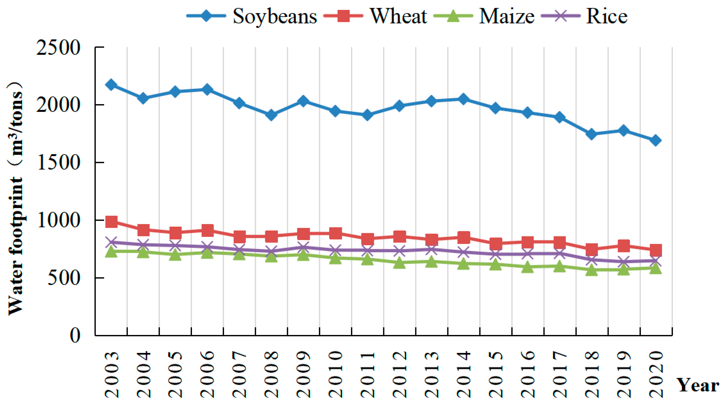
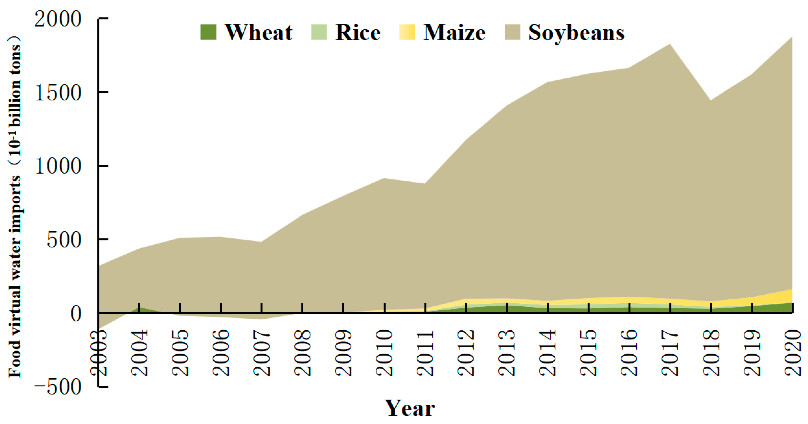
The independent variable is the virtual water in food imports. The virtual water in food imports is measured using the water footprint method, which is applied at the crop level to more precisely capture the water embedded in food production. The water footprint approach accounts for regional and temporal variations in water usage, making it an appropriate tool for analyzing food imports across China’s diverse provinces. Specifically, we focus on the water footprint of four major food crops—rice, wheat, maize, and soybeans—produced in each provincial administrative region of China. Furthermore, the study includes the net imports of animal products, such as pork, beef, lamb, dairy, poultry, and eggs, by converting these imports into crop equivalents. This conversion allows for the integration of animal-based food imports into the virtual water calculation. The net imports of these crops are multiplied by their respective water footprints and the aggregated results provide an estimate of the virtual water content of food imports. This variable serves as an indicator of the virtual water embedded in food imports, reflecting how international trade impacts domestic water resources of food production.
The instrumental variable is China’s food price. This study uses the “Retail Price Index of food Products” to represent “China’s food price” as an instrumental variable. Since “China’s food price” and “food import volume” are closely related and “Virtual water for food imports” is calculated by “the sum of the product of each food import volume and each food virtual water content”. The variable “China’s food price” is theoretically linked to the endogenous variable “virtual water for food imports,” while not being directly influenced by the current random error term or the pressure on water used in food production. As a result, “China’s food price” is selected as the instrumental variable for this analysis (
Table 2).
The control variables are pesticide and fertilizer application, water use structure, irrigation ratio, degree of specialization of crop cultivation, technological environment, and environmental regulation [
37,
39].
2.4. Empirical Modeling of the Effects of Food Imports on Virtual Water Content and the Resulting Water Pressure in Food Production
Given that the data for water pressure in food production (
Fwsi) are censored within the range [0, 1], a Tobit regression model is employed for analysis. The formula is presented as follows:
In Equations (7) and (8), Fwsi*it denotes the dependent variable, reflecting the water pressure from food production in region i during year t. The key independent variable, Fivwit, represents the virtual water associated with food imports in region i for year t. Fivwi(t−1) indicates the first-order lag of virtual water imports. Xz,it represents control variables that capture other factors influencing food production water pressure in region i during year t. Z = 1, 2, …, 6 corresponds to six control variables, namely pesticide and fertilizer application, water use structure, irrigation ratio, crop cultivation specialization, technological environment, and environmental regulation. σ is the constant term of the equation while α represents the coefficient of each variable. μi accounts for the province-specific effects that are not directly observed, φt captures the fixed time effects, and εit is the random error term.
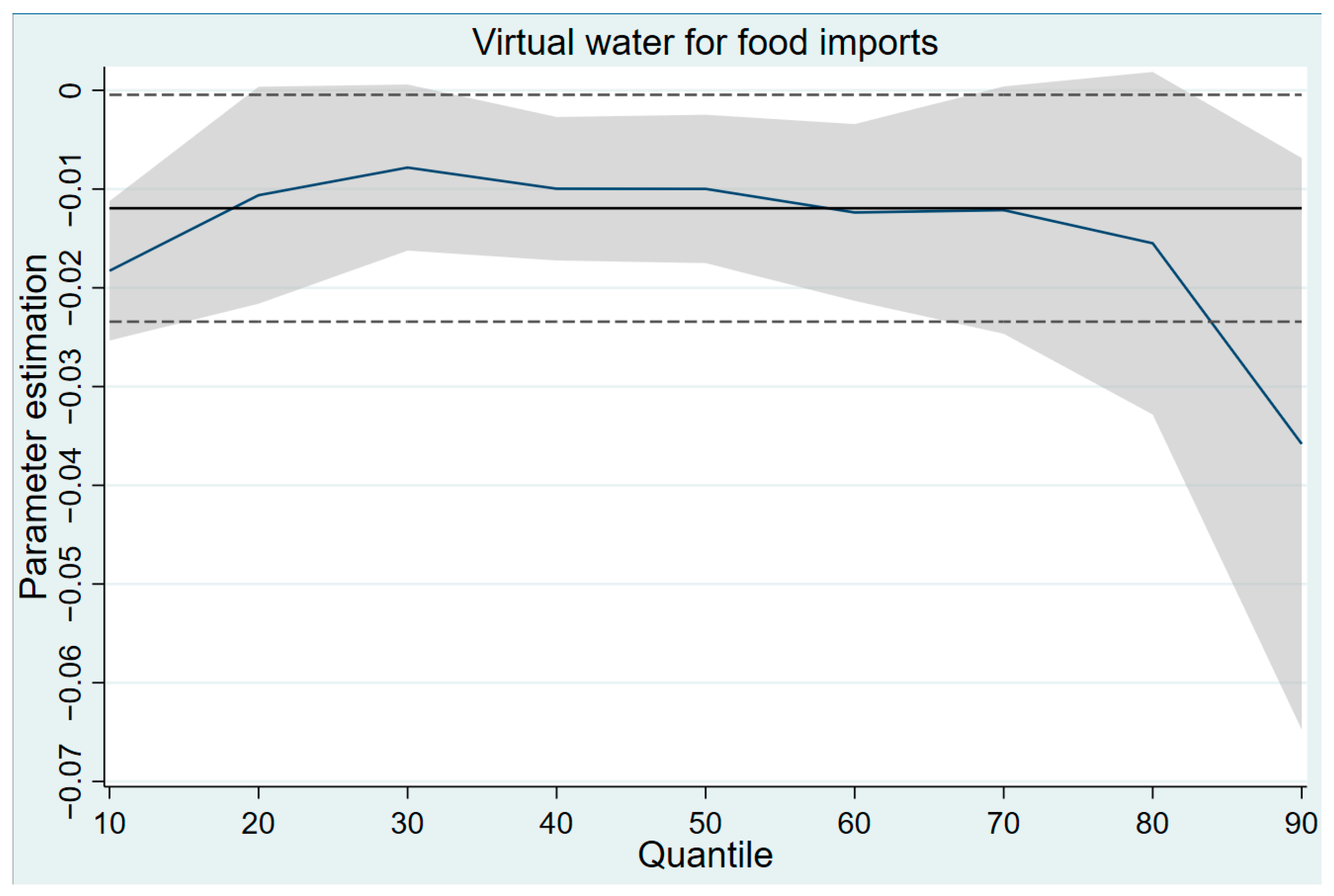
A panel quantile regression model was developed as follows:
In Equation (9), τ represents the quantile, with this study employing quantile regression at intervals of 10%, 20%, …, up to 90%.
Furthermore, spatial econometric modeling is conducted in this research. The global Moran’s I index of water pressure in food production can be expressed as:
In Equation (10), I denotes the index, S2 represents the variance of Fwsi*i, and Fwsi*a signifies the mean of Fwsi*i. Additionally, ωik refers to the spatial distance weighting matrix. The variables n and m denote the total count of provinces in the analysis.
The dynamic spatial panel Durbin model, which examines the effect of virtual water for food imports on the water pressure in food production, is represented by Equations (11) and (12).
where
xl,it represents the value of the
l variable in province
i in year
t,
xl,kt represents the value of the
l variable in province
k in year
t, and
l = 1, 2, …, 7 refers to virtual water for food imports, pesticide and fertilizer application, water use structure, irrigation ratio, crop cultivation specialization, technological environment, and environmental regulation.
ρ is the spatial lag coefficient of water pressure in food production, which indicates the spatial correlation of water pressure in food production among provinces.
Ψ represents the unknown parameter vector of
x, which indicates both the direction and extent of influence each explanatory variable has on regional water pressure in food production.
θ is the spatial lag coefficient for the explanatory variable, reflecting the impact of explanatory variables in neighboring regions on the water pressure in food production in the focal region.
φi denotes the regional fixed effect, while
τt refers to the time-fixed effect, and
εit represents the random disturbance term.
ζ represents the coefficient of this lag term, showing its effect on the current water pressure in food production. This formulation leads to the construction of a dynamic spatial panel Durbin model, allowing for the analysis of both spatial and temporal lag effects of water pressure. This approach provides a more precise estimation of the spatial spillover effects of virtual water for food imports on regional water resource pressures of food production [
14].


