Abstract
Motivation: Breaking through the constraints of water scarcity is a crucial factor for the efficient and sustainable production of food in China. Objective: To explore a new strategy to alleviate the water resource pressure in food production in China, based on the theory of resource flow, this study empirically explores the relationship between food imports and the water pressure in food production in China from the perspective of virtual water trade. Data and Method: This study collects panel data from 30 provincial-level administrative regions in China from 2003 to 2020 and employs methods such as the two-way fixed effects model, instrumental variable approach, and spatial Durbin model for empirical analysis. Results: (1) China’s net food imports surged from −0.000397 billion tons (Bt) in 2003 to 0.118325 Bt in 2020, with a rapid annual growth rate of about 9.37%. Changes in net imports are accompanied by virtual water flows. Between 2003 and 2020, the virtual water content of China’s net food imports increased from 31.7086 Bt to 187.7511 Bt, a yearly increase of 10.39%. (2) Virtual water for food imports has a mitigating effect on the water pressure in food production. Every 0.100 Bt of virtual water imported will reduce the water pressure in food production index by 0.026. The impact has a spatial spillover effect. Moreover, as there is high pressure on water resources in food production in northern regions and major grain-producing areas, the mitigating effect of food imports on the pressure of water resources in food production is also enhanced. The quantile regression found that as the water pressure in food production increases, the mitigating effect of virtual water for food imports on the water pressure in food production gradually increases. Implications: This study examines the relevance of resource flow theory within the context of food trade, thereby broadening the scope of research on virtual water trade in food. Additionally, this study offers valuable insights for the development of strategies aimed at mitigating the pressure on water resources associated with food production in China.
1. Introduction
1.1. Background
Food security is a critical issue for national stability and the well-being of populations, influencing economic, social, and environmental sustainability. Effective management of water resources is essential for securing a stable and reliable food supply, as water plays a central role in agricultural production and food security [1]. In China, water scarcity presents a profound challenge to food security, with per capita water availability standing at just 26% of the global average, highlighting a significant resource constraint [2]. As of 2023, agriculture accounts for approximately 70% of the country’s total water consumption, with food production, in particular, relying heavily on water resources [3]. The spatial distribution of China’s water resources further exacerbates this issue; while about 65% of the nation’s arable land is located in the northern regions, this area holds only 18% of the total water resources [4]. This mismatch between water availability and land cultivation underscores the urgent need for strategies that enhance water-use efficiency in agriculture to ensure sustainable food security.
Additionally, this challenge is compounded by China’s rigid food demand, driven by rapid economic growth, population expansion, and changes in dietary patterns, such as increased meat consumption, which leads to higher feed and water requirements [1]. These pressures, combined with inefficient water usage in agricultural practices, further strain the country’s ability to meet domestic food consumption through local production. As such, the optimization of international food resources has become increasingly critical. China’s reliance on global food markets has risen steadily, emphasizing the importance of food trade in securing its food supply [5].
Given the complexity of these issues, it is important to recognize the broader context of global sustainability frameworks. This paper is directly linked to the United Nations’ Sustainable Development Goal (SDG) 2, which aims to end hunger, achieve food security, improve nutrition, and promote sustainable agriculture. Additionally, SDG 6 on clean water and sanitation is closely related, emphasizing the need for water-use efficiency, particularly in the agricultural sector. The analysis of China’s water–food nexus not only provides insights into its domestic food security challenges but also aligns with global efforts to address sustainable food systems and water management in the face of climate change and population growth.
In terms of study focus, China has been chosen as the primary case due to its unique combination of severe water scarcity, large agricultural sector, and growing integration into global food markets. The study’s findings are expected to offer valuable lessons for other countries facing similar resource constraints, especially in regions with high agricultural dependency and limited water resources.
1.2. Literature Review
As research on virtual resource flow theory continues to deepen, virtual water flow strategies have begun to attract the attention of academia and governments [6]. In response to the growing global scarcity of freshwater and the rising demand for these resources, British scholar Allan introduced the concept of “virtual water” in the 1990s as a means to address issues related to water scarcity and the unequal distribution of water resources across nations. The virtual water strategy has since been recognized as a key approach for optimizing regional water resource allocation and easing the pressure on water resources in various countries and regions. Due to its characteristics of mobility, tradability, and nonmateriality, virtual water is relatively easy and cheap to transport compared to physical water, and is more likely to flow across regions through trade [7]. Furthermore, theoretical studies on virtual water flow can provide insights into the volume of water resources used and the amount of wastewater generated during the production of goods and services across different countries or regions, particularly when viewed from the perspective of global economic trade, and evaluate the benefits of global water resource utilization from a more macroscopic perspective, which can more comprehensively describe the global flow of water resources [8,9,10,11,12,13]. By importing food products from countries or regions with abundant water resources, not only can we help water-poor countries save water but also contribute to the conservation of the world’s total water resources [14]. However, some scholars hold the opposite view. Distefano and Kelly believe that the water-saving benefits of virtual water trade are only effective for relatively wealthy countries, while poor countries or regions have weak economic purchasing power and the corresponding water-saving effect of virtual water trade is therefore weak [15]. Additionally, some scholars have pointed out that the excessive consumption of domestic water resources caused by large-scale food exports will lead to the destruction of the aquatic animal habitat [16].
Moreover, there is already a wealth of research on water resource pressures. Water resource pressures refer to the impact and effect of human beings and socio-economic activities on the use of water resources in a specific natural and social environment that exceeds the capacity of the water environment, thus exerting pressure on the quantity or quality of water [17]. There are four main methods for calculating the water pressure index: the single indicator method, the supply–demand ratio method (Alessa et al., 2008), the strict proportionality method [18], and the comprehensive evaluation method [19]. Of these, the comprehensive evaluation method refers to a type of method that characterizes water resource pressure from multiple perspectives and uses multiple indicators. It mainly includes the water poverty index method [20], the water resource pressure index method, and the comprehensive evaluation of water resource carrying capacity [21]. Among the three measurement methods mentioned above, the comprehensive evaluation method is the most commonly used method for measuring the water resource pressure index, with the water resource pressure index method and the water resource carrying capacity evaluation method being the main methods. Existing methods for calculating the water resource pressure index lack weighting for the differences in endowments between different regions, which reduces the accuracy of the results. At present, 12 of China’s 13 major food-producing provinces have an increasing demand for water resources and the situation is worsening in several resource-rich provinces such as Hebei, Shandong, and Henan. The coupling degree of their water resource distribution and food production is showing a fluctuating downward trend [22,23].
In summary, while trying to quantify the total welfare gains from trade as accurately as possible, scholars are increasingly investigating various potential sources of trade-related welfare. The majority of studies on virtual water in food trade have primarily concentrated on quantifying and analyzing the virtual water flows associated with food imports. Most studies on water pressure in food production also remain in the field of measurement methods and descriptive analysis. However, there are relatively few empirical studies that explore the impact of food trade on water pressure in food production in importing countries. Therefore, this study innovatively explores the mechanism of changes in water pressure in food production in importing countries from the perspective of virtual water of food imports. This study thoroughly examines the relevance of resource flow theory within the context of food trade, thereby extending the scope of research on virtual water trade in food. Additionally, it offers valuable insights for developing strategies aimed at mitigating the strain on water resources associated with food production in China.
1.3. Statement of Research Objectives and Hypotheses
As a typical water-intensive product, the import of food in China has increased in tandem with the rise in total imports. Based on the theory of resource flow, the volume of virtual water imports has also grown accordingly. The virtual water strategy is considered an important measure for optimizing regional water resource allocation and alleviating water stress in different countries and regions. The cross-regional flow of virtual water caused by trade in goods and services essentially transfers water resources spatially through production substitution [24]. International virtual water trade effectively addresses the challenges of long-distance transportation of water resources. By regulating the distribution of water resources, it enables international redistribution of water, providing new ideas for balancing global water resources and ensuring food security. Countries with scarce rainfall, which are already affected by extreme climate events, are experiencing further reductions in precipitation [25]. These water-scarce nations tend to import more water-intensive products to mitigate the obstacles posed by water shortages to their economic and social development.
At the same time, virtual water trade, as a key regulatory mechanism, provides an important avenue for China to quantitatively predict the extent of water scarcity in food production and to plan its agricultural structure rationally [26]. As China’s food trade deficit, particularly in soybean imports, continues to expand, the country, which has relatively limited water resources, imports water-intensive food products from international markets to replenish its virtual water needs. This strategy effectively substitutes for a portion of the water resources required for domestic food production. While promoting trade growth between regions, it significantly alleviates the water stress in China’s water-scarce regions of food production. Based on this, it is hypothesized that food imports can effectively relieve the water pressure on food production in China.
2. Materials and Methods
2.1. Method for Calculating Virtual Water for Food Imports
Virtual water content measurement research is mainly carried out from the following two perspectives. On the one hand, classification is based on virtual water content. There are two main methods. One approach is grounded in the water footprint theory, which assesses the volume of water resources needed for the cultivation of individual agricultural products, thereby providing an estimate of the virtual water trade associated with those products [27]. The other is a method based on input–output data to estimate the amount of virtual water trade in different industries, sectors, and products [5,28]. On the other hand, it is classified according to the perspective of the object and region involved. From the perspective of the object involved, it is mainly focused on the measurement of virtual water in different agricultural products. The measurement of the virtual water content of agricultural products mainly considers climatic factors, soil conditions, crop types, and growth cycles [26,29]. Furthermore, when analyzing the driving forces of virtual water flows, most studies use methods such as gravity models, factor decomposition, and commonality analysis [30,31,32,33,34,35,36].
This study adopts the water footprint method to measure the virtual water content of different domestic food products from the perspective of water demand of food production. Heokstra and Chapagain pointed out that the connotations of virtual water and the water footprint are similar but the water footprint has a wider range of uses [8]. In the context of measuring water usage for crop production, the concepts of water footprint and virtual water are essentially synonymous. The crop water footprint represents the freshwater resources consumed during the production process of crops. Based on the origin of the water used, the crop water footprint can be categorized into two types: the blue water footprint and the green water footprint. This study employs the CROPWAT model, which is endorsed by the Soil Conservation Service of the U.S. Department of Agriculture. By inputting daily climate data from meteorological stations in each provincial administrative region, altitude, latitude, crop coefficients for each crop in different regions, and sowing and harvesting period data, the blue and green water footprints for various crops are computed for each province. The specific formula is as follows:
In Equations (1)–(3), WFP represents the water footprint per unit mass of the crop (m3/kg), with WFPb and WFPg indicating the blue and green water footprints of the crop, respectively (m3/kg). ETg refers to the crop’s green water evapotranspiration (mm) while ETb denotes its blue water evapotranspiration (mm). Y is the crop yield per unit area (kg∙hm−2) and 10 serves as the unit conversion factor. ETc represents the crop’s evapotranspiration (mm), calculated with the Penman–Monteith method as advised by the Food and Agriculture Organization (FAO). Finally, Pe refers to the effective rainfall received during the crop’s growing period (mm).
To facilitate subsequent calculations and empirical analysis, the proportion of feed grains is determined based on internationally recognized feed conversion ratio standards in conjunction with China’s livestock and poultry management practices. Following the approach outlined in Ye and Li [37], imports of beef, lamb, poultry, pork, and dairy products are converted into four major staple grains according to the ratios specified in Table 1. Additionally, employing the aforementioned water footprint methodology, the virtual water content of broadly defined grain imports is estimated.

Table 1.
Broad-based grain conversion ratio.
The virtual water import of i regional crops FWCi (m3) is obtained by summing the water footprints of the quantities of food imported from this region:
In Equation (4), Wbij represents the blue virtual water content per unit of food output, while Wgij denotes the green virtual water content per unit of food output. Yij refers to the net volume of food import trade as most provinces engage in both imports and exports simultaneously. To better understand the actual influence of virtual water for food imports on regional water pressure related to food production, this study refers to net imports of food, i.e., the value of exports minus imports. FWCi indicates the virtual water imported by i regional food crops, replacing the number of water resources required for locally produced food crops, and can therefore be used to represent the virtual water for food imports caused by i regional food imports.
2.2. Method for Calculating Water Pressure in Food Production
The calculation of water pressure in food production mainly combines the single index method with the comprehensive evaluation method. First, with reference to Sun et al. [38], 13 indicators are chosen from four subsystems: water resources, economy, society, and ecology. The entropy weight-TOPSIS method is then applied to assess the water resource carrying capacity of each region. Combined with [39], the index of water pressure in food production can be calculated from the perspective of agricultural water sustainability, which can relatively accurately characterize the variable of water pressure in food production. This is because there are considerable variations in economic, social, and ecological factors across different regions of China. The pressure of water used in food production in different regions is affected not only by water resources endowment but also by economic, social, and ecological factors. Existing studies have only used 40% of water resource endowment to determine whether agricultural water use is sustainable, without considering the impact of economic, social, and ecological factors on regional water resource carrying capacity. This study refers to Li, Li, and Wang [39] and adds the water resource carrying capacity to assign weights to the differences in the four aspects of water resources, economy, society, and ecology in various regions. The ratio of water used in food production to water resource carrying capacity is used to represent the variable of water pressure in food production, which can more realistically, accurately, and reasonably reflect the pressure on various regions caused by water used in food production. The specific calculation method is as follows:
In Formula (5), where Fwsiit indicates the water pressure index of food production in region i in year t; FWCit indicates the amount of water used of food production in region i in year t, and TWCit indicates the total amount of water used in region i in year t; and WRCit indicates the water resource carrying capacity of region i in year t. Water resource carrying capacity (WRC) is calculated using the entropy weight TOPSIS method. For the specific selection of indicators and calculation methods, please refer to Li, Li, and Wang [39].
In Formula (6), GSAit indicates the food sowing area of region i in year t; ASAit indicates the crop sowing area of region i in year t; and AWCit indicates the agricultural water consumption of region i in year t.
2.3. Variable Selection
The dependent variable is water pressure in food production. The selection of the water pressure in food production index is based on a combination of the single index method and the comprehensive evaluation method. Initially, 13 indicators are chosen from water resource, economic, social, and ecological subsystems. These indicators are deemed critical as they represent the multidimensional nature of water pressure on agricultural production. To determine the water resource carrying capacity, we apply the entropy weight-TOPSIS method, which calculates weight coefficients for each indicator, reflecting their relative importance. The water pressure index is then calculated from the perspective of sustainable agricultural water use, offering a more accurate representation of the variable in the context of food production. This approach ensures that the index captures both the quantity and efficiency of water resources used in food production, allowing for a comprehensive assessment of water stress on agriculture across different regions.
The independent variable is the virtual water in food imports. The virtual water in food imports is measured using the water footprint method, which is applied at the crop level to more precisely capture the water embedded in food production. The water footprint approach accounts for regional and temporal variations in water usage, making it an appropriate tool for analyzing food imports across China’s diverse provinces. Specifically, we focus on the water footprint of four major food crops—rice, wheat, maize, and soybeans—produced in each provincial administrative region of China. Furthermore, the study includes the net imports of animal products, such as pork, beef, lamb, dairy, poultry, and eggs, by converting these imports into crop equivalents. This conversion allows for the integration of animal-based food imports into the virtual water calculation. The net imports of these crops are multiplied by their respective water footprints and the aggregated results provide an estimate of the virtual water content of food imports. This variable serves as an indicator of the virtual water embedded in food imports, reflecting how international trade impacts domestic water resources of food production.
The instrumental variable is China’s food price. This study uses the “Retail Price Index of food Products” to represent “China’s food price” as an instrumental variable. Since “China’s food price” and “food import volume” are closely related and “Virtual water for food imports” is calculated by “the sum of the product of each food import volume and each food virtual water content”. The variable “China’s food price” is theoretically linked to the endogenous variable “virtual water for food imports,” while not being directly influenced by the current random error term or the pressure on water used in food production. As a result, “China’s food price” is selected as the instrumental variable for this analysis (Table 2).
Table 2.
Variables and calculation methods of water resource substitution on water pressure in food production.
The control variables are pesticide and fertilizer application, water use structure, irrigation ratio, degree of specialization of crop cultivation, technological environment, and environmental regulation [37,39].
2.4. Empirical Modeling of the Effects of Food Imports on Virtual Water Content and the Resulting Water Pressure in Food Production
Given that the data for water pressure in food production (Fwsi) are censored within the range [0, 1], a Tobit regression model is employed for analysis. The formula is presented as follows:
In Equations (7) and (8), Fwsi*it denotes the dependent variable, reflecting the water pressure from food production in region i during year t. The key independent variable, Fivwit, represents the virtual water associated with food imports in region i for year t. Fivwi(t−1) indicates the first-order lag of virtual water imports. Xz,it represents control variables that capture other factors influencing food production water pressure in region i during year t. Z = 1, 2, …, 6 corresponds to six control variables, namely pesticide and fertilizer application, water use structure, irrigation ratio, crop cultivation specialization, technological environment, and environmental regulation. σ is the constant term of the equation while α represents the coefficient of each variable. μi accounts for the province-specific effects that are not directly observed, φt captures the fixed time effects, and εit is the random error term.
A panel quantile regression model was developed as follows:
In Equation (9), τ represents the quantile, with this study employing quantile regression at intervals of 10%, 20%, …, up to 90%.
Furthermore, spatial econometric modeling is conducted in this research. The global Moran’s I index of water pressure in food production can be expressed as:
In Equation (10), I denotes the index, S2 represents the variance of Fwsi*i, and Fwsi*a signifies the mean of Fwsi*i. Additionally, ωik refers to the spatial distance weighting matrix. The variables n and m denote the total count of provinces in the analysis.
The dynamic spatial panel Durbin model, which examines the effect of virtual water for food imports on the water pressure in food production, is represented by Equations (11) and (12).
where xl,it represents the value of the l variable in province i in year t, xl,kt represents the value of the l variable in province k in year t, and l = 1, 2, …, 7 refers to virtual water for food imports, pesticide and fertilizer application, water use structure, irrigation ratio, crop cultivation specialization, technological environment, and environmental regulation. ρ is the spatial lag coefficient of water pressure in food production, which indicates the spatial correlation of water pressure in food production among provinces. Ψ represents the unknown parameter vector of x, which indicates both the direction and extent of influence each explanatory variable has on regional water pressure in food production. θ is the spatial lag coefficient for the explanatory variable, reflecting the impact of explanatory variables in neighboring regions on the water pressure in food production in the focal region. φi denotes the regional fixed effect, while τt refers to the time-fixed effect, and εit represents the random disturbance term. ζ represents the coefficient of this lag term, showing its effect on the current water pressure in food production. This formulation leads to the construction of a dynamic spatial panel Durbin model, allowing for the analysis of both spatial and temporal lag effects of water pressure. This approach provides a more precise estimation of the spatial spillover effects of virtual water for food imports on regional water resource pressures of food production [14].
2.5. Data Sources and Data Processing
The main data in this study are available from the China Bureau of Statistics, https://www.stats.gov.cn/english/ (accessed on 20 January 2023). The import and export trade data for food products are obtained from the General Administration of Customs of the People’s Republic of China, the Food and Agriculture Organization (FAO) database, and the United Nations Commodity Trade Statistics Database (UN Comtrade). The statistical yearbook data include sources such as the China Statistical Yearbook, the China Rural Statistical Yearbook, the China Water Resources Statistical Yearbook, the China Water Resources Bulletin, the China Agricultural Statistics, the China Environment Yearbook, and the National Agricultural Products Cost and Income Data Compilation. Additionally, the data for key economic indicators are adjusted using the price index, with 2003 serving as the base year.
3. Results
3.1. Results of the Measurement of Virtual Water in China’s Net Food Imports and the Characteristics of Temporal and Spatial Changes
3.1.1. Measurement Results of the Water Footprint of Food Production in China
The water footprint of food production in China from 2003 to 2020 is shown in Table 3. Overall, the water footprint of soybean production in China is the highest, with a national average of 2044.595 cubic meters per ton. The water footprint of maize production is 655.713 cubic meters per ton, about one third that of soybeans. The water footprints of wheat and rice are in the middle, with national averages of 888.94 cubic meters per ton and 741.047 cubic meters per ton, respectively. In terms of regional differences in the water footprint of soybean production, the water footprint of soybean production in the south and southwest regions is at a high level. The Yangtze River’s middle and lower reaches, along with the northeast region, exhibit a moderate level. Regarding regional variations in the water footprint for the production of wheat, maize, and rice, both the South China and the southwest regions show a high level. The northeast and northwest regions are at a lower level. These regional disparities are primarily influenced by factors such as crop coefficients and precipitation during the crops’ growing period.
Table 3.
Water footprint characteristics of four major food production species in different.
Figure 1 illustrates the trends in the national average water footprint of the four primary food productions. Overall, the average water footprint for these four major food items has experienced a consistent decline. This reduction can be attributed to two key factors: firstly, advancements in irrigation technology within food production have progressively decreased the amount of water needed per unit of output. Secondly, the year-over-year enhancements in food production efficiency have led to a reduction in the overall water resources required for each unit of food produced. Among them, wheat decreased from 987.676 cubic meters per ton in 2003 to 739.663 cubic meters per ton in 2020; rice decreased from 806.868 cubic meters per ton in 2003 to 647.073 cubic meters per ton in 2020. Maize decreased from 727.832 m3/t in 2003 to 583.867 m3/t in 2020. The average water footprint of soybeans shows a fluctuating downward trend, decreasing from 2173.334 m3/ton in 2003 to 1910.016 m3/ton in 2008, then rising to 2049.164 m3/ton in 2014, and finally decreasing to 1690.463 m3/ton in 2020.
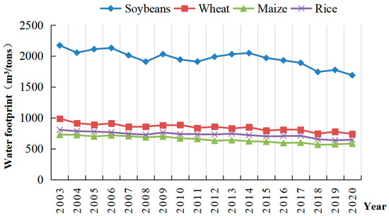
Figure 1.
Water footprint of four main food change characteristics in China during 2003–2020.
3.1.2. Characteristics of Virtual Water Changes in China’s Net Food Imports
Figure 2 shows the characteristics of the change in the scale of virtual water for China’s net food imports from 2003 to 2020. It soared from 31.7086 Bt in 2003 to 187.7511 Bt in 2020, an increase of 492.113%. It can be seen that the amount of virtual water in China’s net food imports is growing rapidly at a rate of about 10.39% per year. Among them, due to the impact of the COVID-19 pandemic, to ensure domestic food security, the amount of virtual water in net food imports in 2020 increased sharply by 15.93% compared to 2019. In addition, there are significant differences in the characteristics of changes in the scale of virtual water net imports.
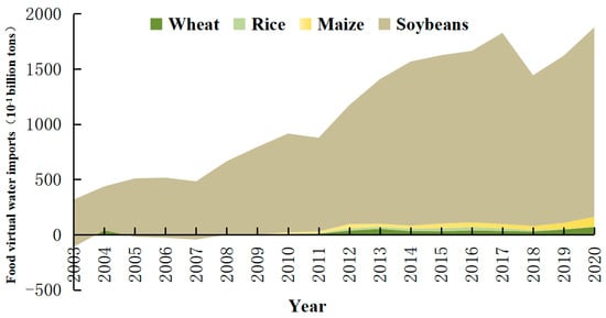
Figure 2.
Food net imports virtual water change characteristics in China during 2003–2020.
First, the scale of virtual water in net wheat imports experienced a trend of first rapidly increasing, then decreasing, and finally slowly increasing. Affected by the large-scale reduction in wheat production in 2003, the virtual water volume of net wheat imports first increased from −1.5877 Bt in 2003 to 5.0204 Bt in 2004, then decreased to −1.9127 Bt in 2007, and finally slowly increased to 6.9249 Bt in 2020. From 2003 to 2020, the total virtual water of net wheat imports increased by 8.5126 Bt. Second, the scale of virtual water for net rice imports shows a trend of rapid increase followed by a slow decrease, gradually increasing from −1.972 Bt in 2003 to 2.0027 Bt in 2012 and then decreasing to 0.2175 Bt in 2020. Third, compared to wheat and rice, the net virtual water imports of maize increased rapidly from −7.6396 Bt in 2003 to 16.5303 Bt in 2020, an increase of 16.5303 Bt in total net virtual water imports. Fourth, soybeans have always been the food product with the largest net virtual water import in China and have grown rapidly from 42.9079 Bt in 2003 to 172.3149 Bt in 2020, an increase of 300.20%.
3.1.3. Regional Differences in Virtual Water in China’s Net Food Imports
As illustrated in Figure 3, notable disparities exist in the virtual water characteristics of net food imports across China’s regions from 2003 to 2020. On the whole, the average virtual water volume of net food imports in the country’s regions experienced a significant upward trajectory, increasing from 1.0146 billion Bt in 2003 to 6.0035 Bt in 2020. Over time, the average virtual water content of net food imports in these regions displayed clear cyclical patterns. Between 2003 and 2007, the average virtual water content fluctuated within a relatively narrow range. However, from 2008 to 2017, a marked acceleration in the virtual water content occurred. In 2018, there was an abrupt decline of 25.11%, followed by a swift recovery and a renewed upward trend.
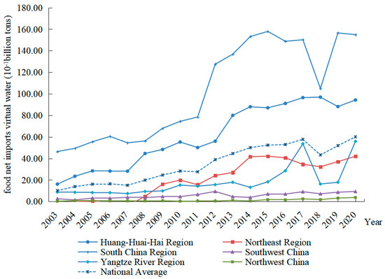
Figure 3.
Regional differences of food net imports virtual water in China during 2003–2020.
The virtual water content of average net food imports varies significantly across different provinces and regions. Firstly, the South China region exhibits the highest virtual water content, demonstrating a fluctuating upward trend. From 2003 to 2014, it grew rapidly from 4.6409 Bt to 8.7976 Bt, reflecting an increase of 444.86%. This was followed by a decline to 10.4931 Bt in 2018 before rising again to 15.4909 Bt in 2020. Secondly, in the Huang-huai-hai region, the average virtual water content of net food imports remains high, with a consistent upward trend. The figure rose sharply from 1.6147 Bt in 2003 to 9.5393 Bt in 2020, an increase of 483.73%. Thirdly, the average virtual water content of net food imports in the northeast and Lower Yangtze regions is classified as moderate. In the northeast, the virtual water content has steadily increased from −1.3223 Bt in 2003 to 4.2049 Bt in 2020. Meanwhile, the Lower Yangtze region has experienced a fluctuating upward trend, rising from 0.8738 Bt in 2003 to 5.5881 Bt in 2020, reflecting a growth of 539.52%, with noticeable declines in 2018 and 2019. Lastly, in the southwest and northwest regions, the average virtual water content of net food imports remains relatively low but both regions show consistent upward trends. In the southwest, the virtual water content increased gradually from 0.2559 Bt in 2003 to 0.9348 Bt in 2020, an increase of 265.33%. Similarly, in the northwest, the figure grew significantly from 0.024.9 Bt in 2003 to 0.3771 Bt in 2020, representing an approximate 14-fold increase.
3.2. The Temporal and Spatial Fluctuations in the Water Pressure in Food Production
Figure 4 illustrates the changes in water pressure in food production in China from 2003 to 2020. For the majority of the samples, the water pressure values fall within the range of 0 to 15. The kernel density function’s distribution curve predominantly displays a pronounced peak with a narrow range. With time, the distribution curve of the kernel density function gradually transitions from an unimodal to a multimodal pattern, indicating that water pressure in food production in China tends to become more extreme due to changes in regional resource endowments and socioeconomic and policy factors. Overall, some of the peaks gradually shifted to the right, even exceeding 40, from 2003 to 2012, and then gradually shifted to the left after 2013, indicating that the overall pressure on water resources in food production in China from 2003 to 2020 showed a trend of first rising and then falling. The reason for this is that as the economic and social levels of the provincial administrative regions continue to develop, so does the water demand, and the ecological water resource system also suffers a certain degree of damage, which leads to increasing pressure on the water used in food production. After 2013, on the one hand, with the implementation of ecological sustainable development policies, the concept of environmental protection and water conservation has taken root, reducing human damage to the ecological water resource system. Additionally, with the increasing import of food, some of the water resources needed to produce food in the importing countries have been replaced. In addition, China’s food production efficiency has been improving year by year, which has resulted in a year-on-year decrease in the amount of water used per unit of food production, thereby alleviating the pressure on water of food production.
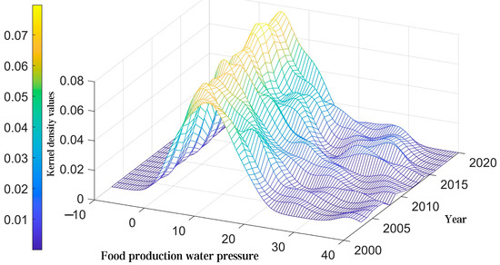
Figure 4.
Estimated kernel density index of water pressure in food production, 2003–2020.
The specific situation of the average water pressure in food production in each region from 2003 to 2020 is shown in Figure 5. Overall, it shows a trend of first increasing and then decreasing but there are significant differences between regions. The Huang-huai-hai region, northwest, and northeast regions show significantly higher levels of water pressure in food production. Among them, Northeastern China and the Huang-huai-hai region account for 44.26% of the country’s cultivated land area and 54.76% of the food sown area with a high demand for water in food production. However, the total water resources in these two regions account for only 9.23% of the national total, i.e., they have low water resources endowment. The mismatch between food production and water resources has led to a long-term high level in the water pressure index in food production in these two regions. In contrast, the pressure on water in food production in South China, Middle and Lower Yangtze, and the southwest regions is significantly lower. Among them, the water pressure index of food production in South China and Southwestern China has long been at a low level due to their high water resource endowment and the fact that the food sown area only accounts for 21.48%, which is at a long-term low level nationwide, resulting in low water demand in food production.
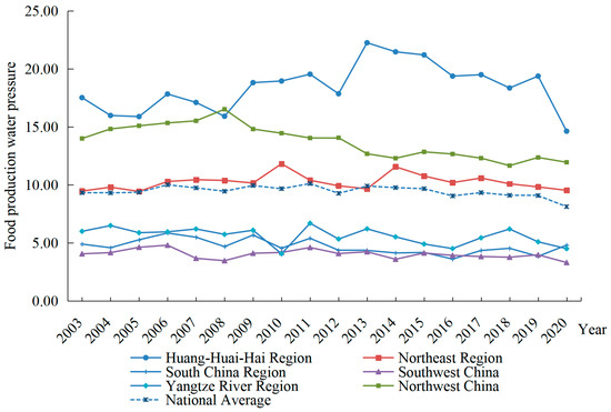
Figure 5.
Water pressure in food production by region, 2003–2020.
3.3. Empirical Analysis of the Impact of Virtual Water for Food Imports on the Water Pressure in Food Production
3.3.1. Baseline Regression Result Analysis
Table 4 presents the estimation outcomes of the model examining the influence of virtual water for food imports on the water pressure in food production. Column (2) reveals a significant impact of virtual water for food imports on water pressure in food production at the p < 1% level, with a coefficient of −0.026. This suggests that an increase of 1 unit in virtual water imports corresponds to a reduction of 0.026 units in the water pressure in food production. By importing a certain amount of food products, the virtual water hidden inside the products is also transferred to various regions of the country, thus partially replacing the water resources needed for domestic food production [40]. This has provided corresponding supplements to areas that were originally relatively scarce in water resources, effectively alleviating the constraints on economic and social development due to scarce resources. While promoting the growth of international trade, it has also greatly alleviated the pressure on water resources for regional food production.
Table 4.
Baseline regression results of the effect of water resources substitution on water pressure in food production.
To address the potential endogeneity within the model, this study employs the instrumental variable approach as a solution to mitigate the endogeneity concerns. The validity of this instrument is first assessed. The regression results presented in column (3) indicate that the F-statistic for the first-stage estimation is 40.01, significantly exceeding the critical value of 10, which suggests that the instrument is not weak. Furthermore, the Wald test for endogeneity is significant at the p < 1% level, confirming that “virtual water for food imports” is indeed endogenous. This supports the use of “China’s food price” as a valid instrumental variable for “virtual water for food imports.” The two-stage regression results reveal that the coefficient for the effect of virtual water for food imports on water pressure in food production is statistically significant at the 5% level, with a value of −0.202, further suggesting that virtual water for food imports plays a role in alleviating the water pressure associated with food production.
Additionally, recognizing that the influence of virtual water for food imports on reducing regional water pressure in food production may not be immediate, a first-order lag term for virtual water imports is incorporated into the regression model. The regression results presented in column (4) reveal that the effect of virtual water imports on food production water pressure is statistically significant at the p < 1% level, with a coefficient of −0.020. This implies that a one-unit increase in virtual water imports leads to a reduction of 0.020 units in the water pressure in food production in the subsequent year. This finding confirms the presence of a time lag in the impact of virtual water for food imports on regional water pressure in food production.
3.3.2. Model Robustness Tests
This study also conducted a series of robustness tests on the impact of virtual water for food imports and water pressure in food production through methods such as replacement estimation and subsample regression.
Replacement Estimation Method
In the empirical analysis examining the influence of virtual water for food imports on the water pressure in food production, the LR test reveals a rejection of the homoscedasticity assumption for the random disturbance term in the panel, indicating the presence of heteroscedasticity. Additionally, the Wooldridge test rejects the assumption of no autocorrelation within groups, signaling the existence of autocorrelation issues. Given that certain provinces or years report zero trade values for food imports, there may be concerns regarding biased estimates in the ordinary panel Tobit model. The results from the PPML, FGLS, and PCSE model tests, presented in columns (1) to (3) of Table 5, demonstrate a significantly negative impact of virtual water for food imports on food production’s water pressure, consistent with the findings of the baseline regression. Moreover, the accuracy of parameter estimation in assessing the impact of virtual water imports on water pressure is contingent upon the correct specification of the parameter model. However, determining the optimal model specification solely through theoretical discussions is challenging. If a nonlinear relationship exists between virtual water imports and water pressure in food production, the model’s regression results may be inaccurate. As a result, to evaluate the robustness of the baseline model, a nonparametric Bootstrap estimation (1000 draws) is performed. The results, shown in column (4) of Table 5, reveal that the effect of virtual water for food imports on water pressure in food production is statistically significant at the p < 1% level, with a coefficient of −0.026. These findings indicate that virtual water imports effectively reduce water pressure in food production, confirming that the baseline model’s regression results are generally robust.
Table 5.
Robustness tests of the effect of water resource substitution on water pressure in food production.
Quantile Regression
To reduce the influence of disturbances, including outliers and error terms, on the estimation results and to ensure a more objective and thorough analysis of how virtual water for food imports influences water pressure in food production across different quantiles, this study applies quantile regression. The quantiles selected range from 10% to 90% as reflected in columns (1) to (9) of Table 6. This approach serves to test the robustness of the baseline regression findings while also exploring the heterogeneity across various regions. The results indicate that although the coefficients and their significance for the impact of virtual water imports on food production’s water pressure vary across quantiles, all coefficients from the 10% to the 90% quantiles remain statistically significant and consistently negative. This suggests that the results from the benchmark regression are robust.
Table 6.
Quantile regression results of the effect of water resources substitution on water pressure in food production.
To more intuitively describe the impact of food imports at different quantiles on water pressure in food production, a quantile regression chart is plotted as shown in Figure 6. At the 10–30% quantile, the impact coefficient of water pressure in food production on food production increases from −0.018 to −0.008. This indicates that in regions with relatively low water pressure in food production (such as the provincial-level administrative regions of Qinghai, Hainan, Chongqing, Guizhou, Sichuan, Yunnan, and Fujian), the mitigating effect of virtual water from water pressure in food production on food production is relatively weak. This is because although these regions partially replace the water resources needed for local food production by importing food products, they have relatively abundant water resources due to their low water demand in food production and high water endowment. Therefore, the water savings have a relatively weak mitigating effect on the water pressure in food production in these regions. At the 30–70% quantile, the coefficient of the impact of virtual water for food imports on pressure on water in food production decreased from −0.008 to −0.012, indicating that in areas with moderate pressure on water in food production (such as the provincial-level administrative regions of Xinjiang, Heilongjiang, Beijing, Gansu, Shaanxi, Jilin, Liaoning, and Anhui), the mitigating effect of virtual water for food imports on the pressure on water of food production is slower. At the 70th to 90th percentile, the impact coefficient of virtual water for food imports on water pressure in food production decreases from −0.012 to −0.036, indicating that in areas with high water pressure in food production (such as the provincial-level administrative regions of Anhui, Henan, Shanxi, Shandong, Tianjin, Hebei, and Ningxia), the mitigating effect of virtual water for food imports on water pressure in food production is stronger. The water demand in food production in these areas is high and the water resource endowment is low, making regional water resources relatively scarce [41]. These areas import food products, which has a stronger effect on the virtual water imported in food production, which is urgently needed for local food production and to a large extent alleviates the pressure on water resources for local food production.
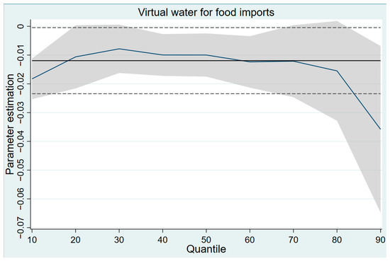
Figure 6.
Plot of quantile regression coefficients of water resource substitution affecting water pressure in food production. Notes: (1) The blue curve in the figure represents the parameter estimates for the virtual water in food imports across various quantiles, derived through quantile regression. (2) The shaded region highlights the 95% confidence interval for these parameter estimates.
3.3.3. Regional Heterogeneity Analysis
North–South Regional Heterogeneity Analysis
To further explore the regional variations in how virtual water for food imports affects water pressure in food production, this study categorizes the samples into northern and southern regions based on their regional characteristics (as presented in Table 7). Columns (2) to (4) demonstrate that whether using the benchmark regression model, incorporating instrumental variables, or adding a first-order lag term for virtual water imports, the results consistently show a significant negative impact of virtual water imports on water pressure in food production. These findings align with the results observed for the full sample. The regression outcomes for the southern region are shown in columns (5) to (8), with column (5) presenting the regression results for the control variables on water pressure in food production. In columns (6) to (8), the regression outcomes all reveal that virtual water imports significantly reduce water pressure in food production.
Table 7.
Heterogeneity in the impact of virtual water imports on water pressure in food production in the north and south.
In general, the regression results for the northern and southern subsamples are consistent with those of the full sample. However, a notable difference is that the impact coefficient of virtual water for food imports on water pressure in food production is significantly higher in the northern region than in the southern region. This suggests that the role of virtual water imports in alleviating water pressure in food production is more pronounced in the north than in the south. The reason for this discrepancy lies in the fact that the northern region has abundant cultivated land resources and the majority of food production in China occurs there, leading to higher water demands for agriculture. Nevertheless, the northern region is characterized by limited water resources and the disparity between the distribution of cultivated land and water resources has resulted in persistent water pressure in food production. As a result, the marginal utility of virtual water imported to reduce water pressure is more substantial in the northern region. Therefore, in comparison to the southern region, virtual water for food imports has played a much more significant role in alleviating water pressure in food production in the northern region.
Heterogeneity Analysis of Grain-Producing Areas
Significant differences may exist in the characteristics of food production between major and nonmajor food-producing regions (Table 8). From columns (2) to (4), the results indicate that regardless of whether the regression is based on the benchmark model, incorporates instrumental variables, or includes a first-order lag term for virtual water imports, virtual water imports consistently exhibit a significant negative effect on water pressure in food production. Apart from the variation in the magnitude of the coefficient, these results align closely with those observed in the full sample regression. The regression outcomes for samples from nonmajor grain-producing areas are shown in columns (5) to (8), where column (5) illustrates the regression results for control variables on water pressure in food production. In columns (6) to (8), the analysis demonstrates that regardless of whether the regression uses the baseline model, includes instrumental variables, or integrates the first-order lag term of virtual water for food imports, the impact of virtual water for food imports on water pressure in food production is found to be insignificant.
Table 8.
Heterogeneity in the effect of water resource substitution on water pressure in food production in different production areas.
The results of the analysis show some variation from those of the full sample regression, suggesting that the impact of virtual water imports on alleviating water pressure for production is significantly more pronounced in major grain-producing areas compared to nonmajor food-producing regions. This disparity can be attributed to several factors. In nonmajor grain-producing areas, the scale of food production is relatively small, resulting in lower water demand. Additionally, these areas are predominantly located in the southern part of China where water resources are abundant and more evenly distributed, leading to a relatively modest initial water pressure in food production. As a result, increases in virtual water imports per unit of food do not significantly affect water pressure in these regions. In contrast, major grain-producing areas are characterized by large-scale, water-intensive production and in some cases, the region faces scarce and unevenly distributed water resources. As such, the water pressure in food production is already substantial, making the impact of increasing virtual water imports more pronounced in these areas.
3.4. Spatial Spillover Effects Across Provinces
In this study, an “inverse distance weighting” matrix was employed to compute the global Moran’s I index for water pressure related to food production across 30 provincial-level administrative regions in China from 2003 to 2020. The findings are presented in Table 9. The spatial autocorrelation coefficients for each year are consistently positive and the significance tests are passed for the majority of the years. These results suggest the presence of spatial autocorrelation in water pressure in food production across the 30 provincial regions analyzed in this study.
Table 9.
Spatially autocorrelated Moran’s I index of water pressure in food production.
To facilitate observation, this study plotted a scatter plot of the spatial distribution of water pressure in food production in 2003, 2009, 2014, and 2019 (Figure 7). From the figure, we can observe that in the sample period, most of the spatially weighted water pressure values in food production in the provinces are located in the first and third quadrants. The results of the fitting analysis also extend across the first and third quadrants, indicating a strong positive global spatial correlation. This suggests the presence of a significant spatial clustering effect regarding water pressure in food production among the 30 provincial-level administrative regions in China from 2003 to 2020. Specifically, provinces with higher water pressure in food production are clustered and provinces with lower water pressure in food production are adjacent to each other, similar to the findings of Deng et al. [9]. This study suggests that incorporating spatial econometric models into the analysis is essential in order to account for spatial effects. This approach would help mitigate measurement bias in models that overlook the influence of geospatial distribution factors.
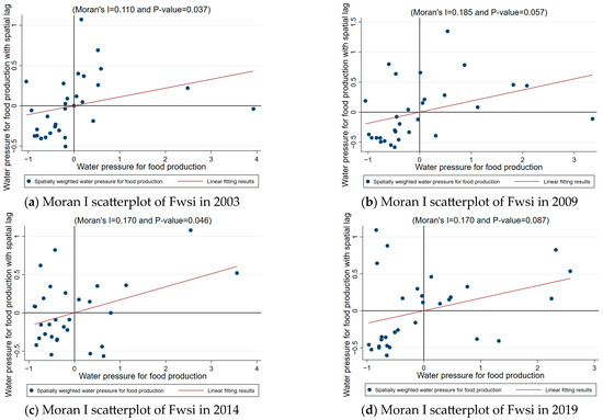
Figure 7.
Scatter plot of Moran’s I index for water pressure in food production in different years.
As shown in column (1) of Table 10, the coefficient for the spatial lag term of water pressure in food production in the dynamic spatial panel Durbin model, calculated using inverse distance weights, is statistically significant at the 1% level, with a value of 0.257. This indicates a positive correlation of water pressure in food production across regions, reinforcing the idea of spatial dependence in water pressure in food production. Furthermore, the coefficient for the food import dummy variable on water pressure in food production is significant at the 1% level, with a value of −0.026. From the results in column (2), it is also observed that the coefficient for the effect of considering the food import dummy for other regions on water pressure in food production in the region is −0.039, which is significant at the 1% level. These findings suggest that the model neglecting spatial effects underestimates the negative impact of food imports on regional water pressure in food production.
Table 10.
A spatial Dubin model of the effect of water resource substitution on water pressure in food production.
Given that the dynamic spatial panel Durbin model is not a linear regression, the coefficients estimated do not provide a direct representation of the marginal effect of virtual water imports on water pressure in food production. To better understand the magnitude of these effects, the coefficients require further decomposition into direct, indirect, and total effects through partial differentiation. Additionally, the dynamic spatial panel Durbin model distinguishes between short-term and long-term effects for each of these three categories, as shown in Table 11.
Table 11.
Decomposition results of spatial spillover effect of water resources substitution on water pressure in food production.
According to the direct effect decomposition results, column (1) reveals that the short-term direct impact of virtual water imports on water pressure in food production is statistically significant at the 1% level, with a coefficient of −0.026. This implies that when accounting for the feedback effect—whereby virtual water imports in a region influence water pressure in food production in neighboring areas, which in turn affects the region’s own water pressure—each 1-unit increase in virtual water imports will result in a reduction of 0.026 units in the region’s water pressure in food production. Column (4) further reveals that after accounting for the feedback effect, the short-term direct influence of virtual water imports on the water pressure in food production remains statistically significant at the 1% level, with a coefficient of −0.035. This implies that a 1-unit increase in virtual water imports leads to a reduction of 0.035 units in the water pressure in food production within the region. These results indicate that the long-term direct impact of virtual water imports on food production water pressure is more substantial than the short-term effect.
The decomposition of indirect effects reveals that, as shown in column (2), the short-term indirect impact of virtual water imports on the water pressure in food production is significant at the 10% level, with a coefficient of −0.035. This indicates that a 1-unit increase in virtual water imports leads to a reduction of 0.035 units in the water pressure in food production in nearby areas. In column (5), the long-term indirect effect of virtual water imports on water pressure is also statistically significant at the 10% level, with a coefficient of −0.046. This suggests that each additional unit of virtual water imported results in a 0.046-unit decrease in the water pressure in food production in neighboring regions. Therefore, the long-term indirect impact on the water pressure in adjacent areas is more substantial than the short-term effect.
The results from the total effect decomposition indicate that, as shown in column (3), the short-term total impact of virtual water imports on food production water pressure is statistically significant at the 1% level, with a coefficient of −0.061. This suggests that a 1-unit increase in virtual water imports leads to a decrease of 0.061 units in the water pressure in food production, both within the region and in its neighboring areas. In column (6), the long-term total effect of virtual water imports on water pressure is also significant at the 1% level, with a coefficient of −0.081. This implies that each additional unit of virtual water imported results in a 0.081-unit reduction in the water pressure in food production, both in the region itself and in surrounding areas. Consequently, the long-term total effect of virtual water imports on water pressure exceeds the short-term effect.
The findings presented above suggest that an increase in virtual water imports for food in a region not only alleviates the water pressure in food production within that region but also reduces the water pressure in adjacent regions. This occurs because, on one hand, water resources are both highly mobile and classified as public goods. As such, they are subject to competition and are nonexclusive, meaning that regions with limited water resources may resort to the continuous exploitation of groundwater and excessive utilization of surface water resources, which to a certain extent take up water resources of neighboring regions, leading to overflow of water pressure in food production to neighboring regions [42]. On the contrary, regions with scarce resources substitute the demand for water in food production by importing food products, reducing the exploitation of groundwater resources and the use of surface water, thus alleviating the pressure on water in food production in the region while reducing the competition for water resources with neighboring provinces.
4. Discussion, Conclusions, Policy Implications, and Limitation
This study examines panel data from 30 provincial-level administrative regions in China, covering the period from 2003 to 2020. The research employs the water footprint approach to assess virtual water associated with food imports and applies the entropy weight-TOPSIS method to evaluate the water resource carrying capacity of each region. Additionally, it calculates the water pressure index of food production from a sustainable agricultural water use perspective. By analyzing the relationship between virtual water imports for food and the water pressure in food production in importing regions, the study reaches the following conclusions: first, the overall water pressure index in food production shows a trend of initially increasing and then decreasing. Notably, the water pressure is significantly higher in the Huang-Huai-Hai region, the northwest, and the northeast. In contrast, regions like South China, the middle and lower reaches of the Yangtze River, and the southwest experience lower levels of pressure. This pattern is consistent with existing studies, which have highlighted regional disparities in water availability and agricultural productivity in China [43]. Second, virtual water imports contribute to mitigating water pressure in food production, demonstrating a food import substitution effect. Specifically, every 0.100 Bt of virtual water imported through food imports reduces the regional water pressure index by 0.026 on average. This effect is accompanied by spatial spillovers, where the virtual water embedded in imported food products is distributed across different regions, effectively substituting domestic water resources needed for local food production. The positive impact of virtual water imports on water resource distribution has been documented in previous studies [44], which emphasize the role of international trade in alleviating local water stress. Further, the study finds that the marginal mitigating effect of virtual water imports is more pronounced in northern regions and major grain-producing areas compared to southern regions and nonmajor grain-producing areas. This is mainly due to the higher water pressure in northern regions and the higher water-use efficiency in key grain-producing areas. This finding aligns with the broader literature on regional water resource disparities and food production dynamics [45]. Lastly, the quantile regression analysis reveals that the impact of virtual water imports on water pressure in food production intensifies as water pressure increases. This highlights the critical role of food imports in managing water scarcity, particularly in areas facing high water stress.
The results of this study provide important insights for addressing water pressure in food production in China and offer actionable policy implications. First, from a research and development (R&D) standpoint, this study recommends increasing government investment in water-efficient and innovative technologies, particularly in regions with high water footprints like South China and Southwestern China. This would help reduce the water required for producing each unit of food in these areas, fostering more sustainable agricultural practices. Second, recognizing regional differences in food imports, particularly in the Huang-Huai-Hai, northwest, and northeast regions, the government should consider increasing food imports from these regions within the constraints of China’s food import tariff quotas. This would maximize the water resource substitution effect, further alleviating water pressure in these water-scarce areas. Third, with regard to food import varieties, ensuring food self-sufficiency while increasing imports, especially of crops like soybeans, could contribute to both water conservation and reduced pressure on domestic agricultural water resources. This strategy would be in line with previous recommendations for balancing domestic production with strategic food imports [46]. This study contributes to practical decision-making by illustrating the potential of virtual water trade to alleviate regional water pressures and provide guidance for stakeholders in government and agriculture. By strengthening R&D in water-efficient technologies, optimizing food import policies, and strategically expanding food imports, China can advance its efforts to achieve sustainable agricultural water use, ensuring food security while managing water resources effectively.
This study has a few general limitations. For instance, it primarily relies on available secondary data, which may not always be perfectly aligned with the most current conditions or capture every aspect of food production and water use. Additionally, the study assumes a consistent relationship between virtual water imports and regional water pressure, which may not hold true in all contexts. While the study covers a broad time span, it does not account for potential short-term fluctuations in agricultural practices or water management policies. Furthermore, the chosen methodology, though robust, might not fully capture the complexities of the relationship between trade and water use in all regions. These limitations suggest that future research could explore more granular data or alternative methodologies.
In light of the study’s findings on China’s food imports, it is crucial to consider the long-term water stress impacts on exporting countries. As China’s demand for water-intensive crops like soybeans, wheat, and maize increases, so does the water footprint of these exports, adding strain to exporting nations’ water resources. Brazil, the largest exporter of soybeans to China, faces significant water stress. Between 2000 and 2020, Brazil’s soybean production nearly doubled to 120 million tons annually. The virtual water embedded in these exports is substantial—about 3000 L per kilogram of soybeans [46]. With China importing around 60% of Brazil’s soybeans, this amounts to approximately 108 billion cubic meters of virtual water annually, which is about 3.6% of Brazil’s total freshwater availability. This increases pressure on water resources in key agricultural regions such as the Cerrado and the Amazon basin. Similarly, Argentina, which exports about 12.4 million tons of soybeans to China, faces water challenges. Its virtual water export is approximately 37 billion cubic meters annually. The country’s reliance on irrigation in regions like the Pampas, combined with over-extraction of groundwater, risks reducing water availability for both domestic use and agriculture. The United States, a major maize exporter to China, also faces challenges. In 2020, U.S. maize exports to China represented an estimated 14.4 billion cubic meters of virtual water. Although the U.S. has more abundant water resources, regional disparities, especially in water-scarce states like California, could affect future agricultural production and exports. These data indicate that as water-intensive agricultural exports to China grow, exporting countries may face increasing water stress, potentially disrupting food supply chains. Sustainable water management strategies are essential to balance both domestic needs and international trade, ensuring long-term stability in global food trade and water use.
Author Contributions
Z.L.: methodology, investigation, writing—original draft. W.Y.: conceptualization, writing—review and editing. C.Z.: proofreads and editing. All authors have read and agreed to the published version of the manuscript.
Funding
The paper is supported by the “Startup Fund for Advanced Talents of Putian University” (grant number: 2024157).
Institutional Review Board Statement
Not applicable.
Data Availability Statement
The data presented in this study are available from the China Bureau of Statistics.
Acknowledgments
The authors would like to thank the anonymous reviewers for their constructive comments and suggestions.
Conflicts of Interest
The authors declare no conflicts of interest.
References
- Huang, F.; Liu, Z.; Ridoutt, B.G.; Huang, J.; Li, B.G. China’s water for food under growing water scarcity. Food Secur. 2015, 7, 933–949. [Google Scholar] [CrossRef]
- Huang, Y.J.; Huang, X.K.; Xie, M.N.; Cheng, W.; Shu, Q. A study on the effects of regional differences on agricultural water resource utilization efficiency using super-efficiency SBM model. Sci. Rep. 2021, 11, 9953. [Google Scholar] [CrossRef]
- Du, T.S.; Kang, S.Z.; Zhang, X.Y.; Zhang, J.H. China’s food security is threatened by the unsustainable use of water resources in North and Northwest China. Food Energy Secur. 2014, 3, 7–18. [Google Scholar] [CrossRef]
- Cai, B.M.; Hubacek, K.; Feng, K.S.; Zhang, W.; Wang, F.; Liu, Y. Tension of Agricultural Land and Water Use in China’s Trade: Tele-Connections, Hidden Drivers and Potential Solutions. Environ. Sci. Technol. 2020, 54, 5365–5375. [Google Scholar] [CrossRef]
- Ali, T.; Huang, J.; Wang, J.; Xie, W. Global footprints of water and land resources through China’s food trade. Glob. Food Secur. 2017, 12, 139–145. [Google Scholar] [CrossRef]
- Taherzadeh, O.; Caro, D. Drivers of water and land use embodied in international soybean trade. J. Clean. Prod. 2019, 223, 83–93. [Google Scholar] [CrossRef]
- Liu, Q.; Lu, R.S.; Lu, Y.; Luong, T.A. Import competition and firm innovation: Evidence from China. J. Dev. Econ. 2021, 151, 102650. [Google Scholar] [CrossRef]
- Chapagain, A.K.; Hoekstra, A.Y.; Savenije, H.H.G. Water saving through international trade of agricultural products. Hydrol. Earth Syst. Sci. 2006, 10, 455–468. [Google Scholar] [CrossRef]
- Deng, J.; Li, C.; Wang, L.; Yu, S.X.; Zhang, X.; Wang, Z. The impact of water scarcity on Chinese inter-provincial virtual water trade. Sustain. Prod. Consum. 2021, 28, 1699–1707. [Google Scholar] [CrossRef]
- Duarte, R.; Pinilla, V.; Serrano, A. Long Term Drivers of Global Virtual Water Trade: A Trade Gravity Approach for 1965–2010. Ecol. Econ. 2019, 156, 318–326. [Google Scholar] [CrossRef]
- Lamastra, L.; Miglietta, P.P.; Toma, P.; De Leo, F.; Massari, S. Virtual water trade of agri-food products: Evidence from italian-chinese relations. Sci. Total Environ. 2017, 599, 474–482. [Google Scholar] [CrossRef] [PubMed]
- Wang, Z.Z.; Zhang, L.L.; Ding, X.L.; Mi, Z.F. Virtual water flow pattern of grain trade and its benefits in China. J. Clean. Prod. 2019, 223, 445–455. [Google Scholar] [CrossRef]
- Delbourg, E.; Dinar, S. The globalization of virtual water flows: Explaining trade patterns of a scarce resource. World Dev. 2020, 131, 104917. [Google Scholar] [CrossRef]
- Zhao, D.D.; Hubacek, K.; Feng, K.S.; Sun, L.X.; Liu, J.G. Explaining virtual water trade: A spatial-temporal analysis of the comparative advantage of land, labor and water in China. Water Res. 2019, 153, 304–314. [Google Scholar] [CrossRef] [PubMed]
- Distefano, T.; Kelly, S. Are we in deep water? Water scarcity and its limits to economic growth. Ecol. Econ. 2017, 142, 130–147. [Google Scholar] [CrossRef]
- O’Bannon, C.; Carr, J.; Seekell, D.A.; D’Odorico, P. Globalization of agricultural pollution due to international trade. Hydrol. Earth Syst. Sci. 2014, 18, 503–510. [Google Scholar] [CrossRef]
- Falkenmark, M.; Widstrand, C. Population and water resources: A delicate balance. Popul. Bull. 1992, 47, 1–36. [Google Scholar]
- Alessa, L.; Kliskey, A.; Lammers, R.; Arp, C.; White, D.; Hinzman, L.; Busey, R. The arctic water resource vulnerability index: An integrated assessment tool for community resilience and vulnerability with respect to freshwater. Environ. Manag. 2008, 42, 523–541. [Google Scholar] [CrossRef]
- Pfister, S.; Koehler, A.; Hellweg, S. Assessing the Environmental Impacts of Freshwater Consumption in LCA. Environ. Sci. Technol. 2009, 43, 4098–4104. [Google Scholar] [CrossRef]
- Garriga, R.G.; Foguet, A.P. Improved Method to Calculate a Water Poverty Index at Local Scale. J. Environ. Eng. 2010, 136, 1287–1298. [Google Scholar] [CrossRef]
- Chen, M.L.; Jin, J.L.; Ning, S.W.; Zhou, Y.L.; Udmale, P. Early Warning Method for Regional Water Resources Carrying Capacity Based on the Logical Curve and Aggregate Warning Index. Int. J. Environ. Res. Public Health 2020, 17, 2206. [Google Scholar] [CrossRef]
- Deng, C.X.; Zhang, G.J.; Li, Z.W.; Li, K. Interprovincial food trade and water resources conservation in China. Sci. Total Environ. 2020, 737, 139651. [Google Scholar] [CrossRef]
- Chen, L.; Chang, J.; Wang, Y.; Guo, A.; Liu, Y.; Wang, Q.; Zhu, Y.; Zhang, Y.; Xie, Z. Disclosing the future food security risk of China based on crop production and water scarcity under diverse socioeconomic and climate scenarios. Sci. Total Environ. 2021, 790, 148110. [Google Scholar] [CrossRef]
- Oki, T.; Kanae, S. Virtual water trade and world water resources. Water Sci. Technol. 2004, 49, 203–209. [Google Scholar] [CrossRef] [PubMed]
- Konar, M.; Dalin, C.; Suweis, S.; Hanasaki, N.; Rinaldo, A.; Rodriguez-Iturbe, I. Water for food: The global virtual water trade network. Water Resour. Res. 2011, 47, 212–223. [Google Scholar] [CrossRef]
- Chen, Z.-M.; Chen, G.Q. Virtual water accounting for the globalized world economy: National water footprint and international virtual water trade. Ecol. Indic. 2013, 28, 142–149. [Google Scholar] [CrossRef]
- Yang, H.; Pfister, S.; Bhaduri, A. Accounting for a scarce resource: Virtual water and water footprint in the global water system. Curr. Opin. Environ. Sustain. 2013, 5, 599–606. [Google Scholar] [CrossRef]
- Masud, M.B.; Wada, Y.; Goss, G.; Faramarzi, M. Global implications of regional grain production through virtual water trade. Sci. Total Environ. 2019, 659, 807–820. [Google Scholar] [CrossRef]
- Yang, H.; Wang, L.; Abbaspour, K.C.; Zehnder, A.J.B. Virtual water trade: An assessment of water use efficiency in the international food trade. Hydrol. Earth Syst. Sci. 2006, 10, 443–454. [Google Scholar] [CrossRef]
- Duarte, R.; Pinilla, V.; Serrano, A. The effect of globalisation on water consumption: A case study of the Spanish virtual water trade, 1849–1935. Ecol. Econ. 2014, 100, 96–105. [Google Scholar] [CrossRef]
- Tuninetti, M.; Tamea, S.; Laio, F.; Ridolfi, L. To trade or not to trade: Link prediction in the virtual water network. Adv. Water Resour. 2017, 110, 528–537. [Google Scholar] [CrossRef]
- Dalin, C.; Konar, M.; Hanasaki, N.; Rinaldo, A.; Rodriguez-Iturbe, I. Evolution of the global virtual water trade network. Proc. Natl. Acad. Sci. USA 2012, 109, 8353. [Google Scholar] [CrossRef]
- Dalin, C.; Hanasaki, N.; Qiu, H.G.; Mauzerall, D.L.; Rodriguez-Iturbe, I. Water resources transfers through Chinese interprovincial and foreign food trade. Proc. Natl. Acad. Sci. USA 2014, 111, 9774–9779. [Google Scholar] [CrossRef] [PubMed]
- Shao, L.; Guan, D.B.; Wu, Z.; Wang, P.S.; Chen, G.Q. Multi-scale input-output analysis of consumption-based water resources: Method and application. J. Clean. Prod. 2017, 164, 338–346. [Google Scholar] [CrossRef]
- Liu, J.; Sun, S.K.; Wu, P.T.; Wang, Y.B.; Zhao, X.N. Inter-county virtual water flows of the Hetao irrigation district, China: A new perspective for water scarcity. J. Arid Environ. 2015, 119, 31–40. [Google Scholar] [CrossRef]
- Zhuo, L.; Mekonnen, M.M.; Hoekstra, A.Y. Consumptive water footprint and virtual water trade scenarios for China—With a focus on crop production, consumption and trade. Environ. Int. 2016, 94, 211–223. [Google Scholar] [CrossRef]
- Ye, W.; Li, Z. Will the Grain Imports Competition Effect Reverse Land Green Efficiency of Grain Production? Analysis Based on Virtual Land Trade Perspective. Agriculture 2023, 13, 2220. [Google Scholar] [CrossRef]
- Sun, L.Y.; Miao, C.L.; Yang, L. Ecological-economic efficiency evaluation of green technology innovation in strategic emerging industries based on entropy weighted TOPSIS method. Ecol. Indic. 2017, 73, 554–558. [Google Scholar] [CrossRef]
- Li, Z.Q.; Li, X.Y.; Wang, Y.J. Does Decentralized Food Crop Cultivation Threaten Water-Land-Food Nexus? A Spatial Econometric Analysis. Water 2023, 15, 1096. [Google Scholar] [CrossRef]
- Yawson, D.O. Estimating virtual water and land use transfers associated with future food supply: A scalable food balance approach. MethodsX 2020, 7, 100811. [Google Scholar] [CrossRef]
- Maroufpoor, S.; Bozorg-Haddad, O.; Maroufpoor, E.; Gerbens-Leenes, P.W.; Loaiciga, H.A.; Savic, D.; Singh, V.P. Optimal virtual water flows for improved food security in water-scarce countries. Sci. Rep. 2021, 11, 21027. [Google Scholar] [CrossRef] [PubMed]
- Sun, C.Z.; Zhao, L.S.; Zou, W.; Zheng, D.F. Water resource utilization efficiency and spatial spillover effects in China. J. Geogr. Sci. 2014, 24, 771–788. [Google Scholar] [CrossRef]
- Liu, J.; Zehnder, A.J.B.; Yang, H. Historical Trends in China’s Virtual Water Trade. Water Int. 2007, 32, 78–90. [Google Scholar] [CrossRef]
- Cai, B.M.; Feng, K.S.; Zhang, W.; Liu, Y.; Wang, F.; Hubacek, K. Mitigating trade-driven water scarcity via water-saving irrigation in China: Different role of surface water and groundwater. Resour. Conserv. Recycl. 2024, 205, 107570. [Google Scholar] [CrossRef]
- Zhang, Z.Y.; Yang, H.; Shi, M.J. Spatial and sectoral characteristics of China’s international and interregional virtual water flows—Based on multi-regional input-output model. Econ. Syst. Res. 2016, 28, 362–382. [Google Scholar] [CrossRef]
- Woertz, E. Virtual water, international relations and the new geopolitics of food. Water Int. 2022, 47, 1108–1117. [Google Scholar] [CrossRef]
Disclaimer/Publisher’s Note: The statements, opinions and data contained in all publications are solely those of the individual author(s) and contributor(s) and not of MDPI and/or the editor(s). MDPI and/or the editor(s) disclaim responsibility for any injury to people or property resulting from any ideas, methods, instructions or products referred to in the content. |
© 2025 by the authors. Licensee MDPI, Basel, Switzerland. This article is an open access article distributed under the terms and conditions of the Creative Commons Attribution (CC BY) license (https://creativecommons.org/licenses/by/4.0/).