Study on the Estimation of Greenhouse Sensible Heat Flux Based on the Surface Renewal Method: Validation and Calculation Results

Abstract

To address the issues of poor universality, high cost, and difficulty in parameter acquisition associated with existing methods for estimating crop evapotranspiration (ET_c) in greenhouses, this study focused on tomato plants in a Venlo-type greenhouse (Zhenjiang, Jiangsu Province, from 20 November 2024 to 9 January 2025) to explore the applicability of the surface renewal (SR) method in greenhouses. Micrometeorological data were collected by deploying high-frequency temperature sensors and other equipment. The accuracy of sensible heat flux (H) estimation by the traditional Snyder method and the Chen method was compared. Based on the latent heat flux (LE) measured by the evaporimeter method, the actual sensible heat flux was derived through an energy balance model, which was then used for comparative verification with the estimation results of the two methods. The results showed that the Chen method, which incorporates friction velocity (u*) and does not rely on the empirical calibration coefficient α, is adaptable to the characteristics of non-uniform airflow in greenhouses. Under sunny conditions (R² = 0.722 during the day and R² = 0.712 at night) and cloudy conditions (R² = 0.7558 during the day and R² = 0.754 at night), the estimation accuracy of the Chen method was significantly higher than that of the Snyder method. Moreover, for the entire experimental period, the R² value reached 0.733, the Pearson’s r coefficient was 0.856, and the outlier rate was as low as 9.1%. This study innovatively applies the SR method to semi-closed heated greenhouses, making a clear distinction from previous SR studies conducted in open-field environments and providing a new approach for the accurate estimation of greenhouse heat flux.

1. Introduction

The crop evapotranspiration (ET_c) in greenhouses is a key parameter for crop water management and environmental regulation. The accurate estimation of ET_c is of great significance for optimizing irrigation regimes and improving crop yield and quality [1,2,3]. Currently, the commonly used methods for estimating greenhouse evapotranspiration (ET) can be mainly divided into three categories: non-mechanistic models, such as ET models combining greenhouse meteorological characteristics and crop factors; direct measurement methods [4], such as lysimeters, runoff meters, and eddy covariance systems; and mechanistic models, which are widely applied and based on canopy transpiration, leaf energy balance, or the processes of mass and energy exchange between crops and air. Among these, at present, mechanistic models improved based on the Penman–Monteith (P-M) model theory are the most commonly used methods for estimating greenhouse crop ET [5,6,7,8,9].

In the field of estimating evapotranspiration (ET) of greenhouse crops, the model system can be divided into two major categories: statistical models and mechanistic models. Statistical models belong to empirical evapotranspiration (ET) models dominated by meteorological factors, which specifically include multiple linear regression models, artificial neural network (ANN) models, Hargreaves models, and so on. For example, multiple linear regression models estimate ET by performing linear fitting on meteorological factors such as solar radiation and air temperature, and they are simple and efficient in regions where the linear correlation of data is strong. Artificial neural network models can capture the complex nonlinear relationships between ET and meteorological factors, and have better estimation accuracy in scenarios involving multi-factor interactions. Hargreaves models only require temperature data for calculation—though easy to apply, their parameters need to be modified according to regional characteristics in humid areas or areas with high wind speeds. These models do not involve crop physiological processes nor the in-depth interaction mechanisms of the “crop–atmosphere–soil” system, and their core lies in fitting the variation patterns of ET using meteorological observation data, where the weights of driving variables such as solar radiation (Rn), temperature (T_a), and relative humidity (RH) need to be determined based on regional meteorological characteristics (e.g., the proportion of diffuse radiation in high-latitude regions and the diurnal variation law of vapor pressure deficit (VPD) in humid regions) [10,11,12,13]. Taking the ET estimation of greenhouse tomatoes as an example, when such models are applied across regions, they are affected by differences in climate, greenhouse structure, crop variety, and layout between the two regions, so parameters such as leaf area index (LAI), canopy height (H), and VPD threshold need to be remeasured and calibrated [14], and due to the simplification of processes such as canopy turbulent exchange, and the coupling of photosynthesis and root water uptake, these models have poor universality and require extensive parameter calibration under different scenarios [15,16]; mechanistic models are constructed based on the intrinsic mechanisms of crop physiology, energy balance, or material exchange, and mainly include two types of models: one is the photosynthetic physiology-driven ET models, whose core parameters (e.g., stomatal conductance response parameters gs₀ and gs_max) are derived based on the mechanism of crop photosynthetic carbon assimilation and the laws of growth stages, rather than relying solely on data fitting [17,18], among which stomatal conductance is regulated by the crop growth stage and the temperature–humidity environment—for instance, under high-temperature or drought conditions, stomatal conductance decreases significantly, which in turn affects the ET rate; the other is the comprehensive physical process-based ET models, with the Penman–Monteith model as a typical representative, whose accurate ET estimation relies on the acquisition of complex parameters such as canopy resistance and stomatal conductance [19,20,21], where canopy resistance fluctuates with changes in LAI during the crop growth stage, differences in greenhouse ventilation, and variations in canopy structure, while the dynamic change in stomatal conductance is closely coupled with photosynthetic physiological processes, and the difficulty in obtaining such parameters limits the practical applicability of the model; although direct measurement methods (e.g., lysimeters, runoff meters) achieve high accuracy in ET estimation, they suffer from high sensor costs and a high operational threshold, requiring professional personnel for installation, debugging, and maintenance, and also having strict requirements for the soil quality of the installation site [22], which makes it difficult for most research institutions and small-scale growers to afford and use them effectively in practical promotion; in summary, there is an urgent need for a new method with wide universality, high cost-effectiveness, and relatively good accuracy for ET estimation of greenhouse crops.

To address the aforementioned limitations of existing ET_c estimation methods, this study intends to take sensible heat flux as the breakthrough point, and adopts the SR method to achieve the accurate quantification of sensible heat flux—thereby providing a reliable basis for deriving ET_c through the energy balance equation. As an emerging method for evapotranspiration estimation, the SR method relies less on parameters and has better adaptability compared with traditional classic energy balance-based methods (such as the Bowen Ratio–Energy Balance method, BREB, and the eddy covariance method, EC) and the classic Penman–Monteith meteorological model. It demonstrates significant application potential for sensible heat flux calculation. For the calculation method of the SR method, please refer to Section 2.3. Paw U et al. used a high-frequency (10 Hz) temperature sensor as the scalar for describing surface renewal, and regarded the ramp-like changes in the time series as the dominant feature for analyzing the moisture and heat exchange between the ground surface and air. Their study found that the accuracy of sensible heat flux calculated based on the surface renewal theory was extremely high [23,24,25]. Liu et al. [26] extended the application of the SR method to a semi-enclosed banana orchard covered with plastic film, verifying that this method can still achieve high accuracy in sensible heat flux estimation under such passively ventilated and unregulated environmental conditions. However, there is an essential difference between this scenario and the fully enclosed, actively heated winter greenhouses studied in this paper: Josef’s research only considered natural energy inputs (e.g., solar radiation) in the orchard’s energy balance, with no involvement of any artificial interventions. In contrast, in winter greenhouses, artificial heat flux (accounting for 5–10% of the total energy input in cold regions) and airflow disturbances caused by forced ventilation are core influencing factors of the energy balance, which directly determine the partitioning patterns of sensible and latent heat fluxes. The traditional SR method has not been designed to calculate or discuss such artificial intervention scenarios, making it unable to fully characterize the energy balance characteristics of winter greenhouses. The direct application of the traditional SR method may lead to insufficient accuracy in heat flux estimation, which has become a key technical barrier to the promotion of this method in greenhouse systems.

Aiming at the problems in evapotranspiration estimation of crops in Venlo-type greenhouses—where traditional energy balance models (e.g., the eddy covariance method) suffer from sensible heat flux distortion due to turbulent disorder in enclosed environments, and empirical models (e.g., the Penman–Monteith model) have insufficient universality as they rely on crop parameters and complete meteorological data [27,28,29,30,31]. Targeting the characteristics of non-uniform airflow and artificial regulation in winter closed heated greenhouses, this study breaks through the traditional application boundary of the SR method that assumes “uniform airflow in open spaces” [32]. It explores the applicability of the SR method in semi-closed environments and establishes an SR estimation process adapted to heating scenarios. This study provides a low-cost quantitative tool for greenhouse precision irrigation, offers support for the accurate estimation of greenhouse evapotranspiration, and expands the application boundary of the surface renewal method.

2. Materials and Methods

2.1. Study Site and Climate

This experiment was conducted in Dagang District, Zhenjiang City, Jiangsu Province, China (32.181441° N, 119.629464° E), at an altitude of 18.5 m. This region has a mild subtropical climate, with an average annual precipitation of 1029.1 mm, an average annual temperature of 15.5 °C, and an average annual reference evapotranspiration of 892.24 mm. Precipitation is mainly concentrated from April to October, accounting for 80% of the annual total precipitation. The average annual relative humidity is 76%, the annual cumulative sunshine duration is 2051.7 h, the frost-free period is 239 days, and the average annual wind speed is 3.4 m/s. The research target was a Venlo-type greenhouse, with a length of 35.2 m, a width of 25.2 m, an eave height of 6 m, and a gutter height of 5.5 m. The greenhouse used 4 mm thick float glass as the covering material, which has a light transmittance of approximately 95%, a heat transfer efficiency of 2%, and anti-condensation performance. During the experimental testing period, the test plants in the greenhouse were tomatoes. This experiment ran from 20 November 2024, to 9 January 2025, and the average outdoor temperature during this period ranged from 8 °C to 18 °C.

2.2. Micrometeorological Data Collection

As shown in Figure 1, the surface renewal observation system comprises the following equipment with their corresponding measurement accuracies: the CR1000X data logger (CR1000X, Campbell Scientific, USA), with a voltage signal measurement accuracy of ±0.02% FS, a temperature measurement accuracy of ±0.01 °C, and a sampling accuracy of up to 0.1 μV; an air temperature and humidity sensor (SM6395B, Sonbest, China), with a temperature accuracy of ±0.2 °C (0–65 °C) and a relative humidity accuracy of ±3% RH (10–90% RH, non-condensing); a net radiation sensor (JTBQ-2, TINEL, CHINA), with a sensitivity of 7–14 μV·W⁻¹·m² and a measurement accuracy of ±5% under standard radiation conditions; a wind speed sensor (W410C2, Chwvn, China), with a measurement range of 0–60 m/s, an accuracy of ±0.3 m/s in the 0–10 m/s range, and an accuracy of ±3% of the reading in the 10–60 m/s range; a high-frequency thermocouple (Type E, Omega, China), with a temperature measurement range of −200–900 °C, an accuracy of ±0.5 °C in the 0–400 °C range, an accuracy of ±1% of the reading above 400 °C, and a response time of ≤10 ms; a soil heat flux plate (SN-3001-TR-SHF-N01, Renke, China), with a measurement range of −500–500 W/m², an accuracy of ±3% FS, and a linearity error of ≤±2%; an evaporimeter (J16021, Chwvn China), with an evaporation capacity measurement accuracy of ±0.1 mm and a resolution of 0.01 mm; and an electronic balance (ST, Faya, China), with a maximum capacity of 5000 g, a readability of 0.01 g, and a repeatability error of ≤±0.02 g.

$$R_n^{\prime }=R_n+Q_h$$

(1)

$$R_{\mathrm{n}}^{\prime }=H+LE+G$$

(2)

The high-frequency temperature sensor was installed 1 m above the tomato canopy to measure temperature (T). The net radiation sensor was mounted 1.5 m above the canopy to measure the net radiation (R_n) above the greenhouse canopy. The energy input (Q_h) of the heating system is calculated based on the temperature difference between the inlet and outlet water, $Q_h=P\times \eta \times \mathrm{t}\times 3600$; in this equation, P represents the rated power of the heating equipment, $\eta$ represents the thermal efficiency of the heating system, and t represents the cumulative operating time of the heating system during the study period (h). The net solar radiation (R_n) and artificial heating energy (Q_h) are combined into the total net radiation (R_n′). The anemometer was placed at a height of 1 m (consistent with that of the high-frequency temperature sensor) to measure wind speed (u). The soil heat flux sensor was buried 5 cm deep in the soil beneath the canopy to measure the surface soil heat flux (G). H represents the sensible heat flux, and LE represents the latent heat flux. The sampling frequency for high-frequency temperature and wind speed was set to 10 Hz, while the sampling frequency of other sensors was set to 1 min.

2.3. Dynamic Changes in Heat Flux in the Greenhouse

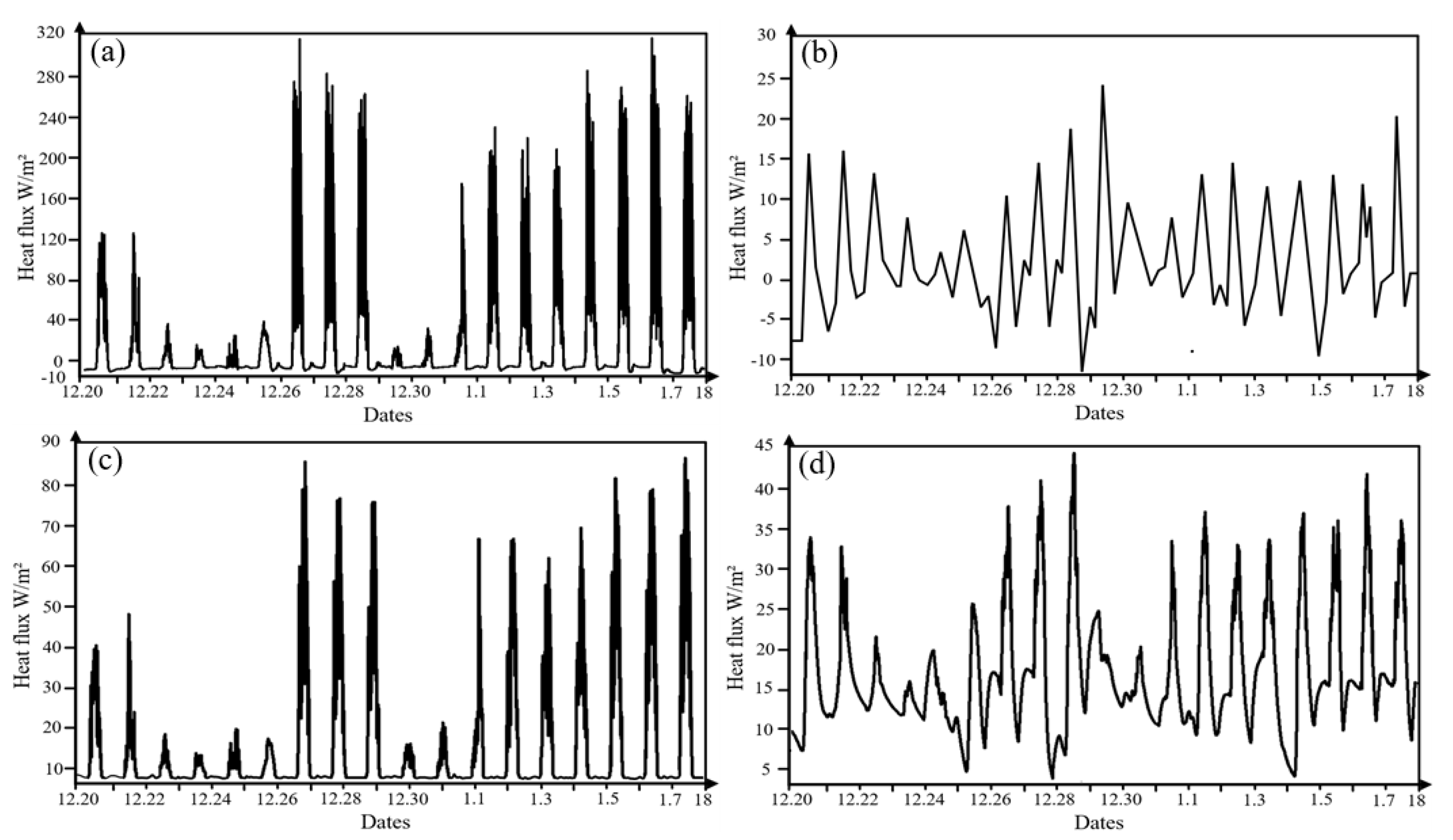
Figure 2a–c show the actual data of net radiation, soil heat flux, latent heat flux, and sensible heat flux in the greenhouse from 20 December 2024 to 9 January 2025, respectively. On sunny days in the greenhouse, the maximum values of net radiation, soil heat flux, and latent heat flux are 288 W/m², 20 W/m², and 100 W/m², respectively, while their minimum values are −13.5 W/m², −10 W/m², and 30 W/m², respectively.

Based on the measured heat flux data (as shown in Figure 2a–d) and combined with the heat balance model, the sensible heat flux in the greenhouse from 20 December 2024 to 8 January 2025 was estimated (as shown in Figure 2d). The calculation results show that the sensible heat flux in the greenhouse varies significantly in different time periods. During the daytime, due to sufficient solar radiation and a large temperature difference, the sensible heat flux reaches a maximum value of 45 W/m², which occurs on sunny days and relatively warm daytime periods. In these periods, the large temperature difference between the inside and outside of the greenhouse promotes the effective exchange of sensible heat.

However, at night, due to the operation of the heating system in the greenhouse, the temperature inside the greenhouse is effectively maintained, and the sensible heat flux shows a significant recovery during the nighttime greenhouse heating period. There is a large difference between the nighttime temperature recovery inside the greenhouse and the ambient temperature. During this period, the sensible heat flux is usually maintained between 10 W/m² and 20 W/m², with the minimum value dropping to 5 W/m². This phenomenon reflects that the heating system increases the greenhouse temperature, leading to a significant recovery of the temperature difference between the inside and outside of the greenhouse, which enhances the intensity of heat exchange between the inside and outside of the greenhouse. At the same time, the continuous energy supply from the internal heating system further increases the sensible heat flux.

In general, the estimation results of sensible heat flux based on the heat balance model show that the sensible heat flux in the greenhouse reaches a maximum value of 45 W/m² during sunny daytime, while it drops to a minimum of 5 W/m² at night due to the reduced temperature difference.

In this experiment, to evaluate the transpiration of tomato crops, the evaporation pan method was employed, with conversion performed according to the evaporation coefficient (K_c = 1.7) for the mature stage of tomatoes specified by the Food and Agriculture Organization (FAO). The potential uncertainties of this validation mainly stem from two aspects: first, the difference between the evaporation from the evaporator’s exposed water surface and crop transpiration (affected by canopy structure and stomatal regulation), and second, the spatiotemporal variability of the K_c coefficient (influenced by temperature, humidity, ventilation, etc.). To reduce errors, this study adopted three optimizations: (1) placing the evaporator in the middle of the greenhouse canopy to simulate the microclimate; (2) slightly revising the K_c coefficient (±5%) based on daily meteorological data; and (3) recording every 2 h to reduce the accumulation of instantaneous errors. It is estimated that the overall error is controlled within ±8%, meeting the relevant acceptable range. In specific calculations, when converting ET_c to LE, the formula used was as follows:

$$LE={\displaystyle \frac{L_e·E{T}_{\mathrm{c}}}{M}}$$

(3)

In the equation, LE represents the latent heat flux (W·m⁻²); ET_c denotes the transpiration rate (kg·m⁻²·s⁻¹); L_e is the latent heat of vaporization of water (2.45 × 10⁶ J·kg⁻¹); and M is the mass of transpired water per unit area per unit time (kg·m⁻²·s⁻¹).

This formula converts transpiration into latent heat flux, reflecting the energy exchange involved in water evaporation during the transpiration process. This experiment was conducted from 20 November 2024 to 9 January 2025, which coincided with the mature stage of tomatoes. The measurements of transpiration and latent heat flux of tomatoes in the greenhouse provided basic data for the further analysis of water and energy exchange processes.

2.4. Calculation of H Using the Surface Renewal Method

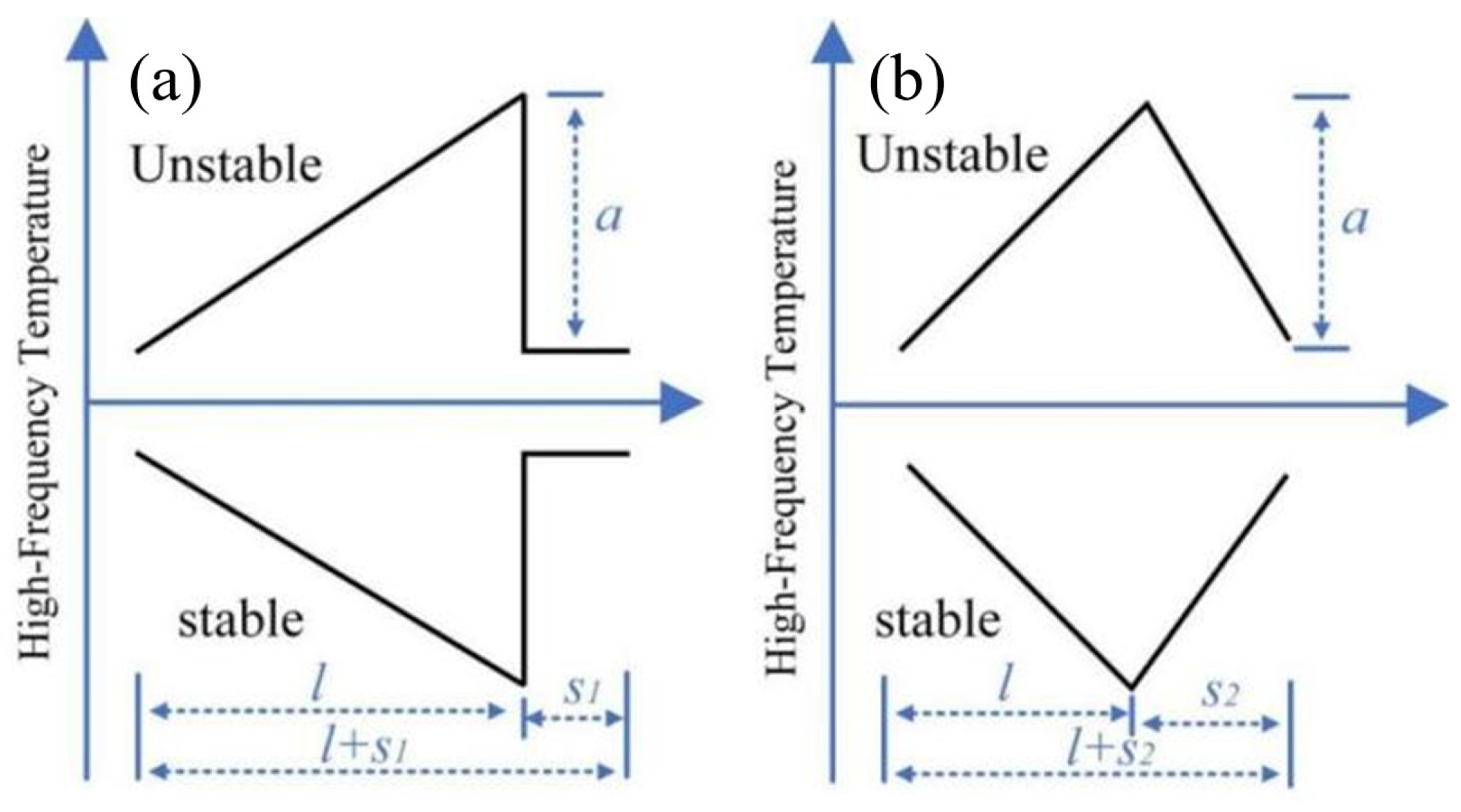
When an air mass sweeps across the ground surface, if the temperature of the upper air is lower than that of the air near the ground (indicating instability), the high-frequency temperature data drop rapidly. This is followed by a stable period (s), and then an unstable period (l), during which the ground surface heats the air mass and the temperature rises gradually. Typically, within a few seconds, the warm air mass is ejected upward and replaced by the colder air mass above [33], as illustrated in Figure 3a. Under stable and unstable atmospheric conditions, the temperature gradient is characterized by amplitude (a) and the frequency of reverse slopes (l + s), as shown in Figure 4b.

Therefore, the average sensible heat flux (H_SR) at a specific observation height (z) and within a designated observation period (e.g., 30 min) represents the net heat exchange of all ramp events during that time period. The mathematical expression for sensible heat flux can be derived using the following formula [34]:

$$H_{SR}=\rho C_p{\displaystyle \frac{\mathrm{d}T}{\mathrm{d}t}}{\displaystyle \frac{V}{A}}$$

(4)

In this equation, ρ and Cp represent air density (g·m⁻³) and specific heat capacity at constant pressure (J·g⁻¹·K⁻¹), respectively; dT/dt denotes the temperature change rate (K·s⁻¹); under the assumption of neglecting the advection effect, V/A represents the air volume per unit area below the observation point; this ratio converts the volumetric heating rate (W·m⁻³) into the sensible heat flux density (W·m⁻²), and its value is proportional to the observation height z.

Due to the step-like changes in high-frequency temperature observations at or above the crop canopy (as shown in Figure 3b), the term dT/dt can be approximated by the average temperature change rate over the entire step period (typically 30 min). Therefore, Equation (1) can be simplified to the following form [34]:

$$H_{SR}=\rho C_p{\displaystyle \frac{a}{l+s}}(\alpha z)=\rho C_p{\displaystyle \frac{a}{\tau }}(\alpha z)$$

(5)

In this equation, α describes the uniformity of heating within a unit volume of air, where α = 1 indicates that all air is uniformly heated; z denotes the observation height of the high-frequency temperature sensor; τ is the period of step changes, which equals the sum of the duration of temperature step changes (or heating time, l) and the static period during which temperature remains constant (s). Both a and τ can be determined using the temperature structure function Sⁿ(r) proposed by van Atta [34]. Among them, the calculation of a is relatively complex because it requires solving the real root of a cubic equation, i.e., Equation (3) [35].

$${T_a}^3+pa+q=0$$

(6)

$$p=10S^2\left(r\right)-{\displaystyle \frac{S^5\left(r\right)}{S^3\left(r\right)}}$$

(7)

$$q=10S^3\left(r\right)$$

(8)

$$S^n\left(r\right)={\displaystyle \frac{1}{m-j}}{{\displaystyle \sum _{i=1+j}^m(T_i-T_{i-j})}}^n$$

(9)

$$\tau =-{\displaystyle \frac{r{a}^3}{S^3(r)}}$$

(10)

In this equation, T_i is the temperature value at time i; j is the lag time of high-frequency temperature sampling; T_i−j is the temperature value at time i−j; r is the ratio of the time lag j to the temperature observation frequency; m is the number of high-frequency temperature observation data points within the entire step cycle; n is the power of the temperature structure function, which can generally take values of 2, 3, or 5.

2.5. Calculation of H Using the Improved Surface Renewal Method

Hu et al. [36] argued that the theoretical model of temperature change proposed by Paw U et al. is overly idealized. In reality, there is no sudden and significant drop in temperature before the ramp heating, nor is there a static period during which the temperature remains constant. Instead, after reaching the maximum value, the temperature rapidly changes from a high value to a low value, forming a limited microfront, as shown in Figure 4. Based on the decomposition of temperature observation data into random and coherent components [30], they proposed to calculate a and τ in Equation (7) using the maximum sampling delay during the microfront and the friction velocity (u^∗).

$${\displaystyle \frac{a}{{\tau }^{\frac{1}{3}}}}=-\gamma {[{\displaystyle \frac{S^3(r_m)}{r_m}}]}^{{\displaystyle \frac{1}{3}}}$$

(11)

$$\begin{array}{c}{\displaystyle \frac{1}{\tau }}=\left\{{\displaystyle \frac{\beta \frac{u_{*}}{h}}{\beta \frac{u_{*}}{\mathrm{z}-d}}}\right.\end{array}\begin{array}{c}\\ \end{array}\begin{array}{c}\\ \end{array}{\displaystyle \frac{0.2h<z\le h+2(h-d)}{z\le 0.2h\mathrm{or}\mathrm{z}>h+2(h-d)}}$$

(12)

In this equation, S³(r) represents the temperature structure function of the third order. The sampling lag, r_m, is the value that maximizes $-{[S^3(r)/r]}^{{\displaystyle \frac{1}{3}}}$. The correction factor γ is used to adjust the difference between $a/{\tau }^{{\displaystyle \frac{1}{3}}}$ and the maximum value of $-{[S^3(r)/r]}^{{\displaystyle \frac{1}{3}}}$ [36]. The height of the canopy is denoted as h, while d refers to the zero-plane displacement height, typically two-thirds of h. Additionally, β is another correction factor, used to correct the difference between ${\displaystyle \frac{1}{\tau }}$ and ${\displaystyle \frac{u_{*}}{h}}$ [or ${\displaystyle \frac{u_{*}}{z-d}}$] [36].

By substituting Equations (8) and (9) into Equation (2), we obtain the following equation:

$$H_{SR}=\{{\displaystyle \frac{-\alpha {\beta }^{\frac{2}{3}}\gamma \rho C_p{[\frac{S^3(r_m)}{r_m}]}^{\frac{1}{3}}{u}_{*}^{\frac{2}{3}}\frac{z}{h^{\frac{2}{3}}}}{-\alpha {\beta }^{\frac{2}{3}}\gamma \rho C_p{[\frac{S^3(r_m)}{r_m}]}^{\frac{1}{3}}{u}_{*}^{\frac{2}{3}}\frac{z}{{(z-d)}^{\frac{2}{3}}}}}{\displaystyle \frac{0.2h<z\le h+2(h-d)}{\mathrm{z}\le 0.2h\mathrm{or}\mathrm{z}>\mathrm{h}+2(h-d)}}$$

(13)

In this equation, the coefficients α, β, and γ can be determined based on observational data [36]. Although their values vary across different surfaces (such as Pinus strobus, crop residues, and bare soil), their product is approximately 0.4, and the differences between different surfaces are generally negligible [37]. Therefore, this product can be treated as a constant in applications.

Early studies by Paw U et al. and Chen et al. provided a theoretical basis for calculating sensible heat flux using the high-frequency temperature method, establishing a classical approach centered on the temperature structure function. This work laid the theoretical and methodological foundation for estimating latent heat flux (transpiration) via the energy balance residual method.

2.6. Evaluation Criteria

The coefficient of determination (R²) (Equation (12)) [38], Pearson’s coefficient (Equation (13)) [38], root mean square error (RMSE) (Equation (14)) [38], and mean absolute error (MAE) (Equation (15)) [38] were used as evaluation indicators to statistically analyze the accuracy of latent heat flux calculated by the SR method.

$$R^2=1-{\displaystyle \frac{{\displaystyle \sum _i^n{\left(Y_i-\widehat{Y_i}\right)}^2}}{{\displaystyle \sum _i^n{\left(Y_i-\overline{Y}\right)}^2}}}$$

(14)

$${pearson}^{\prime }s={\displaystyle \frac{\sum (x-\overline{x})(y-\overline{y})}{\sqrt{\sum (x-\overline{x}{)}^2}\times \sqrt{\sum (y-\overline{y}{)}^2}}}$$

(15)

$$RMSE={\displaystyle \frac{1}{n}}{{\displaystyle \sum _{i=1}^n(y_i-{\hat{y}}_i)}}^2$$

(16)

$$MAE={\displaystyle \frac{1}{n}}{\displaystyle \sum _{i=1}^n(y_i-{\hat{y}}_i)}$$

(17)

x_i and y_i represent the latent heat fluxes calculated by the SR method and the evaporation pan method, respectively; i is the sample size; and $\overline{y}$ and ${\stackrel{\wedge }{y}}_i$ denote the estimated comparison value via least squares regression and the mean value of the standard values, respectively.

3. Results and Analysis

Evaluation of Two SR Models

This study focuses on the accuracy of two surface renewal methods (the Snyder method and the Chen method) in estimating the sensible heat flux in greenhouses. A comparative study was conducted via correlation analysis: the performance of the two methods was compared against the actual sensible heat flux (Hₒ) under different weather conditions (sunny days and cloudy days), while also considering the influence mechanisms of human interventions such as greenhouse ventilation (during daytime) and nighttime heating. The results are as follows:

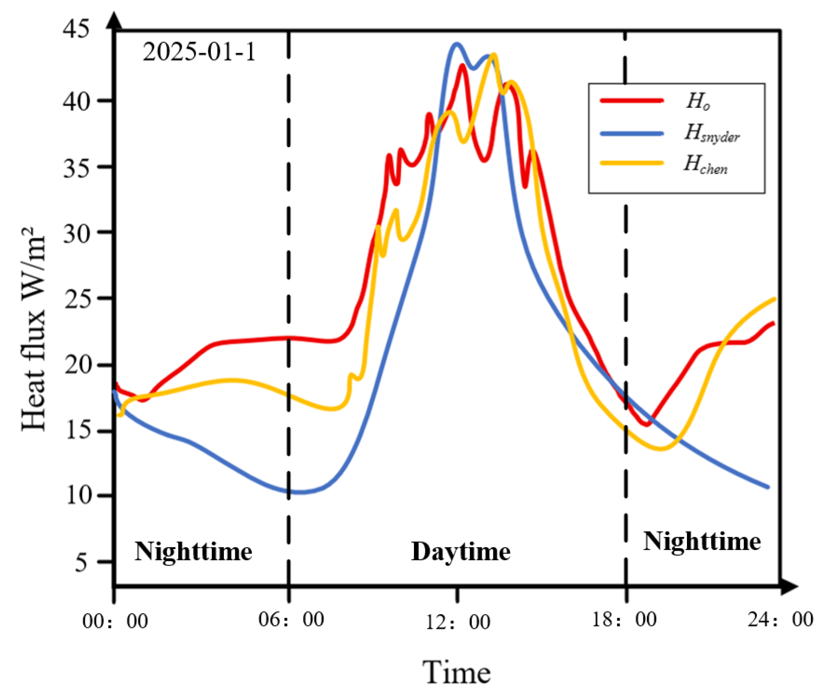
As shown in Figure 5, under sunny daytime conditions when the greenhouse heating system is not in operation, solar radiation is the main factor driving changes in sensible heat flux. The sensible heat flux estimated by the Chen method (H_chen) can accurately match the actually measured sensible heat flux (Hₒ) both in terms of peak magnitude and the timing of peak occurrence. This is because the Chen method incorporates the concept of friction velocity (u*), fully accounts for the turbulent exchange process at the vegetation–atmosphere interface within the greenhouse, and avoids the independent use of the calibration coefficient (α)—all of which contribute to the higher accuracy of the sensible heat flux calculated by the SR_chen method. In contrast, the sensible heat flux estimated by the Snyder method (H_snyder) deviates significantly from the actual Hₒ. This discrepancy may be attributed to two key limitations of the Snyder method: first, it does not introduce the concept of friction velocity; second, it assumes that air masses throughout the greenhouse are uniformly heated. However, due to disturbances from greenhouse fans and the opening of skylights, the temperature of air masses inside the greenhouse is actually non-uniform. Additionally, the Snyder method uses an empirical calibration coefficient (α = 0.5) [39], and the lack of empirical relationships for calibration coefficients specific to greenhouse environments further leads to significant deviations between the estimated and actual sensible heat fluxes. During sunny nights when the greenhouse heating system is activated, the heated air rises. This, combined with the temperature inversion near the glass surfaces in the greenhouse, jointly drives the generation of corresponding friction velocity. As mentioned earlier, the Chen method incorporates friction velocity and does not require the separate determination of the calibration coefficient (α), enabling it to still accurately capture the sensible heat flux in the greenhouse environment during nighttime heating. Similarly, the Snyder method fails to account for the non-uniform heating of the entire fluid mass and requires the independent determination of α, resulting in a significant deviation of H_snyder from the actual Hₒ and a noticeable underestimation.

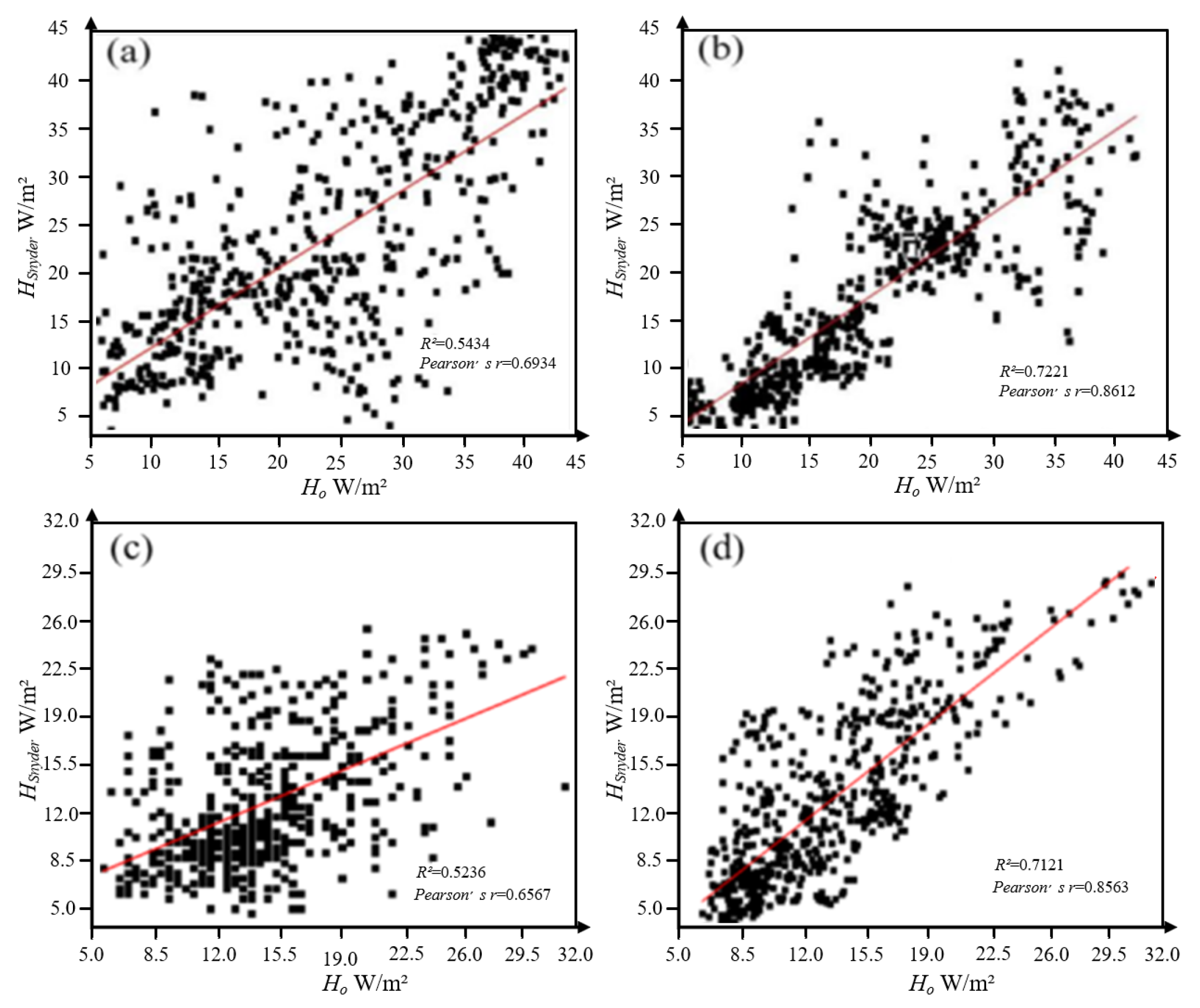
As shown in Figure 6a,b, under sunny daytime conditions, the coefficient of determination (R² = 0.7221) and Pearson correlation coefficient (r = 0.8612) between H_chen and H_ₒ are much higher than those between H_snyder and H_ₒ (R² = 0.5434, Pearson’s r = 0.6934). This indicates that, under sunny daytime conditions with high solar radiation and the greenhouse heating system turned off, the Chen method can more accurately estimate the sensible heat flux in the greenhouse environment. As shown in Figure 6c,d, the coefficient of determination (R² = 0.7221) and Pearson correlation coefficient (r = 0.8563) between H_chen and H_ₒ remain at relatively high levels during sunny nights. In contrast, the corresponding values for H_snyder and H_ₒ are R² = 0.5258 and Pearson’s r = 0.6567. These results further demonstrate that the Chen method can accurately calculate the sensible heat flux in the greenhouse both during daytime (with ventilation) and nighttime (with artificial heating) under sunny conditions.

As shown in Figure 7, under cloudy conditions, solar radiation is blocked by clouds during the daytime, leading to a significant reduction in sensible heat flux with gentle variations. H_chen still closely follows the changes in H_ₒ. This is because, as radiation decreases, the transpiration rate of plants is greatly reduced; although transpiration is reduced, friction velocity still exists inside the greenhouse due to the operation of internal fans and the opening of skylights. This explains why the Chen method can still accurately calculate the sensible heat flux in the greenhouse even when plant transpiration is low on cloudy days. There is a large error between H_snyder and H_ₒ, which is attributed to the fact that the Snyder method lacks important data on turbulent exchange inside the greenhouse, resulting in a significant deviation between the calculated sensible heat flux and the measured value. During nighttime greenhouse heating, the trend consistency between H_chen and H_ₒ is stronger, while the consistency between H_snyder and H_ₒ is poor. This phenomenon is basically the same as that observed on sunny nights, and the underlying reason is also identical.

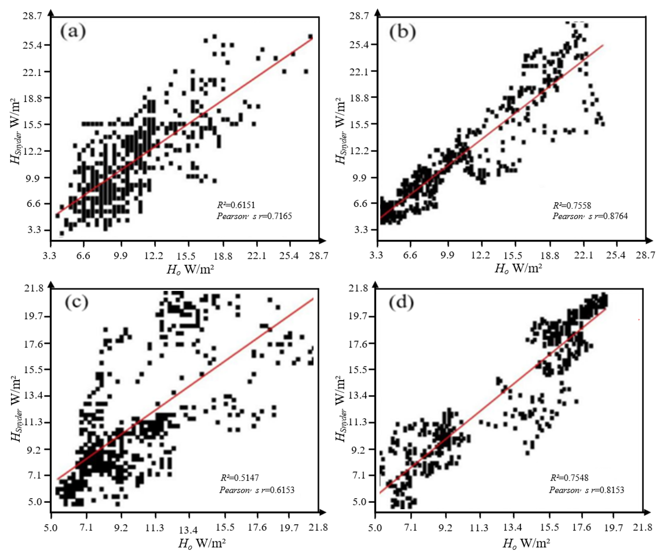
As shown in Figure 8a,b, under cloudy daytime conditions, the coefficient of determination (R² = 0.7558) and Pearson correlation coefficient (r = 0.8764) between H_chen and H_ₒ are higher than those between H_snyder and H_ₒ (R² = 0.6151, Pearson’s r = 0.7655). This indicates that, on cloudy days, even with low solar radiation and no greenhouse heating during the daytime, the Chen method still maintains high reliability in estimating sensible heat flux. As illustrated in Figure 8c,d, the coefficient of determination (R² = 0.7548) and Pearson correlation coefficient (r = 0.8153) between H_chen and H_ₒ remain at relatively high levels at night, which are significantly higher than those between H_snyder and H_ₒ (R² = 0.6147, Pearson’s r = 0.6153). This further verifies the accuracy of the Chen method in calculating sensible heat flux in the greenhouse both during daytime and nighttime under cloudy conditions.

By synthesizing the analysis results under two weather conditions (sunny and cloudy days) and two typical greenhouse operating conditions (no heating during daytime and heating at nighttime), it can be concluded that the Chen method, by introducing friction velocity and avoiding reliance on the empirical calibration coefficient α, is physically compatible with the sensible heat transfer characteristics of greenhouses under different operating conditions. Its estimation accuracy and stability are significantly superior to those of the Snyder method. Therefore, the Chen method is more suitable for estimating sensible heat flux in greenhouse environments.

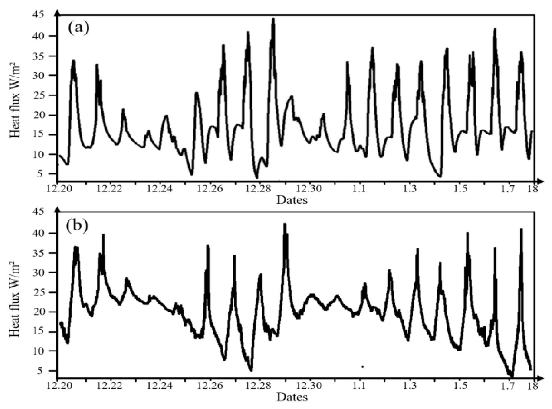
The previous study found that the sensible heat flux calculated by H_chen is more accurate than that calculated by H_snyder under different weather conditions [40]. To accurately describe the overall simulation effect of greenhouse sensible heat flux, this study used the Chen method to conduct a comparative verification of sensible heat flux throughout the entire test period, as shown in Figure 9. When the dynamic changes in flux are significant—especially at the moment when the weather suddenly changes from sunny to cloudy—H_chen can track the jump changes in flux in a more timely manner and more accurately. Its dynamic response capability is far higher than that of the sensible heat flux calculated by the Snyder method, providing reliable data support for the calculation of greenhouse sensible heat flux under complex weather conditions.

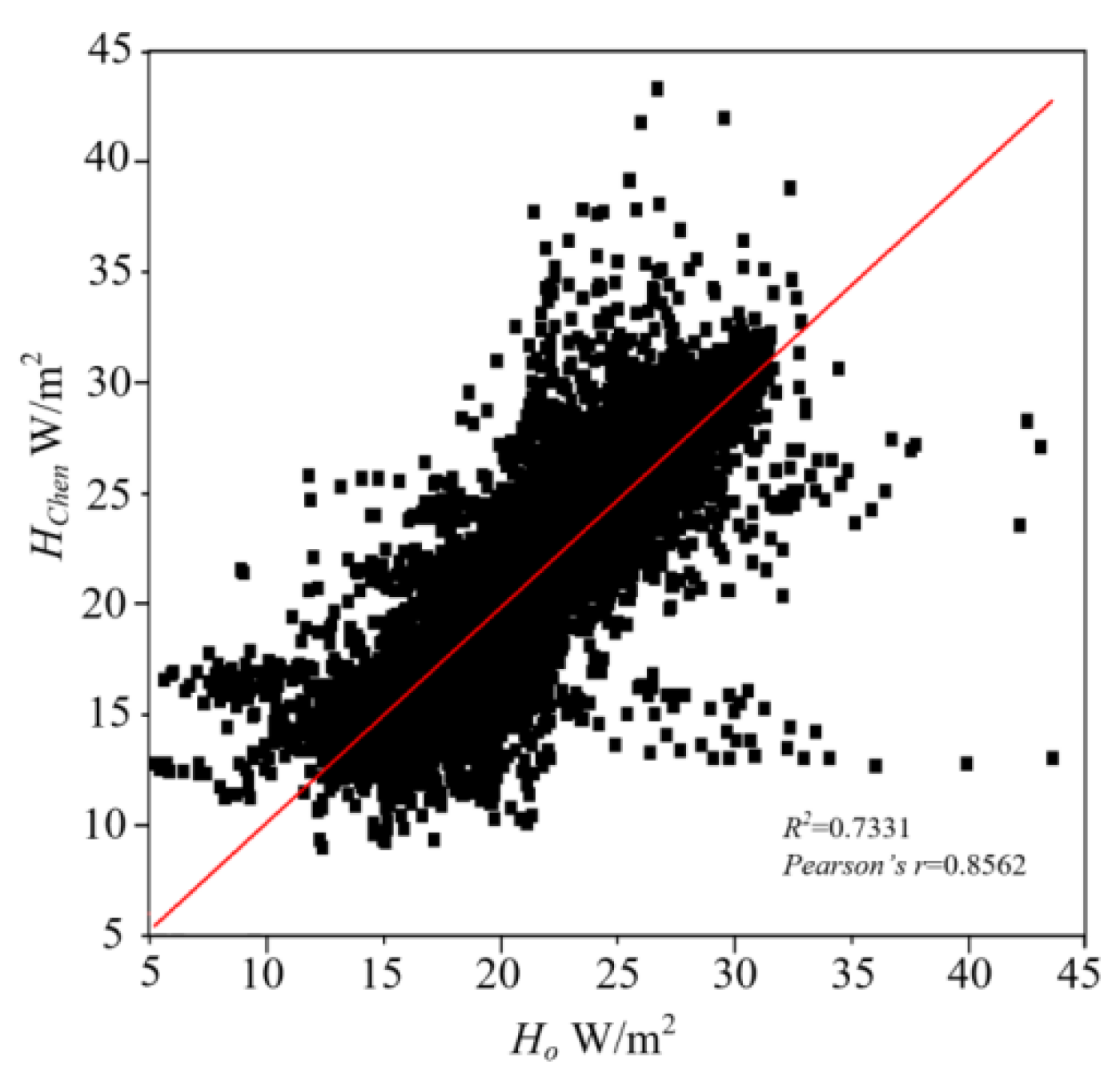
Figure 10 shows the correlation analysis between the actual greenhouse sensible heat flux (H_ₒ) and the sensible heat flux calculated by the Chen method (H_chen) throughout the entire test period. From the perspective of correlation analysis, the sensible heat flux calculated by the Chen method has a strong correlation with the actual sensible heat flux, with a Pearson’s correlation coefficient of 0.8562 and an R² value of 0.7331. This indicates a significant linear relationship between the two types of fluxes. This result is highly consistent with the conclusions of correlation analysis under different weather conditions (R² = 0.7221 for sunny days, R² = 0.7558 for cloudy days, and R² = 0.8153 for nighttime). From a statistical perspective, it verifies the stable performance of the Chen method across multiple scenarios and the entire time period. Unaffected by weather conditions or artificial environmental interventions, the Chen method can be used to estimate sensible heat flux in all-weather human-controlled environments.

4. Discussion

As a technique for calculating sensible heat flux based on high-frequency temperature data, the SR method is mostly limited to application in open and fully exposed farmland ecosystems [23,24,25]. Its underlying assumption is that the airflow over the underlying surface of open farmland is uniform and free from any artificial disturbances. This study is the first to introduce the SR method into a semi-open Venlo-type glass greenhouse. Equipped with a forced ventilation system and a nighttime low-temperature heating system, this greenhouse represents a complex environment where “artificial regulation and natural exchange” are coupled. This attempt provides a new perspective and method for estimating sensible heat flux in greenhouses.

Although the enclosed structure and artificial regulation measures of Venlo-type greenhouses have altered the water vapor transfer law in traditionally open spaces, they have precisely created a favorable environment for the stable operation of high-frequency temperature sensors. This is because the glass-covered greenhouse isolates external interferences such as low temperature, frost, and precipitation. Meanwhile, the nighttime heating system maintains the greenhouse environment at night, reducing the impact of extreme low temperatures on the sensitivity of high-frequency temperature sensors and avoiding “dead spots” in measured data caused by condensation or icing [41]. This is relatively consistent with the conclusion of Wu et al. [42] in their study on temperature sensor stability, which states that “regulating temperature can reduce the abnormal rate of temperature sensors by approximately 60%”.

Due to the complex environmental and mechanical structures of Venlo-type greenhouses, the internal airflow field remains in a non-uniform state for extended periods. During the daytime, the opening of skylights and fan ventilation create a state of “horizontal ventilation and vertical convection” inside the greenhouse [43]. At night, the heating system located on the greenhouse floor causes heated air to rise, forming a vertical circulation with the temperature inversion layer near the glass [44]. This non-uniform airflow completely invalidates the assumption of the Snyder method, which presupposes that air masses are under uniform heating conditions. In contrast, by introducing the concept of friction velocity, the Chen method effectively adapts to the characteristics of turbulent exchange within the greenhouse. It quantifies the intensity of airflow disturbance inside the greenhouse (e.g., u* = 0.15 m/s when fans are operating, and u* = 0.05 m/s in the non-ventilated state) and reflects the turbulent mixing efficiency at the vegetation–atmosphere interface of the greenhouse. This is highly consistent with the physical mechanism of energy transfer in greenhouses and serves as a crucial indicator for describing energy transfer in non-uniform airflow. In contrast, the Snyder method does not account for friction velocity and relies solely on the empirical calibration coefficient α = 0.5 [39]. However, in the greenhouse of this study, the calibration coefficient α ranges from 0.7 to 1.4 (calculated via H_ₒ inversion) due to fan disturbances and heating. This discrepancy inevitably leads to deviations in the sensible heat flux calculated by the Snyder method, which is consistent with the finding of Hu et al. [40] that the error in sensible heat flux calculated using the Snyder method in tea plantations increases by approximately 35%. Meanwhile, when using the Snyder method to estimate sensible heat flux, it is necessary to solve a cubic equation individually for each H value. If the data results are unstable, the third-order temperature structure function is highly likely to approach zero. Since l + s serves as the denominator in Equation 2, this will cause abnormal points (outliers) in the calculated results [45]. In contrast, the Chen method eliminates the need to solve cubic equations and does not use the third-order temperature structure function (l + s) as a denominator. This method significantly reduces the occurrence of abnormal points in calculation results, decreasing the abnormal point rate from 30.5% (1220 out of 4000 total samples) to 9.1% (364 out of 4000 total samples). The uncertainty of the outlier rate was quantified using the binomial proportion confidence interval (95% CI: ±1.8% for the Snyder method and ±0.9% for the Chen method), confirming the statistical significance of the reduction. Additionally, the Chen method increases the calculation speed by more than three times [46].

To better quantify model accuracy (as suggested), we supplemented two key evaluation metrics—root mean square error (RMSE) and mean absolute error (MAE)—to complement R² and Pearson’s r. Under sunny conditions during the daytime with forced ventilation (maximum solar radiation reaching 288 W/m², the dominant driver of sensible heat flux changes), the Chen method achieved an R² of 0.722, RMSE of 18.6 W/m², and MAE of 14.3 W/m², while the Snyder method yielded an R² of 0.543, RMSE of 27.9 W/m², and MAE of 21.5 W/m². On cloudy days, the Chen method maintained superior performance with R² = 0.755, RMSE = 15.2 W/m², and MAE = 11.8 W/m², compared to the Snyder method’s R² = 0.615, RMSE = 22.7 W/m², and MAE = 17.9 W/m². The main reason for this discrepancy is that the Chen method quantifies the turbulence intensity caused by ventilation and transpiration through friction velocity, enabling real-time matching with changes in solar radiation. When solar radiation increases by 100 W/m², the friction velocity increases by 0.03–0.05 m/s accordingly, allowing the Chen method to promptly track changes in sensible heat flux. In contrast, the Snyder method does not account for friction velocity and relies solely on the empirical calibration coefficient α, failing to timely respond to the coupling relationship between radiation and the energy of air masses. This leads to a deviation of approximately 25% between the estimated peak values and the actual values, as reflected in its higher RMSE and MAE. This is consistent with the conclusion of Castellvi et al. [47], who found that incorporating turbulence parameters into sensible heat flux estimation in vineyards can improve the accuracy by 20–25%. This further verifies that the Chen method is more effective than the Snyder method in capturing the dynamic changes in sensible heat flux during the daytime. In addition, under cloudy conditions, solar radiation is blocked by clouds (radiation intensity is 65% lower than that on sunny days), resulting in a significant decrease in the transpiration rate of plants. At this point, forced ventilation by greenhouse fans becomes the main driving factor for sensible heat flux exchange. Similarly, the Chen method maintains high estimation accuracy (R² = 0.755, RMSE = 15.2 W/m², MAE = 11.8 W/m²) because it can capture ventilation-induced turbulence through friction velocity. However, the Snyder method, which lacks turbulence parameters, exhibits a further increase in error (R² = 0.615, RMSE = 22.7 W/m², MAE = 17.9 W/m²).

At night, when the greenhouse heating system is activated, the temperature difference between the inside and outside of the greenhouse is approximately 5–13 °C, and the sensible heat flux remains in a stable state at a low level. The heated air from the greenhouse heating system forms a vertical circulation with the air in the temperature inversion layer near the glass. Correlation and error analysis of nighttime sensible heat flux shows that the Chen method still maintains high performance at night (sunny nights: R² = 0.712, RMSE = 9.8 W/m², MAE = 7.6 W/m²; cloudy nights: R² = 0.754, RMSE = 8.3 W/m², MAE = 6.5 W/m²), while the Snyder method’s accuracy continues to decline (sunny nights: R² = 0.525, RMSE = 16.4 W/m², MAE = 12.9 W/m²; cloudy nights: R² = 0.614, RMSE = 13.7 W/m², MAE = 10.8 W/m²). This is because the operation of the greenhouse heating system at night keeps the friction velocity at 0.08–0.10 m/s, which can be used to quantify the vertical turbulence in the greenhouse. This is consistent with the conclusion of Castellví et al. [48] that vertical turbulence intensity is closely related to sensible heat flux, and the correlation coefficient for their heat flux calculation can reach approximately 0.78. For the Snyder method, solving the cubic equation becomes unstable under the condition of low nighttime flux, leading to an increase in the occurrence rate of abnormal points from 8.5% during the daytime to 16.2% and higher RMSE/MAE values. This is consistent with the conclusion proposed by Hu et al. [40] that the Snyder method underestimates nighttime sensible heat flux by 12–20%.

5. Conclusions

Targeting the characteristics of non-uniform airflow and artificial regulation in winter closed/semi-closed heated Venlo-type greenhouses, this study verified the applicability and accuracy of two surface renewal methods (SR_snyder and SR_chen) in sensible heat flux (H) estimation and clarified the significant advantages of the SRchen model.

Under both sunny and cloudy weather conditions, the coefficient of determination (R²) between the calculation results of the SR_chen model and the measured sensible heat flux exceeds 0.7, with R² values of 0.7221 for sunny days and 0.7558 for cloudy days, indicating a strong linear correlation. In contrast, the R² of the SR_snyder model is only between 0.4 and 0.5, showing a significantly weaker correlation. Further verification over the entire period (20 December—8 January) reveals that the overall R² of the SR_chen model reaches 0.7331. Moreover, it maintains stable estimation accuracy in complex scenarios such as midday on sunny days when sensible heat flux fluctuates drastically and the rapid transition to low-flux nights. These results fully demonstrate that the SR_chen model can serve as a reliable tool for estimating sensible heat flux in greenhouses during winter.

Under nighttime artificial heating conditions (both sunny and cloudy), there is no significant difference in the correlation of sensible heat flux calculated by the two methods. For the Chen method, under nighttime operating conditions of both weather types, the R² values with the actual sensible heat flux (H_ₒ) reach 0.7121 (sunny nights) and 0.7548 (cloudy nights), respectively, maintaining a high linear correlation consistently and effectively adapting to the vertical circulation environment driven by the heating system. In contrast, the correlation of the Snyder method is significantly lower than that of the Chen method under both diurnal and nocturnal operating conditions (regardless of weather type). Restricted by its “uniform airflow assumption”, fixed calibration coefficient, and calculation instability, the Snyder method cannot meet the requirement for accurate estimation of greenhouse sensible heat flux. In summary, the Chen method can accurately calculate the greenhouse sensible heat flux under both diurnal and nocturnal operating conditions, whether on sunny or cloudy days.

Compared with open environments (e.g., tea plantations), the unique advantages of greenhouses significantly improve the estimation performance of the surface renewal method. On one hand, the nighttime heating system maintains the temperature inside the greenhouse stably above 10 °C, avoiding the interference of low temperatures on high-frequency temperature sensors. On the other hand, the glass covering effectively isolates precipitation and frost, reducing the occurrence of abnormal temperature points. These conditions enable the SR method (especially SR_chen) to achieve significantly higher estimation accuracy in greenhouses than in open environments. This not only verifies the feasibility of applying the SR method in greenhouses but also highlights the positive role of the greenhouse environment in improving the accuracy of this method.

References

1. Wei, D.Z.; Cheng, M.; Yuan, H.B.; Cai, Z.J. Review of irrigation control strategy for greenhouse. J. Chin. Agric. Mech. 2022, 43, 63–72. [Google Scholar] [CrossRef]
2. Sun, Y.X.; Ma, L.L.; Miao, L.L.; He, J.X.; Li, J.M. Construction of greenhouse tomato transpiration model based on light radiation time-lag effect. J. Northwest AF Univ. (Nat. Sci. Ed.) 2023, 51, 83–92. [Google Scholar] [CrossRef]
3. Xu, L.H.; Xiao, K.J.; Wei, R.H. Irrigation models for the tomatoes cultivated in organic substrate based on greenhouse environment and crop growth. Trans. Chin. Soc. Agric. Mach. 2020, 36, 189–196. [Google Scholar] [CrossRef]
4. Li, F.; Yan, H.F.; Chuan, Z.; Zhang, J.Y.; Wang, G.Q.; Acquah, S.J. Current deficiencies and needed enhancements on greenhouse crop evapotranspiration models. J. Drain. Irrig. Mach. Eng. 2024, 42, 57–63. [Google Scholar] [CrossRef]
5. Rouphael, Y.; Colla, G. Modelling the transpiration of a greenhouse zucchini crop grown under a Mediterranean climate using the Penman-Monteith equation and its simplified version. Aust. J. Agric. Res. 2004, 55, 931–937. [Google Scholar] [CrossRef]
6. Yan, H.; Zhang, C.; Gerrits, M.C.; Acquah, S.J.; Zhang, H.; Wu, H.; Zhao, B.; Huang, S.; Fu, H. Parametrization of aerodynamic and canopy resistances for modeling evapotranspiration of greenhouse cucumber. Agric. For. Meteorol. 2018, 262, 370–378. [Google Scholar] [CrossRef]
7. Yan, H.; Zhang, C.; Hiroki, O. Parameterization of canopy resistance for modeling the energy partitioning of a paddy rice field. Paddy Water Environ. 2018, 16, 109–123. [Google Scholar] [CrossRef]
8. Jolliet, O.; Bailey, B. The effect of climate on tomato transpiration in greenhouses: Measurements and models comparison. Agric. For. Meteorol. 1992, 58, 43–62. [Google Scholar] [CrossRef]
9. Zhao, M.Y.; Zhuang, H.R.; Xu, D.H.; Ma, G.R.; Ma, Y.C.; Feng, K.P. Hydrogen and oxygen stable isotope characteristics of maize fields in arid and semi-arid oasis irrigation areas with SPAC system: Variability traits and influencing factors. Chin. J. Plant Ecol. 2025, 49, 256–267. [Google Scholar] [CrossRef]
10. Gong, X.; Liu, H.; Sun, J.; Gao, Y.; Zhang, X.; Jha, S.K.; Zhang, H.; Ma, X.; Wang, W. A proposed surface resistance model for the Penman-Monteith formula to estimate evapotranspiration in a solar greenhouse. J. Arid Land 2017, 9, 530–546. [Google Scholar] [CrossRef]
11. Qiu, R.; Kang, S.; Du, T.; Tong, L.; Hao, X.; Chen, R.; Chen, J.; Li, F. Effect of convection on the Penman–Monteith model estimates of transpiration of hot pepper grown in solar greenhouse. Sci. Hortic. 2013, 160, 163–171. [Google Scholar] [CrossRef]
12. Liu, H.; Duan, A.W.; Sun, J.S.; Liu, Z.G. Estimating model of transpiration for greenhouse tomato based on Penman-Monteith equation. Trans. Chin. Soc. Agric. Mach. 2011, 27, 208–213. [Google Scholar] [CrossRef]
13. Gong, X.W.; Li, Y.; Ge, J.K.; Liu, H.; Li, H.H.; Qiang, X.W.; Zhang, L. Calculation Model of Reference Crop Evapotranspiration in Greenhouse Based on Outdoor Meteorological Data during Ventilation. Trans. Chin. Soc. Agric. Mach. 2025, 56, 649–659. [Google Scholar] [CrossRef]
14. Niu, M.L.; Li, H.J.; Li, X.X. A CatBoost Model for Simulating the Daily Reference Evapotranspiration in Greenhouse. Water Sav. Irrig. 2022, 31, 14–19. [Google Scholar] [CrossRef]
15. Duan, M.; Mao, X.M.; Xu, Z.Q.; Zhao, Y.; Chen, S.; Bo, L.Y. Effects of water deficit and mulching on leaf gas exchange parameters and yield in seed-maize grain filling stage. J. Drain. Irrig. Mach. Eng. 2018, 36, 1065–1070. [Google Scholar]
16. Li, H.H.; Lu, H.; Sun, J.S.; Ma, X.J.; Cui, Y.S.; Ma, Y.C. Effects of water and fertilizer coupling on yield, water use efficiency and quality of tomato in greenhouse. J. Drain. Irrig. Mach. Eng. 2018, 36, 886–891. [Google Scholar] [CrossRef]
17. Fu, Y.H.; Shen, X.J.; Li, W.C.; Xu, W.; Zhang, Q.Q. Applicability of reference crop evapotranspiration calculation based on Hargreaves-Samani regression correction. Arid Land Geogr. 2022, 45, 1752–1760. [Google Scholar]
18. Yan, H.F.; Wu, H.M.; Zhang, C.; Acquah, S.J.; Zhao, B.S.; Huang, S. Estimation of greenhouse cucumber evapotranspiration in different seasons based on modified dual crop coefficient model. Trans. Chin. Soc. Agric. Mach. 2018, 34, 117–125. [Google Scholar] [CrossRef]
19. Chuan, Z.; Fang, Y.H.; Da Shang, B.J.; Shi, H.B.; Wang, G.Q. Parameterization of surface soil available moisture and simulation of soil evaporation beneath canopy. Trans. Chin. Soc. Agric. Mach. 2015, 31, 102–107. [Google Scholar] [CrossRef]
20. Yan, H.; Zhang, C.; Oue, H.; Wang, G.; He, B. Study of evapotranspiration and evaporation beneath the canopy in a buckwheat field. Theor. Appl. Clim. 2015, 122, 721–728. [Google Scholar] [CrossRef]
21. Yan, H.; Oue, H. Application of the two-layer model for predicting transpiration from the rice canopy and water surface evaporation beneath the canopy. J. Agric. Meteorol. 2011, 67, 89–97. [Google Scholar] [CrossRef]
22. Yan, H.F.; Acquah, S.J.; Zhang, J.Y.; Wang, G.Q.; Chuan, Z.; Darko, R.O. Overview of modelling techniques for greenhouse microclimate environment and evapotranspiration. Agric. Eng. Technol. 2022, 42, 100. [Google Scholar] [CrossRef]
23. Paw, U.K.T.; Qiu, J.; Su, H.-B.; Watanabe, T.; Brunet, Y. Surface renewal analysis: A new method to obtain scalar fluxes. Agric. For. Meteorol. 1995, 74, 119–137. [Google Scholar] [CrossRef]
24. Snyder, R.; Spano, D.; Pawu, K. Surface renewal analysis for sensible and latent heat flux density. Bound. Layer Meteorol. 1996, 77, 249–266. [Google Scholar] [CrossRef]
25. Paw, U.K.T.; Snyder, R.L.; Spano, D.; Su, H.B. Surface renewal estimates of scalar exchange. Micrometeorol. Agric. Syst. 2005, 47, 455–483. [Google Scholar] [CrossRef]
26. Liu, H.J.; Cohen, S.; Lemcoff, J.H.; Israeli, Y.; Tanny, J. Sap flow, canopy conductance and microclimate in a banana screenhouse. Agric. For. Meteorol. 2015, 201, 165–175. [Google Scholar] [CrossRef]
27. Qi, Y.H.; Wang, X.D. Challenges and opportunities for measuring carbon fluxes in terrestrial ecosystems by eddy covariance. Acta Ecol. Sin. 2023, 43, 2979–2994. [Google Scholar] [CrossRef]
28. Yang, L.; Jiang, X.W.; Zhang, Z.Y.; Han, P.F.; Ouyang, K.L.; Gao, B.; Zhang, Y.; Li, H.T. Study on Evapotranspiration Rate of Baiyangdian Wetland Based on Eddy Covariance Technique. J. Lake Sci. 2025, 37, 1024–1034. [Google Scholar] [CrossRef]
29. Wei, S.Y.; Li, P.G.; Chu, X.J.; Song, W.M.; Wang, X.J.; Zhao, M.L.; Zhang, X.S.; Han, G.X. Dataset of Carbon and Water Flux Observations in Reed Wetland Ecosystem of the Yellow River Delta from 2011 to 2018. China Sci. Data 2023, 9, 23–35. [Google Scholar] [CrossRef]
30. Tang, Y.M. Applicability and Comparative Study of Penman-Monteith Formula and Dual-Source Evapotranspiration Model in the Upper Reaches of Huaihe River Basin. Water Resour. Power 2016, 34, 15–18. [Google Scholar] [CrossRef]
31. Wang, X.X.; Kong, J.L.; Zhang, Q.T.; Zhang, Z.Y.; Wang, L.Z. Remote Sensing Estimation of Regional Continuous Daily Evapotranspiration Based on Richards Equation. Hydrogeol. Eng. Geol. 2024, 51, 35–44. [Google Scholar] [CrossRef]
32. Xiong, Y.J.; Wang, X.; Wu, C.B. Review of surface renewal, a new method for measuring evapotranspiration based on high frequency temperature. Adv. Earth Sci. 2023, 38, 1097–1106. [Google Scholar] [CrossRef]
33. Zhao, X.; Liu, Y.; Tanaka, H.; Hiyama, T. A comparison of flux variance and surface renewal methods with eddy covariance. IEEE J. Sel. Top. Appl. Earth Obs. Remote Sens. 2010, 3, 345–350. [Google Scholar] [CrossRef]
34. Parry, C.K.; Kustas, W.P.; Knipper, K.R.; Anderson, M.C.; Alfieri, J.G.; Prueger, J.H.; McElrone, A.J. Comparison of vineyard evapotranspiration estimates from surface renewal using measured and modelled energy balance components in the GRAPEX project. Irrig. Sci. 2019, 37, 333–343. [Google Scholar] [CrossRef]
35. Chen, W.; Novak, M.D.; Black, T.A.; Lee, X. Coherent eddies and temperature structure functions for three contrasting surfaces. Part II: Renewal model for sensible heat flux. Bound. Layer Meteorol. 1997, 84, 125–147. [Google Scholar] [CrossRef]
36. Hu, Y.; Buttar, N.A.; Tanny, J.; Snyder, R.L.; Savage, M.J.; Lakhiar, I.A. Surface renewal application for estimating evapotranspiration: A review. Adv. Meteorol. 2018, 2018, 1690714. [Google Scholar] [CrossRef]
37. Doorenbosj, P. Crop Water Requirements; FAO: Rome, Italy, 1977. [Google Scholar]
38. Wang, D.D.; Wang, W.; Liu, S.D.; Qiu, X.F.; Mu, J.Y.; Mo, H.Y.; Cui, C.X.; Tao, P.H.; Jie, Q.Y.; Yu, L.; et al. Characteristics of modelling hourly water surface evaporation in Lake Taihu and comparison of simulation results by three models. J. Lake Sci. 2017, 29, 1538–1550. [Google Scholar] [CrossRef]
39. Li, N.; Zhan, P.; Pan, Y.; Zhu, X.; Li, M.; Zhang, D. Comparison of remote sensing time-series smoothing methods for grassland spring phenology extraction on the Qinghai–Tibetan Plateau. Remote Sens. 2020, 12, 3383. [Google Scholar] [CrossRef]
40. Hu, H.; Lu, Y.; Hu, Y.; Ding, R. Evaluation of two surface renewal methods for calculating the sensible heat flux over a tea field ecosystem in hilly terrain. Agronomy 2023, 13, 1302. [Google Scholar] [CrossRef]
41. Suvočarev, K.; Castellví, F.; Reba, M.; Runkle, B.R.K. Surface renewal measurements of H, λE and CO2 fluxes over two different agricultural systems. Agric. For. Meteorol. 2019, 279, 107763. [Google Scholar] [CrossRef]
42. Wu, H.; Zhang, H.B.; Xu, L.S.; Wu, Y.F.; Su, Y.L. An overview of applications of cryogenic temperature sensors. Cryog. Supercond. 2013, 41, 10–14+58. [Google Scholar] [CrossRef]
43. Gao, Z.J.; Li, S.L.; Si, C.Q.; Ding, X.M.; Batkhuu, N.-O.; Li, H. Analysis of cooling effect on the Venlo greenhouse depending on the installation height of wet curtain and fan. Trans. Chin. Soc. Agric. Mach. 2022, 38, 257–264. [Google Scholar] [CrossRef]
44. Hong, Y.J.; Wang, X.Z.; Li, L.L.; Chen, J.; Lu, Q. CFD Simulation for Effect of Circulation Fans Arrangement on Flow Field in Greenhouse. J. Agric. Mech. Res. 2019, 41, 180–185. [Google Scholar] [CrossRef]
45. Feng, F.G. Comparing Evapotranspiration Estimates by the Bowen Ratio Energy Balance and Surface Renewal Methods. Master’s Degree, Sun Yat-sen University, Guangzhou, China, 2021. [Google Scholar]
46. Castellví, F.; Snyder, R. A comparison between latent heat fluxes over grass using a weighing lysimeter and surface renewal analysis. J. Hydrol. 2010, 381, 213–220. [Google Scholar] [CrossRef]
47. Castellvi, F.; Martínez-Cob, A.; Pérez-Coveta, O. Estimating sensible and latent heat fluxes over rice using surface renewal. Agric. For. Meteorol. 2006, 139, 164–169. [Google Scholar] [CrossRef]
48. Castellví, F.; Snyder, R. Sensible heat flux estimates using surface renewal analysis: A study case over a peach orchard. Agric. For. Meteorol. 2009, 149, 1397–1402. [Google Scholar] [CrossRef]
Figure 1. Greenhouse micrometeorological observation station for the surface renewal method.
Agriculture 15 02439 g001
Figure 2. Surface radiation and heat exchanger fluxes in the greenhouse: (a) net radiation heat flux; (b) soil heat flux; (c) latent heat flux; and (d) sensible heat flux.
Agriculture 15 02439 g002
Figure 3. A schematic showing differences between the two surface renewal analysis models: (a) assuming there is a quiescent period s1; (b) assuming there is a finite microfront period s2.
Agriculture 15 02439 g003
Figure 4. A schematic showing the process of surface renewal. (a) Movement of an air parcel and its warming stages. (b) A schematic of temperature ramps with amplitude (a > 0) indicating unstable and (a < 0) stable atmospheric conditions. The frequency of the inverse lapse rate (l + s) in seconds is the sum of the quiescent period (s) and the ramp (l).
Agriculture 15 02439 g004
Figure 5. Actual sensible heat flux and sensible heat flux calculated by two SR methods during daytime and nighttime on sunny days.
Agriculture 15 02439 g005
Figure 6. Correlation analysis between actual sensible heat flux and sensible heat flux calculated by two SR methods during daytime and nighttime on sunny days: (a) Hsnyder vs. Ho during the daytime; (b) Hchen vs. Ho during the daytime; (c) Hsnyder vs. Ho during the nighttime; and (d) Hchen vs. Ho during the nighttime.
Agriculture 15 02439 g006
Figure 7. Actual sensible heat flux and sensible heat flux calculated by two SR methods during daytime and nighttime on cloudy days.
Agriculture 15 02439 g007
Figure 8. Correlation analysis between actual sensible heat flux and sensible heat flux calculated by two SR methods on cloudy days: (a) Hsnyder vs. Ho during the daytime; (b) Hchen vs. Ho during the daytime; (c) Hsnyder vs. Ho during the nighttime; and (d) Hchen vs. Ho during the nighttime.
Agriculture 15 02439 g008
Figure 9. Comparison of actual and calculated sensible heat flux in greenhouses during the entire test period: (a) Actual greenhouse sensible heat flux (Hₒ); (b) Sensible heat flux calculated by the Chen method (Hchen).
Agriculture 15 02439 g009
Figure 10. Correlation analysis between actual greenhouse sensible heat flux (H) and sensible heat flux calculated by the Chen method (Hchen) throughout the entire test period.
Agriculture 15 02439 g010
Disclaimer/Publisher’s Note: The statements, opinions and data contained in all publications are solely those of the individual author(s) and contributor(s) and not of MDPI and/or the editor(s). MDPI and/or the editor(s) disclaim responsibility for any injury to people or property resulting from any ideas, methods, instructions or products referred to in the content.