Article

Long-Term Global Trends in Vineyard Coverage and Fresh Grape Production

1
Department of Chemical Engineering, Ariel University, Ariel 4070000, Israel
2
Department of Agriculture and Oenology, Eastern R&D Center, Ariel 4070000, Israel
3
Independent Researcher, Variability, Kfar Vradim 2514700, Israel
*
Author to whom correspondence should be addressed.
Agriculture 2025, 15(18), 1976; https://doi.org/10.3390/agriculture15181976
Submission received: 18 August 2025 / Revised: 10 September 2025 / Accepted: 18 September 2025 / Published: 19 September 2025

Abstract

Monitoring and tracking the long-term dynamics of vineyard coverage and fresh grape production can support sustainable agricultural planning under evolving climate, market, and land-use pressures. This study presents a comprehensive, data-driven analysis of global viticulture trends from 1961 to 2023, integrating the official statistical database of the Food and Agriculture Organization of the United Nations (FAOSTAT) for grape-producing countries. We applied statistical trend analysis (Mann–Kendall test), Random Forest regression modeling, cross-correlation functions, and dissimilarity analysis to examine patterns and drivers of change in vineyard area, production volume, yield efficiency, and land-use intensity. Our results reveal a significant global decoupling of production from vineyard areas, driven by increasing yields and technological intensification, particularly in rapidly expanding table grape markets in Asia. While traditional European wine regions are reducing vineyard coverage, emerging producers such as China and India are achieving high production with improved land efficiency. Production volume emerged as the dominant predictor of vineyard-harvested areas, while climatic factors, urbanization, and socio-economic dynamics also exerted significant influence. Our findings point to growing polarization in production amounts, alongside convergence in yield and management efficiency across countries. These findings contribute to the understanding of global viticulture transformation and provide insights into optimizing land-use strategies for sustainable grape production under climate change and market evolution.

1. Introduction

Viticulture is a major sector in global agriculture, producing wine, table grapes, and other products with substantial economic and environmental importance. Over the past decade, vineyards have covered approximately 6.7 to 7.2 million hectares worldwide. During this same period, annual fresh grape production consistently ranged between 75 and 80 million tons [1]. Grape cultivation has attracted increasing global attention due to its economic value and market potential, particularly because of rising global demand and the rapid growth of emerging markets [2].
Historically, wine grapes have dominated viticultural research and industry focus [3]. However, table grape production has emerged as the fastest-growing segment in recent decades [4,5]. The global geography of grape production is shifting, driven by market forces, evolving consumption preferences [6], policy and regulations [7,8], and a broader set of environmental and socioeconomic dynamics.
Table grapes are considered high-value crops with increasing relevance in diversified diets [9]. Therefore, understanding the spatial and temporal dynamics of viticulture and grape production may assist in mapping supply chains and access equity under increased land use dynamics and climatic constraints, as previously done in other crops [10,11,12].
Traditional winegrowing regions, particularly in Europe and southern California, are increasingly affected by climate change, facing more frequent heatwaves and prolonged droughts [13]. Consequently, these climatic shifts are changing the suitability of traditional viticultural regions, potentially necessitating alterations in both the location and management of vineyards. Recent studies have highlighted the ongoing impact of climate change on grapevine phenology [14], water stress [15], and continuous loss of wine-growing regions, especially across Europe [16].
At the same time, population growth and urbanization also influence cropland availability in complex ways. In some cases, urbanization processes lead to land abandonment. These freed-up lands may then be altered for cultivation purposes [17]. However, in rapidly developing areas, urban sprawl often consumes adjacent productive agricultural land, with no alternatives elsewhere. This phenomenon generates intensified pressure on viticultural landscapes [18]. To illustrate these cases, Jackson et al. (2012) [19] analyzed how urban expansion in California has impacted viticultural land use, providing examples of vineyard land that is lost to residential development. Di Chiara et al. (2024) [20] further examined urban–vineyard interfaces in the Prosecco DOC area in Italy and emphasized how collaborative sustainability frameworks are essential to mitigate land conflict.
At the same time, technological innovation continues to reshape viticulture. The transformation of traditional wine production systems into tech-integrated enterprises over the past few decades has been well-documented by Sánchez-Hernández et al. (2010) [21], who detailed the adoption of innovation across both wineries and vineyards as part of a broader shift toward a knowledge-intensive production system. Grape growers are continuously enhancing productivity by moving towards precise and data-driven management. Advances in grape growing include improved measurement equipment and field survey tools [22], the use of remote sensing imagery in vineyard systems [23], and advanced agrotechnical practices such as optimized pruning, training systems, fertilization, and pesticide applications [24,25,26]. Furthermore, Precision irrigation methods [27] and artificial intelligence–based decision support systems [22,28] are being widely adopted to ensure more sustainable and efficient vineyard management.
Despite growing interest in viticulture and its global expansion, a substantial share of academic and industry research has been mainly focused on wine-producing regions, especially traditional regions in Europe and specific regions in North America, mainly concentrated in California [29,30]. These studies typically emphasize food science and technology, followed by horticultural aspects [31] mainly dealing with climatic impacts on wine grape quality and the implications for terroir, varietal adaptation, and wine composition [13,32,33]. While insightful, this focus often under-represents broader patterns of grape cultivation that extend beyond traditional winegrowing regions and uses. Additionally, most existing studies adopt a regional or national scope. They often focus on individual countries or specific viticultural regions (e.g., [34,35,36]). These localized analyses do not fully capture the global scale of viticultural change, particularly concerning non-wine grape segments such as table grapes and dried grape products [37]. As a result, there is a lack of comprehensive, long-term, multivariate assessments of global vineyard coverage and fresh grape production trends. Finally, there is a limited exploration of inequality across nations in terms of land allocation, production, and yield efficiency [37]. While market forces in the wine industry have been relatively well studied [38,39], the role of socioeconomic dissimilarities in shaping vineyard expansion, productivity, and adaptation to climate change remains under-researched on a global scale. New technology is constantly introduced to the viticultural sector. However, very few studies have quantitatively examined how global differences in land-use decisions and technological adoption affect productivity and land-use outcomes. Thus, while technological advances and climate adaptation strategies are well-studied in high-income viticultural regions, their diffusion, adaptation, and effectiveness across diverse global contexts remain underrepresented.
The main objective of this study was to study global trends and patterns in vineyard area coverage and fresh grape production across countries. To do so, the following specific objectives were defined:
  • Quantify long-term trends in key factors of vineyard coverage and fresh grape production at the country level.
  • Assess global variations in vineyard coverage and fresh grape production indicators over time.
  • Analyze the underlying factors driving trends in area harvested (i.e., vineyard coverage) and the patterns of their influence.

2. Materials and Methods

2.1. Data Collection

The dataset for this study, covering the period 1961–2023, was acquired from the United Nations’ FAOSTAT database (Food and Agriculture Organization, https://www.fao.org/faostat, accessed 8 March 2025). Five variables related to fresh-grape production were derived:
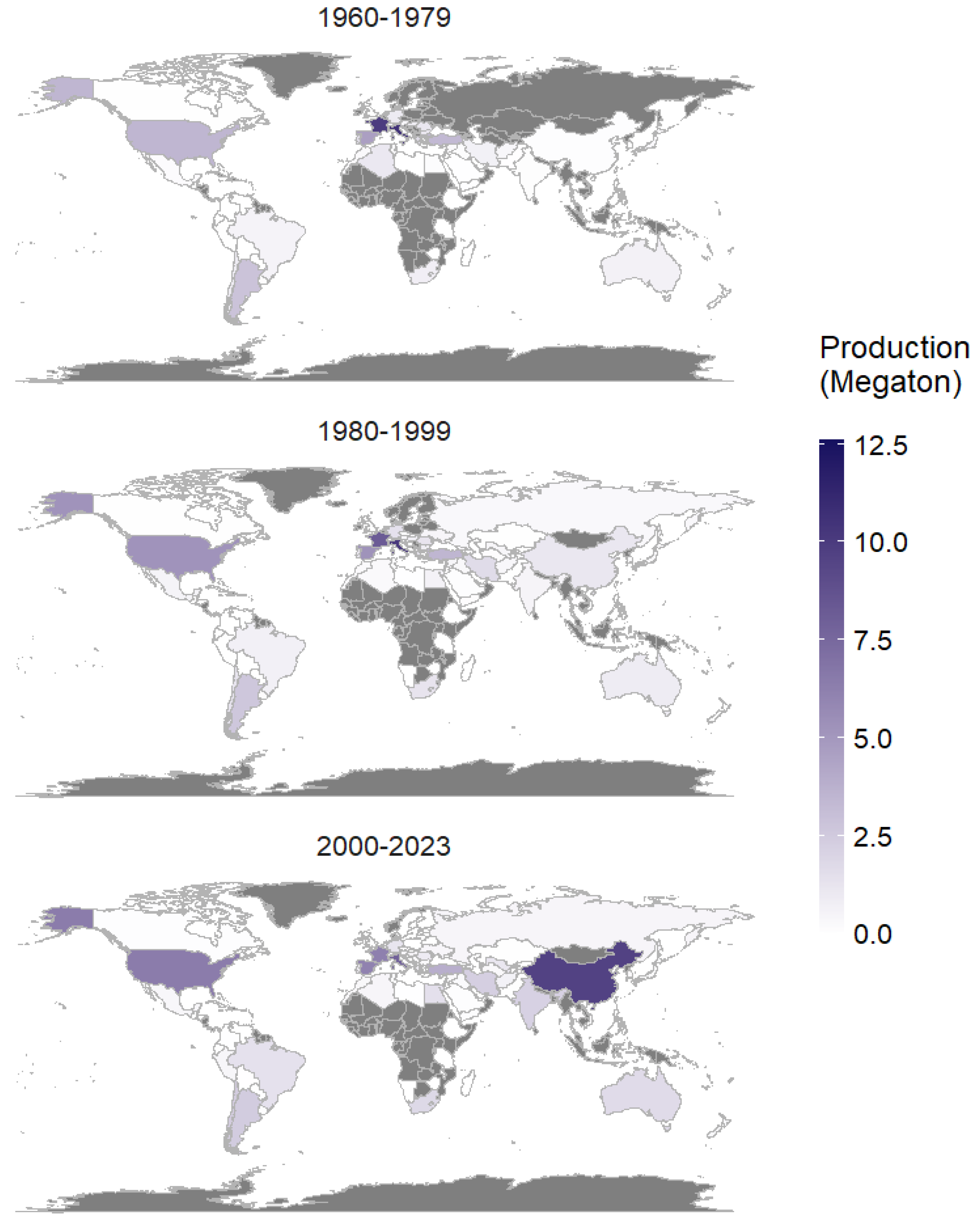
  • Production: this factor represents the annual fresh-grape production for each country, measured in Megaton. A series of world maps with averaged values every two decades can be seen in Appendix A, Figure A1.
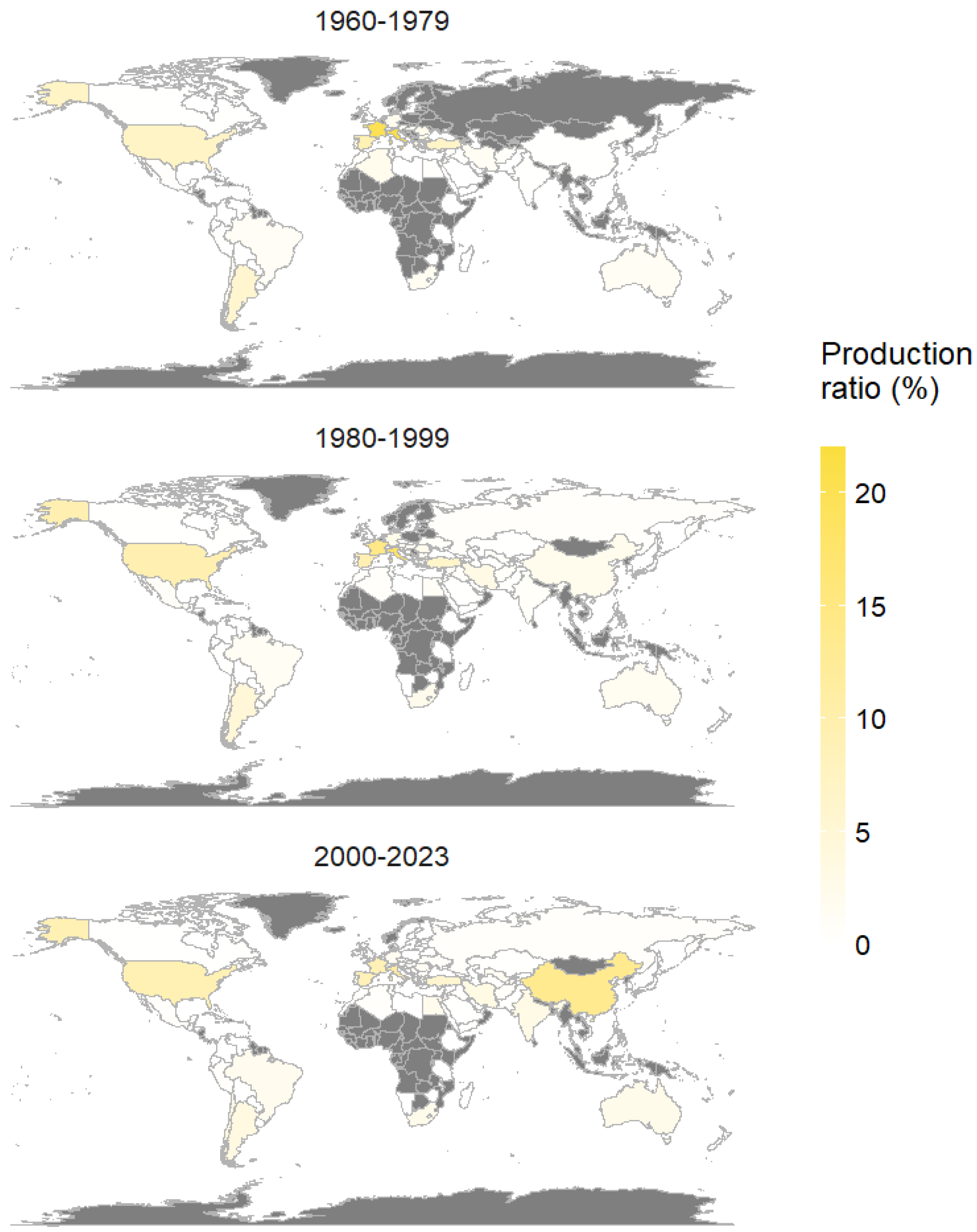
  • Production ratio: all production records were summed to achieve global annual production, then the percentage of each country’s production relative to the global total was calculated for each year. Three world maps of averaged values at 20-year intervals are available in Appendix A, Figure A2.
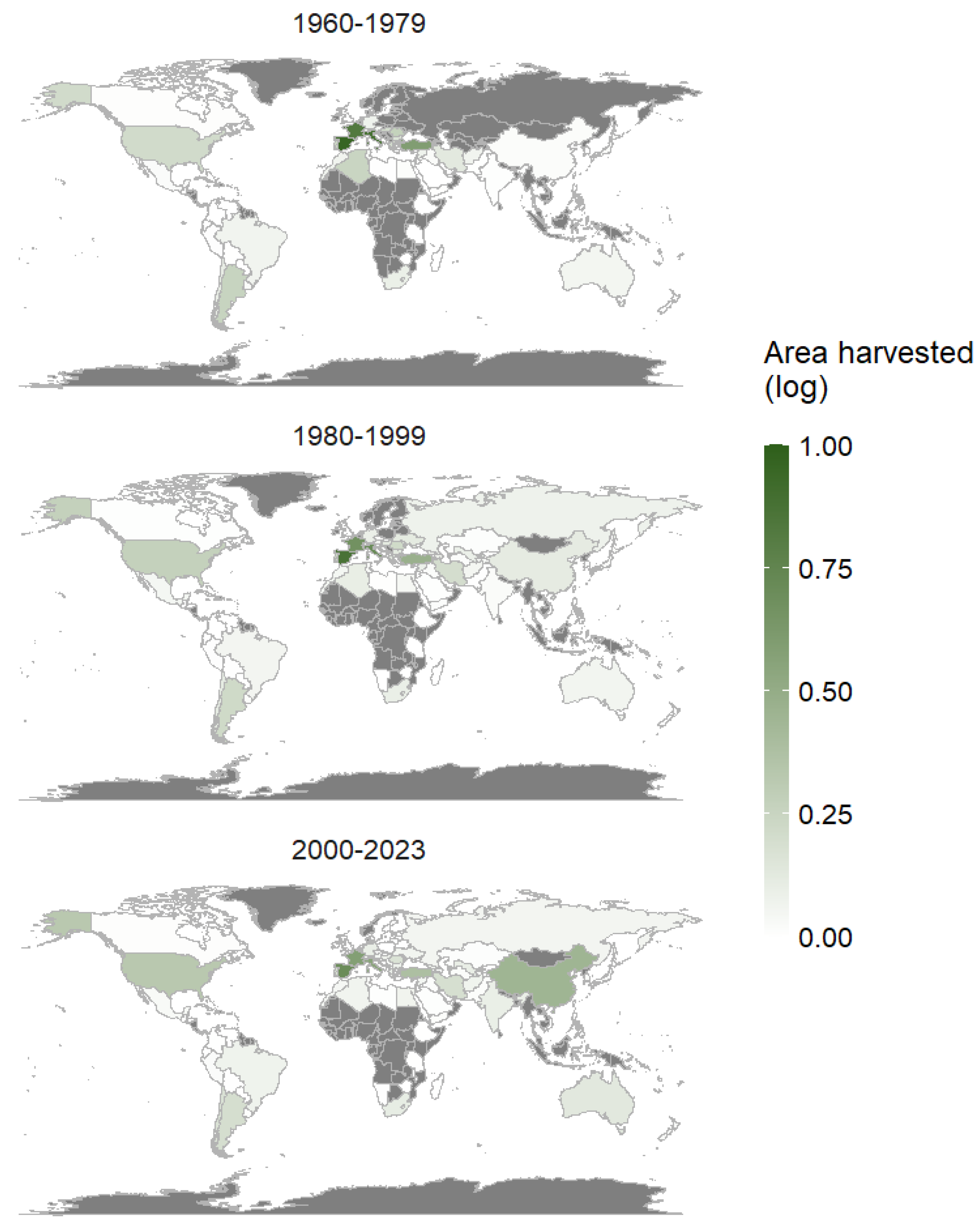
  • Area harvested: This indicates the area coverage of fresh-grape cultivation in each country every year, expressed in million hectares. It signifies the amount of land dedicated to vineyards each year. A series of world maps illustrating the logarithmic representation of averaged values every two decades can be found in Appendix A, Figure A3.
  • Vineyard to cropland ratio: Derived by comparing harvested area to total cropland area (also obtained from the FAO database). This factor represents the proportion of cropland used for annual grape cultivation in each country. Figure A4 in Appendix A presents a series of world maps showing the logarithmic distribution of 20-year average values.
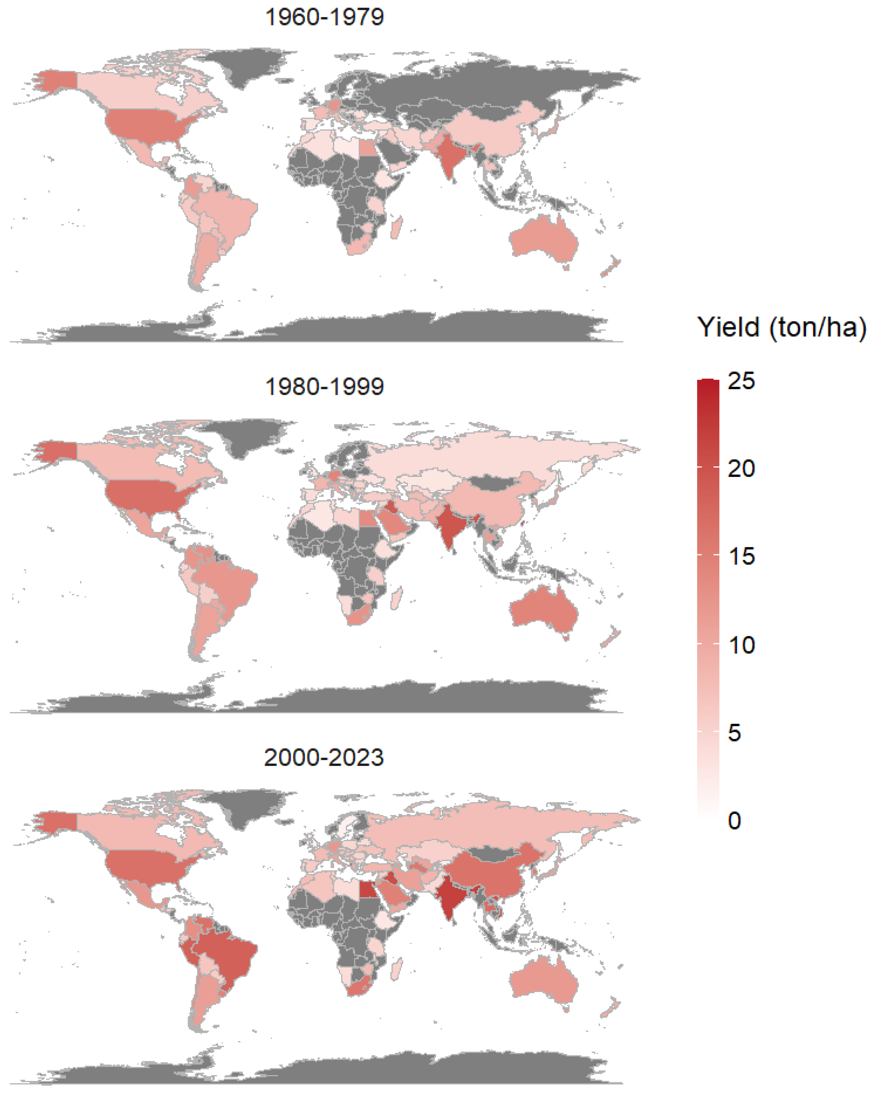
  • Yield: this factor reflects the weight of fresh grapes produced per unit of land, represented in tons per hectare. It indicates the efficiency of vineyard land use, with higher yields signifying better land utilization. The spatial distribution of 20-year average values is shown in the world maps available in Appendix A, Figure A5.
These five factors were constantly available for 84 countries. Figure 1 illustrates the trends of four factors globally. (The production ratio is meaningless at a global scale).
To comprehensively quantify the drivers influencing the area harvested factor, several supporting factors were incorporated into the analysis.
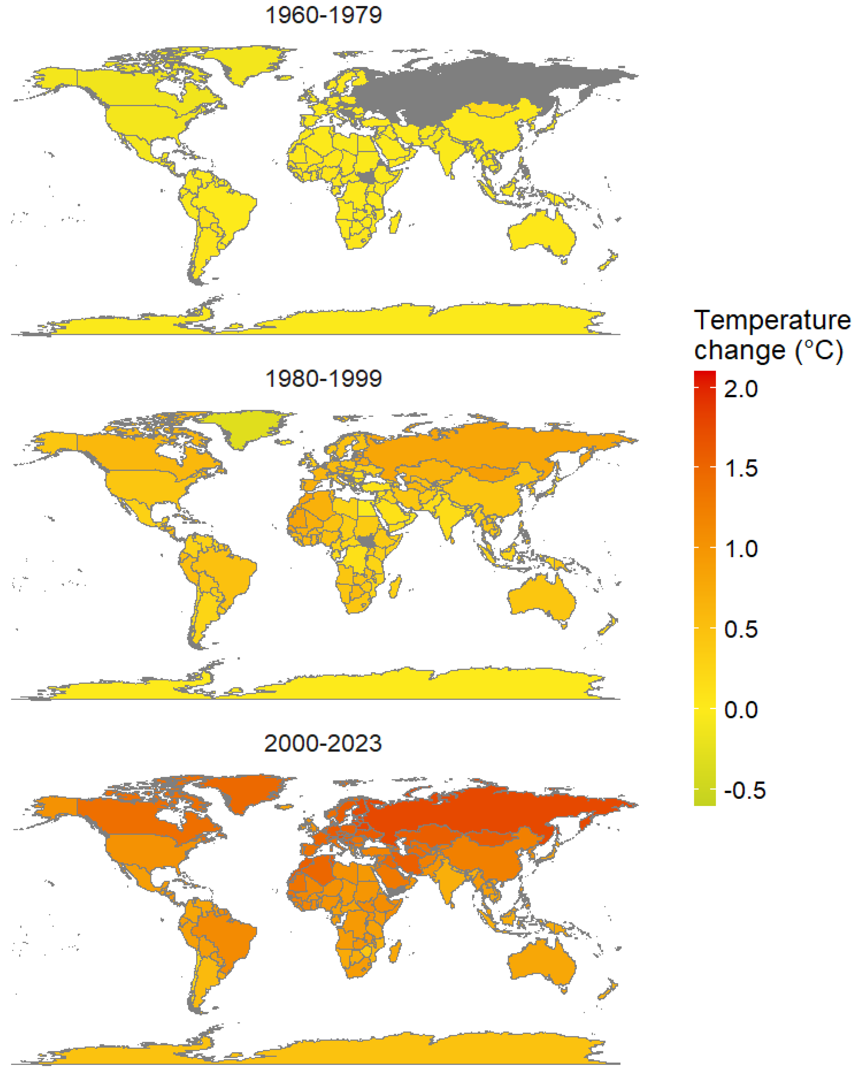
  • Temperature change: This variable represents the deviation in temperature (°C) from a baseline climatology computed for the period 1951–1980. Data were acquired from the FAO database, and the temperature change was calculated relative to this baseline. Mean 20-year maps illustrating these changes are presented in Appendix A, Figure A6.
  • Temperature: Mean temperature values (°C) for each country were obtained from the World Bank Group portal (https://climateknowledgeportal.worldbank.org/download-data, accessed on 8 March 2025). These values were derived from the CMIP6 climate model [40] at a spatial resolution of 0.25 degrees.
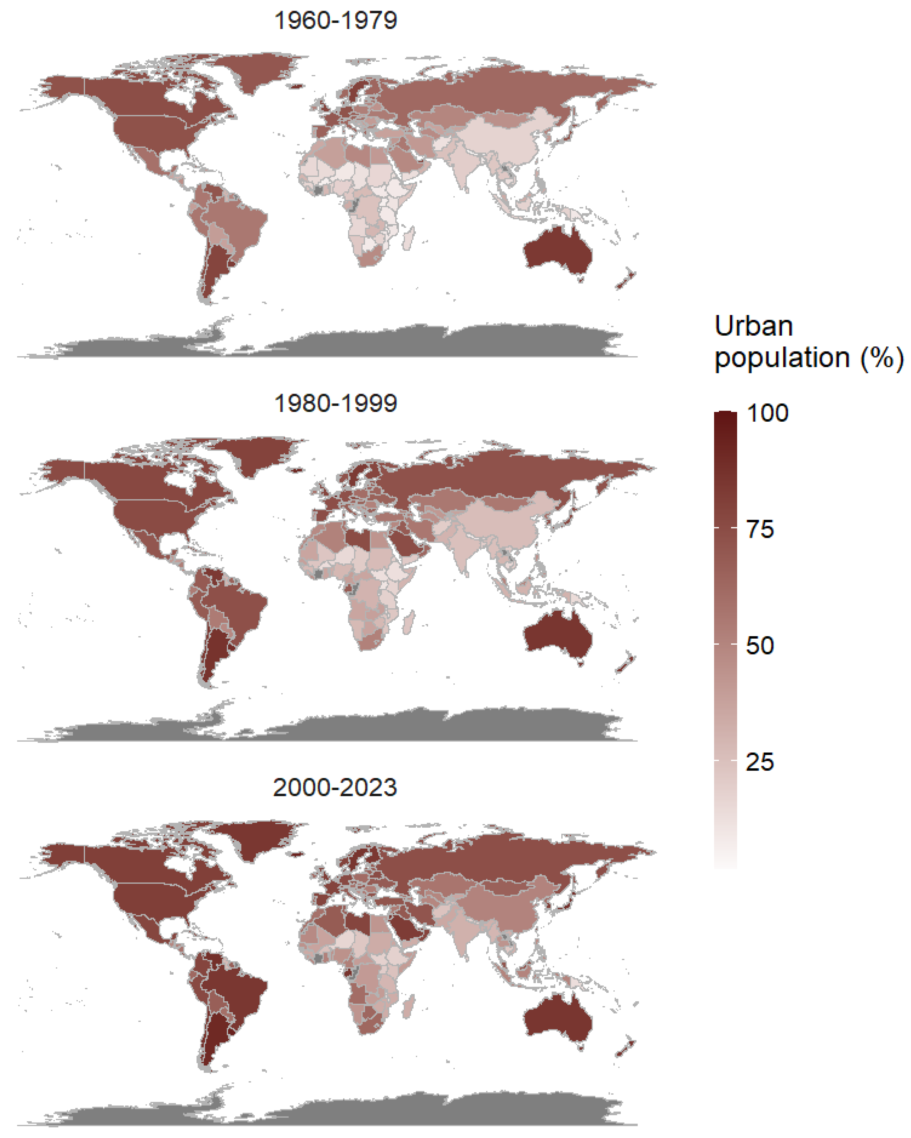
  • Urban population: reflects the annual percentage of each country’s population living in urban areas. Data were acquired from the World Bank Group portal (https://climateknowledgeportal.worldbank.org/download-data, accessed on 8 March 2025). Average 20-year maps for urban population percentages are presented in Appendix A, Figure A7.
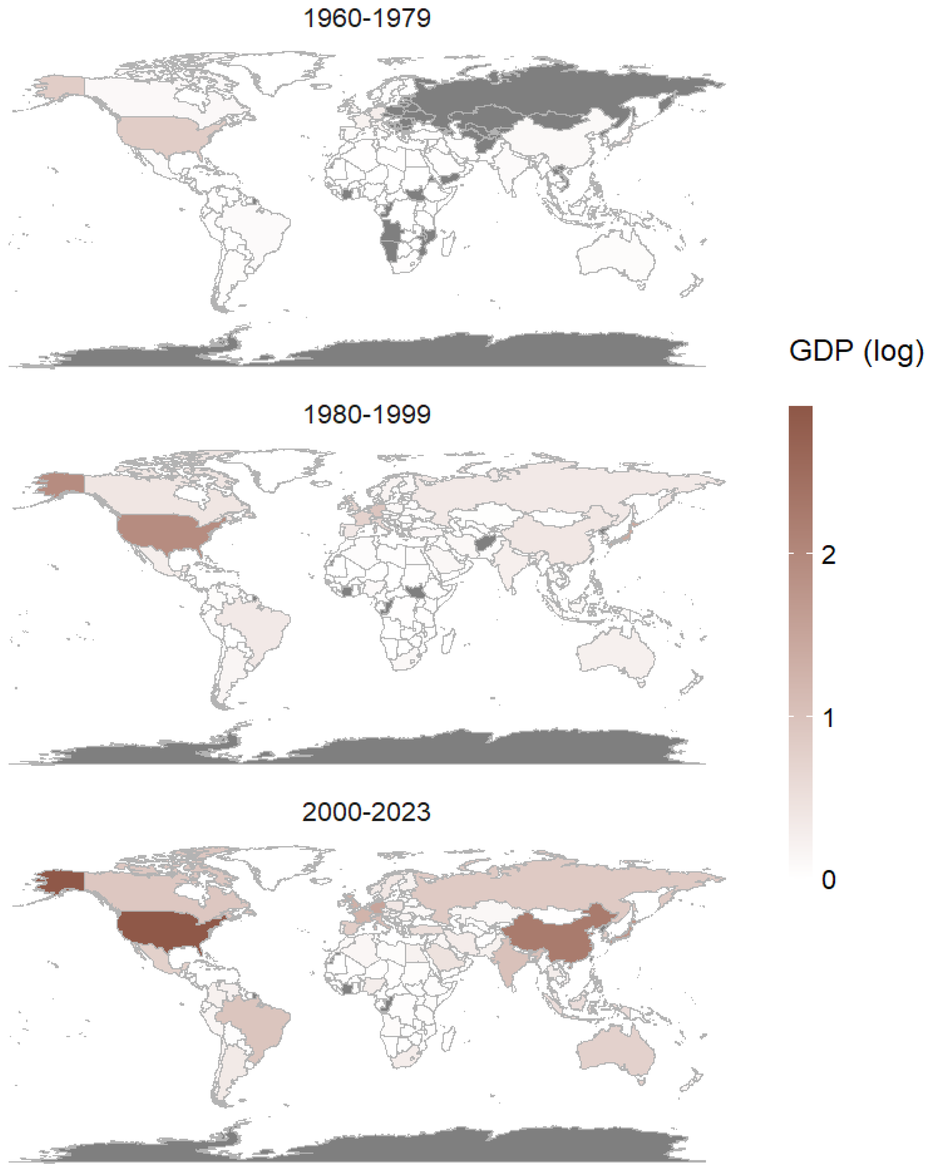
  • Gross Domestic Product (GDP): This represents the total monetary value of all the goods and services produced within a country, serving as an indicator of economic activity and national wealth. The data were acquired from the World Bank Group portal (https://climateknowledgeportal.worldbank.org/download-data, accessed on 6 September 2025) and are given in current US dollars. Three maps averaging every two decades of long-transformed GDP are available in Appendix A, Figure A8.
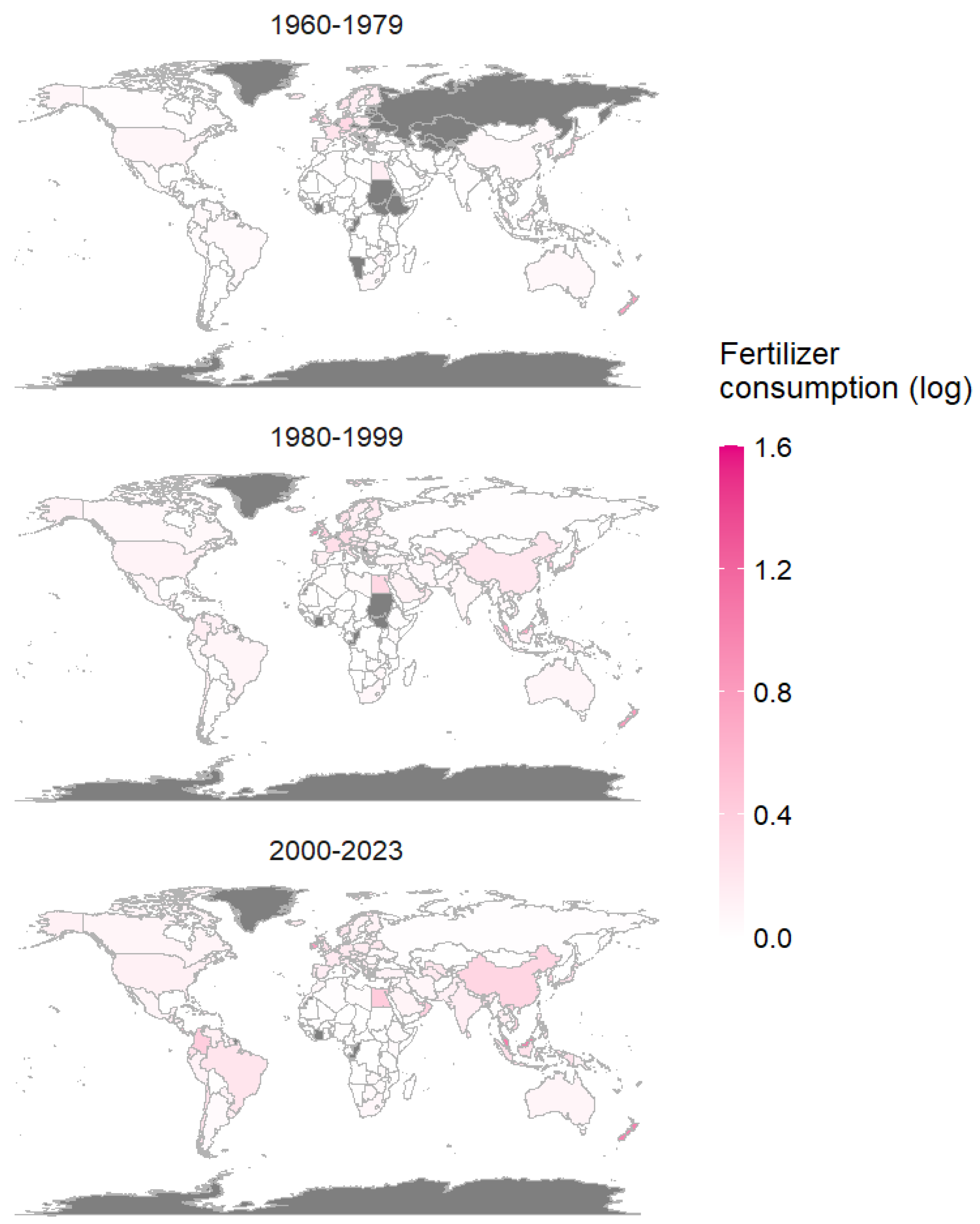
  • Fertilizer consumption: This measures the average intensity of fertilizer use across arable land. It is calculated by dividing the total annual fertilizer consumption by hectares of arable land and is provided in kg/ha per arable land. Fertilizer data at the country scale were acquired from the World Bank Group portal (https://climateknowledgeportal.worldbank.org/download-data, accessed on 6 September 2025). A visual representation of 20-year means is available as maps in Appendix A, Figure A9.

2.2. Long-Term Trends of Area Harvested and Production Factors

The long-term data for each of the five factors (e.g., Production, Production ratio, Area harvested, Vineyard to cropland ratio, and Yield) were used to quantify the temporal trend. Given the large number of time series across multiple countries and variables, and the potential violation of parametric test assumptions, a non-parametric trend test was most appropriate. The temporal trend analysis was conducted using a two-sided Mann–Kendall (MK) trend test, similar to the process described in [3]. The MK trend test is non-parametric and ranks the magnitude and direction of the temporal trend of a time series [41]. The result is a standardized test statistic Z, which follows a normal distribution, and enables the significance of the trend to be determined. The Z-Score enables the direction of the trend (positive, negative, or no change), the significance (p-value that corresponds to the calculated Z-Score), and the magnitude of change to be identified (Z-Score values farther from 0 are associated with a higher magnitude of trend). The MK test is widely used to define temporal trends in market research [3,42], agricultural studies [43,44], environmental studies [45,46], and meteorological research [47]. The MK test was applied using the “trend” package in R version 4.4.3 [48].

2.3. Factors Affecting Area Harvested—Rank and Patterns

To investigate the complex factors influencing the variability in areas harvested across different countries over the 63-year study period, a modeling framework was developed. Specifically, a Random Forest (RF) regression algorithm, a non-parametric machine learning technique, was used to analyze the relationships between area harvested and the following predictor variables: Production, Yield, Temperature, Temperature change, Urban population, Fertilizer consumption, GDP, and Year. This approach enabled us to assess feature importance and characterize the patterns of influence of these predictors on vineyard coverage.
RF is known for its ability to model complex, multivariate relationships. The algorithm is based on constructing an ensemble of decision trees, each trained on a bootstrapped subset of the data. Moreover, at each node split, a random subset of predictors is considered, enhancing model robustness and reducing overfitting. The final prediction is obtained by averaging the predictions of all individual trees [49]. Given its suitability to handle large and diverse datasets, RF has been widely adopted in multi-national studies [50,51].
In this study, the RF model was implemented using the ‘ranger’ package in R [52]. The model was applied using 500 trees, utilizing Gini impurity for node splitting and bootstrap sampling. The minimum node size was 5. The outputs of the model included a ranked list of feature importance and partial dependence plots (PDPs). PDPs were generated to visualize the marginal effect of each predictor on area harvested, while controlling for the influence of other predictors. This means that the PDPs were derived by averaging the model predictions across all observations for each value of the predictor (e.g., holding all other features constant), effectively isolating its impact. The ‘pdp’ package in R version 4.4.3 [53] was used for PDP generation.
To assess model performance and ensure the reliability and validity of the model’s predictions, a validation process was carried out. The dataset was randomly partitioned into training and test sets at a 70:30 ratio. The model was trained on the training set, and the predicted Area harvested values for the test set were subsequently compared to the actual values. Model performance was evaluated using the following statistical metrics:
-
Pearson’s correlation coefficient (r): This statistic measures the strength and direction of the linear association between the model’s predictions and the corresponding actual values. A higher absolute value of r indicates a stronger linear relationship.
-
Paired t-test (t): This test was used to test a statistically significant difference between the mean of the predicted vs. actual values of Area harvested within the test set.
-
Kolmogorov–Smirnov statistic (D): This metric was used to compare the cumulative distribution functions of the predicted and observed Area harvested values in the test set, assessing whether the two distributions are statistically distinct.
-
Mean absolute error (MAE): The average absolute difference between actual and estimated Area harvested values. To facilitate interpretation, the MAE was normalized to the range of the actual values in the test set, expressing the error in percent. The MAE calculation was performed using the ‘Metrics’ library in R [54].

2.4. Temporal Global Variations in Area Harvested and Production Factors

To quantify global variations in Area harvested and Production factors, we first assessed the temporal dependency of each variable. Pearson correlation coefficients were calculated between each of the four global indicators (e.g., Production, Area harvested, Vineyard to cropland ratio, and Yield) against Year, to evaluate the non-stationarity of each time series.
Subsequently, a cross-correlation function (CCF) was applied to investigate temporal association for paired factors. This method quantifies the similarity between two time-dependent series as a function of lag (the time offset between the series). A positive lag indicates that changes in the first variable are followed by changes in the second, whereas a negative lag suggests that the second variable precedes the first. In this way, CCF helps identify whether changes in one variable precede or follow those in the second variable [55]. This approach is particularly useful for detecting delayed or anticipatory relationships and has been applied in various fields, including market research [56,57].
To assess global variability over time, a cross-country coefficient of variation (CV) was calculated annually using available data from all reporting countries. The CV, a measure of dispersion, is defined as the ratio of the standard deviation to the mean, expressed as a percentage. This normalization enables direct comparison of variability across different indicators, regardless of their units. A lower CV reflects lower inter-country heterogeneity and greater consistency in the measured variable, whereas a higher CV indicates greater variability and inconsistency among countries. Constructing a CV-based time series is a commonly used approach for monitoring trends in inequality over time [58,59]. All the global variation analyses were performed in R [60].

3. Results

3.1. Long-Term Trends of Area Harvested and Production Factors

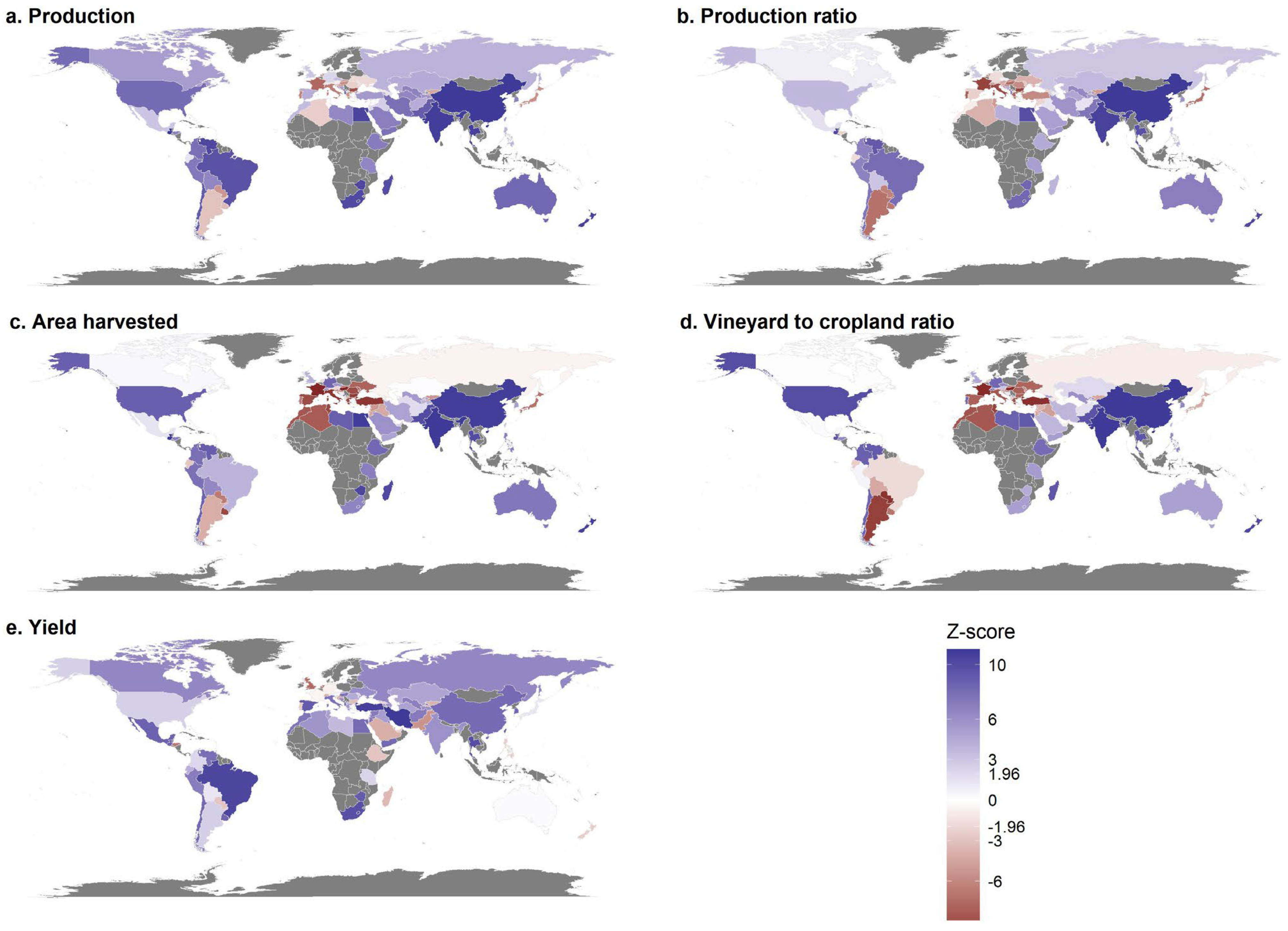
The MK trend test results for the five production and vineyard coverage factors are presented in Figure 2 and reveal significant trends over the 63-year study period. The specific values for each country are available in Appendix B, Table A1. For Production (Figure 2a), our findings show that the majority of countries (50 out of 84) demonstrated a statistically significant positive trend. Interestingly, Guatemala (Z = 11.1), China (Z = 11.08), and India (Z = 10.85) exhibited the strongest positive trends. On the other hand, 20 countries showed negative Production trends, with a high portion of them (12) located in Europe. The strongest negative trends were observed in Bulgaria (Z = −8.87), France (Z = −7.62), and Italy (Z = −6.55). These trends were corroborated by examining the actual Production values. In 2022, China emerged as the leading producer of fresh grapes (15.44 Megaton), followed by Italy (8.43 Megaton), France (6.2 Megaton), and Spain (5.9 Megaton). However, the corresponding Production values in 1963 were significantly lower: China with 0.09 Megaton, Italy with 8.7 Megaton, France with 8.77 Megaton, and Spain with 4.12 Megaton. These data highlight the substantial shifts in global grape production over the study period.
The trends observed for the Production ratio were less pronounced compared to those for absolute Production. Nevertheless, 38 out of the 84 grape-producing countries exhibited statistically significant positive trends (Figure 2b). The most substantial positive trends were recorded for China (Z = 11.09), India (Z = 10.59), and Guatemala (Z = 10.2). However, 33 countries demonstrated significant negative Production ratio trends, with the most extreme declines observed in France (Z = −9.61), Bulgaria (Z = −9.56), and Italy (Z = −9.24). An examination of the actual Production ratio values reveals that in 2022, China accounted for nearly 20% of global fresh grape production, followed by Italy (10.8%), France (9.92%), and Spain (7.54%). In contrast, in 1963, France and Italy were the leading global producers, with 19.9% and 19.7% of global production, respectively. They were followed by Spain (9.31%) and the USA (7.79%). However, China’s Production ratio was only 0.2% of global fresh grape production in 1963.
Analysis of Area harvested trends showed that 36 out of 84 grape-producing countries exhibited statistically significant positive trends (Figure 2c). The strongest increases in vineyard coverage over the 63-year period were observed in India (Z = 11.03), Guatemala (Z = 11.03), Egypt (Z = 10.86), and China (Z = 10.81). Conversely, 31 countries exhibited significant negative trends, with half of these countries located in Europe. The most substantial decreases were recorded in France (Z = −10.94), Hungary (Z = −10.91), Turkey (Z = −10.19), and Italy (Z = −10.17). Our findings can be viewed by the actual Area harvested values, as well. By contrast, in 2022, Spain had the largest vineyard coverage (0.92 million hectares), followed by France (0.76 million hectares), Italy (0.71 million hectares), and China (0.71 million hectares). In contrast, in 1963, European countries accounted for significantly larger vineyard areas, with Italy and Spain each reporting 1.7 million hectares, France with 1.41 million hectares, and China dedicating only 0.01 million hectares for vineyards. The data reveal a significant decline in vineyard coverage across the three key European producers. Over the 63-year study period, France experienced a decrease of 46.10%, Italy a decrease of 58.24%, and Spain a decrease of 45.88%. China, by contrast, experienced an astounding 7000% increase in vineyard area harvested between 1963 and 2022.
Examination of the vineyard to cropland ratio, based on data from 83 countries, revealed that 36 countries exhibited statistically significant positive trends (Figure 2d). These positive trends were most prevalent in Africa (9 countries) and Asia (8 countries). Conversely, 30 countries demonstrated significant negative trends, with a substantial proportion (14 countries, which are 47%) located in Europe. The most pronounced positive trends were observed in India (Z = 10.9), China (Z = 10.84), New Zealand (Z = 10.1), and the USA (Z = 9.68). The strongest negative trends were recorded in France (Z = −10.63), Hungary (Z = −10.57), Turkey (Z = −10.33), Paraguay (Z = −10.23), and Argentina (Z = −9.55). A comparative analysis of the actual Vineyard to cropland ratios indicates that Montenegro currently (as of 2022) dedicates the largest proportion of its cropland to vineyards (19.6%), followed by Georgia (18.2%), Chile (9.77%), and Portugal (9.77%). In contrast, in 1963, Italy had the highest Vineyard to cropland ratio (10.8%), followed by Lebanon (9.26%), Cyprus (9.03%), and Portugal (8.04%).
Yield exhibited the highest frequency of statistically significant positive trends among the analyzed factors (Figure 2e), with 53 out of 84 countries showing a significant increase over the 63-year period. Our findings detected the most substantial positive trends in Iran (Z = 10.32), Turkey (Z = 9.95), and Brazil (Z = 9.6). Conversely, the strongest negative trends were recorded in the United Kingdom (Z = −6.92), the Netherlands (Z = −6.84), and Honduras (Z = −6.34). Analysis of the actual yield values reveals that in 2022, Taiwan had the highest yield (27.5 tons per hectare), followed by Peru (24.39 tons per hectare) and Vietnam (23.97 tons per hectare). However, it seems that in 1963, the leading yield values were reported in Saudi Arabia (30.9 tons per hectare), the Netherlands (22.17 tons per hectare), and India (16 tons per hectare).

3.2. Factors Affecting the Area Harvested—Rank and Patterns

The RF model demonstrated strong predictive performance when evaluated against a randomly sampled test set (Table 1). The normalized MAE was just 0.3%, and the Pearson correlation coefficient was exceptionally high at r = 0.99, indicating high reliability of the model predictions.
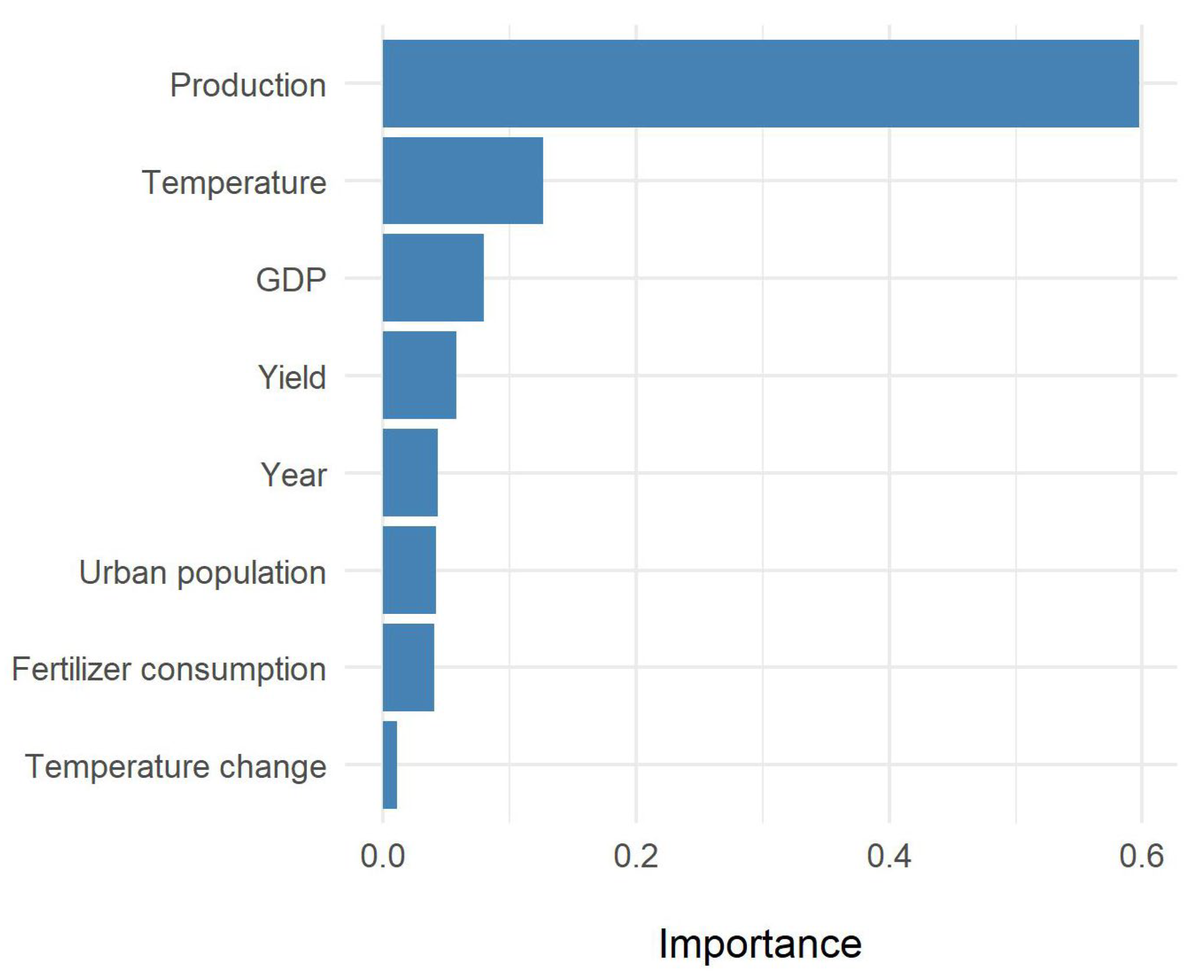
The analysis of feature importance revealed that Production was the dominant driver of Area harvested, accounting for 60% of the model’s predictive power (Figure 3). Other variables had substantially lower influence, including Temperature (13%), GDP (8%), Yield (5.8%), Year, Urban population, and Fertilizer consumption (all 4%), and Temperature change (1%).
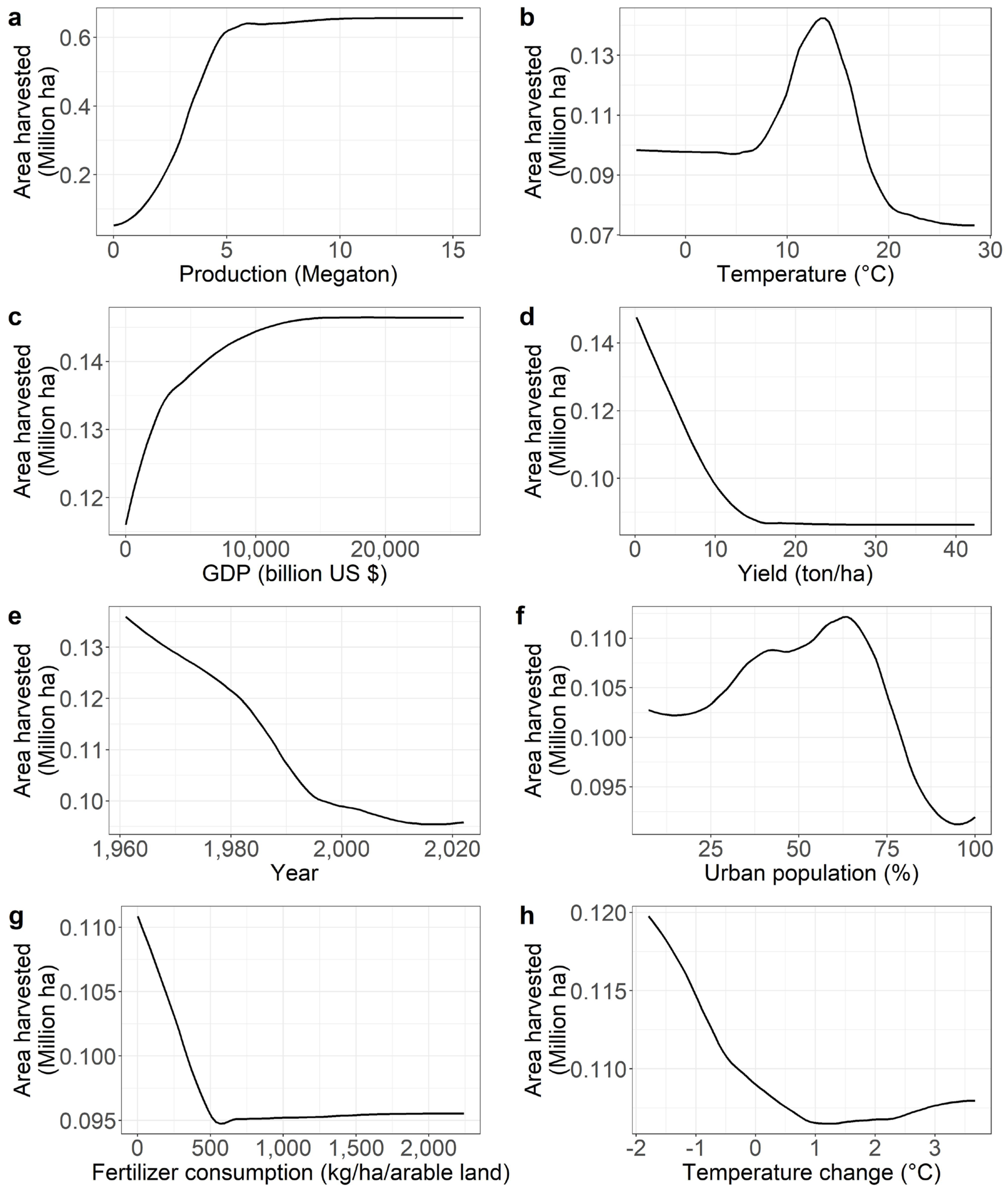
The PDPs illustrate how each feature influences the Area harvested as predicted by the model (Figure 4). Production (Figure 4a) has a strong, though non-linear, positive effect, mainly composed of two linear slopes (up to 5 Megaton and beyond 5 Megaton). Its influence diminishes considerably beyond 5 Megaton, suggesting a saturation point.
An optimal mean annual temperature range for higher values of area harvested was identified between 12 °C and 15 °C (Figure 4b). In regions or periods with average temperatures below 12 °C, the area dedicated to vineyards was found to be lower. Similarly, temperatures above 15 °C were associated with a rapid reduction in vineyard acreage.
Area harvested exhibited a logarithmic relationship with GDP levels (Figure 4c). At lower GDP values, area harvested remained limited, with a sharp increase observed up to approximately 3000 billion US dollars, indicating a strong marginal effect of economic development on vineyard expansion. Beyond this threshold, the rate of increase slowed considerably, and a plateau was reached between 10,000 and 12,000 billion US dollars, suggesting that further economic growth does not substantially drive additional vineyard area expansion. Yield negatively affected the harvested area (Figure 4d). The steepest decline occurred below 15 tons per hectare, beyond which the effect levels off.
We found a declining temporal trend in the Area harvested over the years (Figure 4e), although this decrease became more moderate after 1996. Furthermore, our findings indicate that the urban population (Figure 4f) had a positive influence on the area harvested when below 60%. Above a value of 67%, there was a sharp decline in Area harvested, suggesting that highly urbanized countries tend to allocate less land to vineyard cultivation.
Higher values of Fertilizer consumption were associated with low Area harvested (Figure 4g). At values above 500 kg ha−1, further implementation of fertilizers does not introduce additional Area harvested.
Finally, temperature change seems to have a minimal impact overall (Figure 4h). Negative changes (cooling) were more often associated with larger vineyard areas, whereas no change or a warming of 1 °C was found to be associated with reduced Area harvested. In contrast, increases of 2–3 °C were linked to a slight rise in vineyard allocation.

3.3. Temporal Global Variations in Production and Area Harvested Factors

Correlation analysis between global factors and Year revealed that all variables exhibited significant temporal autocorrelation (Table 2). The Vineyard to cropland ratio showed the weakest association with time. Production and Yield exhibited strong increasing trends over time, while both Area harvested and Vineyard to cropland ratio showed decreasing patterns.
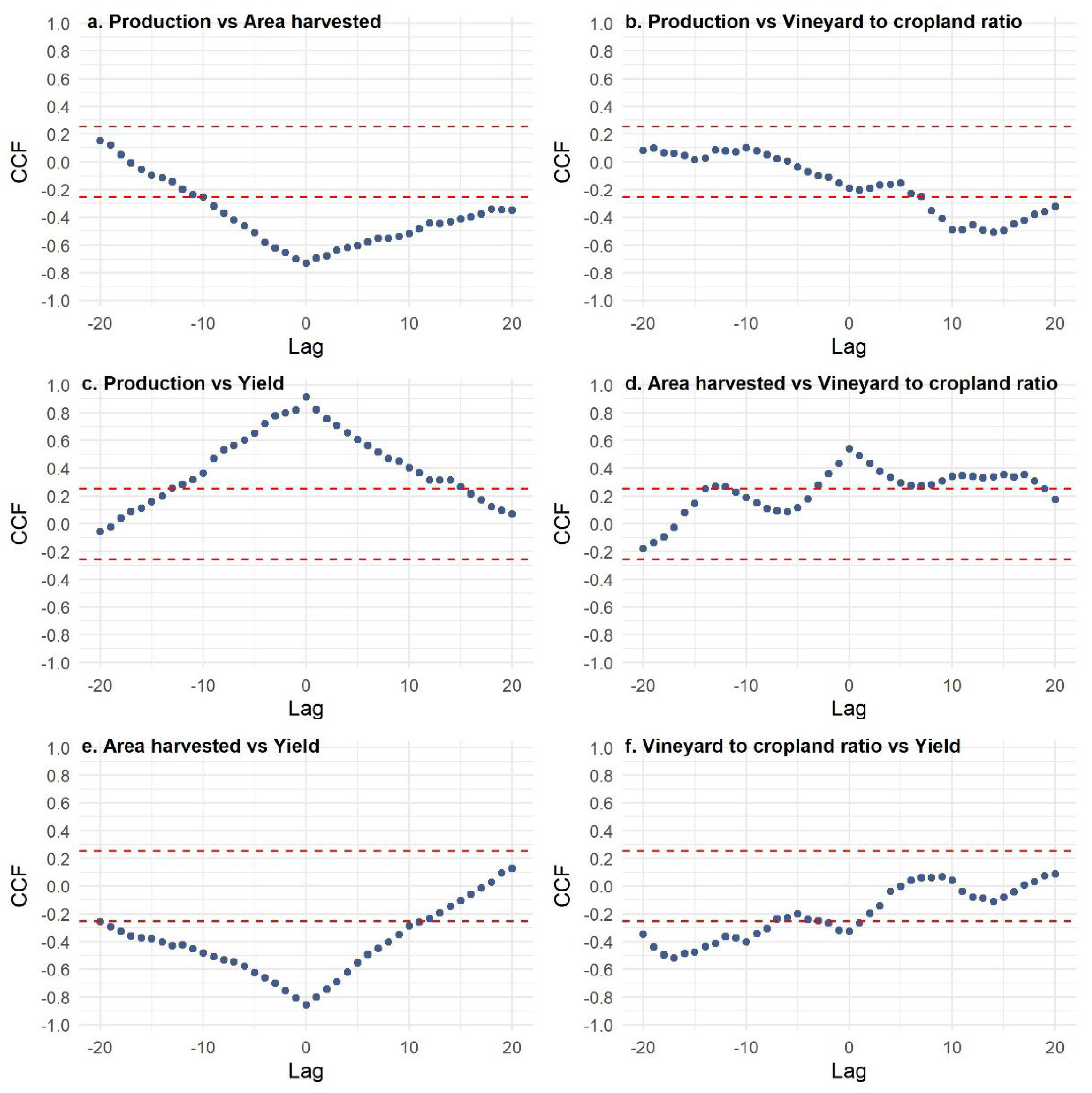
Pairwise analysis of lagged effects showed that most global factors were temporally cross-correlated (Figure 5). The CCF between Production and Area harvested (Figure 5a) showed consistently negative values, indicating that higher production levels were associated with reduced vineyard coverage. At lag 0 (i.e., within the same year), the relationship was the strongest (CCF = –0.73). Negative lags, where Area harvested precedes Production, showed relatively weak correlations, suggesting that it is not a meaningful predictor of future production. In contrast, positive lags—where Production leads Area harvested—revealed slightly stronger associations, indicating that increased production levels tend to result in lower area harvested 1–5 years later. Beyond a 5-year lag, the CCF values dropped below 0.6.
The relationship between Production and the vineyard-to-cropland ratio (Figure 5b) was comparatively weak. The strongest negative correlations emerged when Production led the vineyard to cropland ratio by 10–15 years (CCF values between –0.45 and –0.51), though the overall association remained moderate.
A strong, positive, and symmetrical relationship was observed between Production and Yield (Figure 5c). The correlation peaked at lag 0 (CCF = 0.92), indicating that higher yields are directly associated with higher Production in the same year. Significant correlations persisted at ±5-year lags (CCF > 0.6; CCF < −0.6), suggesting that these variables tend to move together over time.
Area harvested and Vineyard to cropland ratio (Figure 5d) were moderately correlated. The highest association occurred at lag 0 (CCF = 0.54). Positive lags, where the Area harvested leads the vineyard to cropland ratio, showed consistently positive values. This pattern suggests that increases in Area harvested may influence the overall share of cropland dedicated to vineyards in subsequent years.
The relationship between Area harvested and Yield (Figure 5e) was found to be strongly negative at lag 0 (CCF = –0.86), indicating that higher yields were associated with reduced Area harvested. This inverse relationship persisted for up to five years (CCF < –0.6). Conversely, when Area harvested led Yield, the effect was shorter-lived, diminishing after approximately four years.
Finally, we found that associations between the Vineyard to cropland ratio and Yield (Figure 5f) were weak across all lags. However, when vineyard share increased, a subsequent decline in yield was sometimes observed, though these patterns were not consistent or strong across time lags.
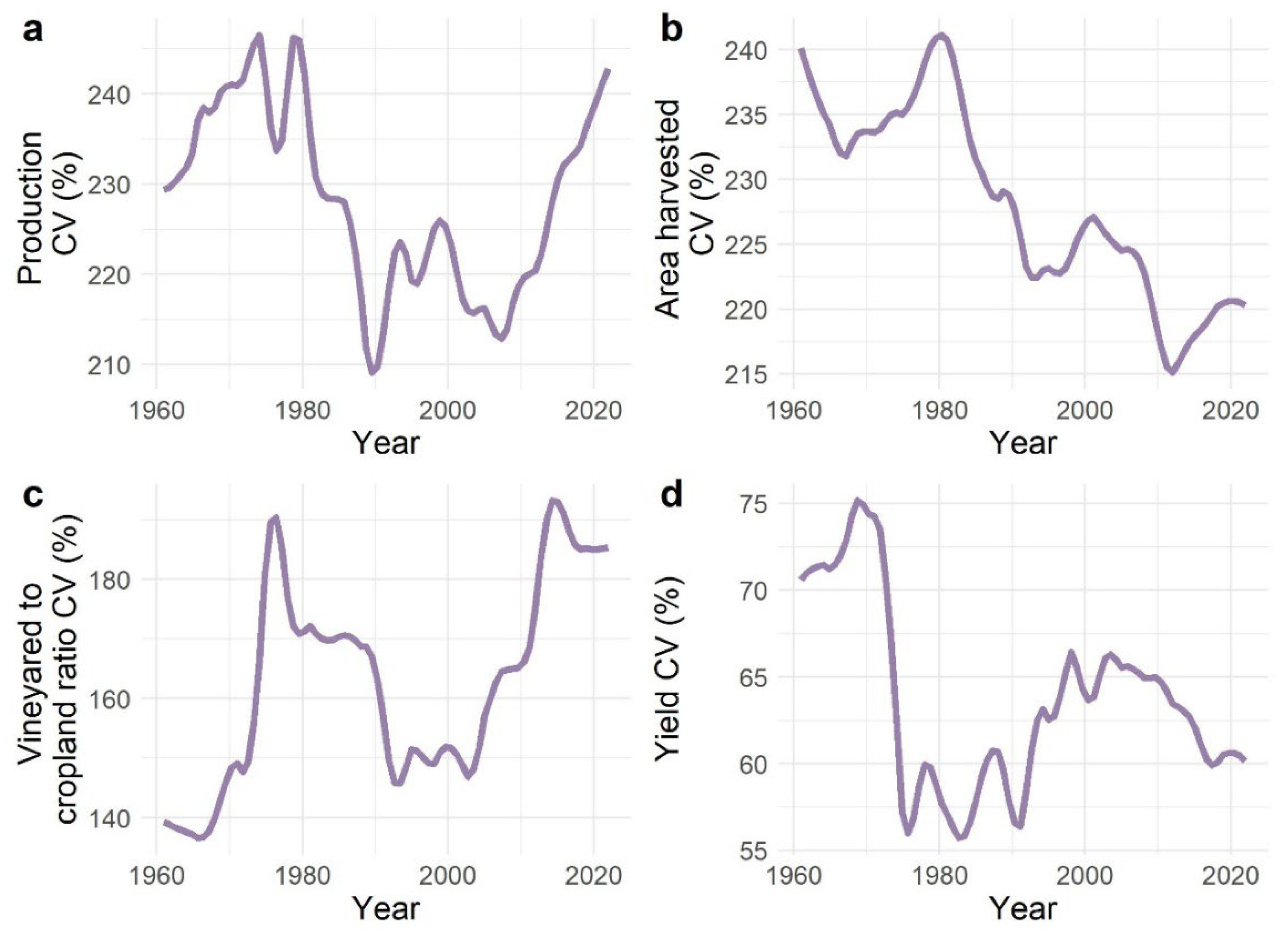
An annual coefficient of variation (CV) was calculated for each of the five key indicators of production and Area harvested, capturing the degree of dissimilarity among global wine-producing countries (Figure 6). The CV range for Production was consistently high throughout the observed period (Figure 6a), ranging between 204% (1991) and peaking at 252% (1979). Noticeably, there were two distinct periods when the CV values reached their lowest levels. First, between 1988 and 1991, and later during 2007–2008. However, beginning in 2009, a steep upward trend in CV values emerged, indicating that production levels across countries are becoming increasingly dissimilar over time. The Production Ratio followed an identical trend, as it is inherently based on the comparison of each country’s production to global totals. Consequently, it was omitted from the figure.
The analysis of CV trends for Area harvested revealed a gradual decrease over the past six decades, though with some intermittent fluctuations (Figure 6b). In 1963, the CV reached 240%, suggesting that while some countries allocated extensive areas to fresh grape cultivation, others devoted very little land to vineyards. In more recent years, however, CV values have stabilized at around 215–220%, indicating a moderate reduction in dissimilarity among countries. Despite this decline, the CV has never decreased below 215%, implying the polarized nature of this factor.
The CV trend for the Vineyard to cropland ratio somewhat resembled that of Production CV over time (Figure 6c). A peak value of 190% was recorded in 1976, followed by a general decline and a period of lower variation between 1992 and 2005. Starting in 2006, a renewed increasing trend was observed, with CV values approaching 200% by 2015.
An examination of the CV trends for Yield (Figure 6d) reveals a gradual decline in between-country variation over time. During the earlier years, particularly between 1967 and 1973, CV values ranged between 70% and 76%, reflecting significant disparities in yield among countries. This was followed by a sharp decline in the mid-1970s. A moderate increase occurred during the mid-1990s, with CV values stabilizing around 65%. However, over the past decade, CV values have decreased once again, indicating a trend toward greater convergence in Yield levels across countries.

4. Discussion

Global shifts in fresh grape production and Area harvested are inherently dynamic processes shaped by temporal trends and geographical forces [2,3]. As large-scale forces such as globalization, climate change, technological progress, urbanization, and shifting land-use patterns intensify, they drive structural changes in both agricultural markets and the landscapes hosting viticulture [37,61]. This discussion explores the long-term trends and patterns of vineyard area and grape production, analyzing the key drivers behind these transformations and their regional variations.
While the data were acquired from a formal database (FAOSTAT), some factors show anomalies during the early 1990s, most likely due to the collapse of the former Soviet Union and a major redistribution of Eastern European countries. These anomalies include sharp shifts in the time series, new countries (some time series only began in the 1990s, as can be seen in Appendix A maps), and the removal of countries. Furthermore, the FAOSTAT data structure does not distinguish between fresh grape types (i.e., table grapes vs. wine grapes).

4.1. Long-Term Reallocation of Vineyard Area

The long-term reallocation of vineyard area reveals pronounced spatial divergence, with established wine-producing regions in Europe undergoing gradual reduction, while emerging economies in Asia and the Americas experience sharp growth. Our analysis underscores substantial declines across major European producers, namely France, Italy, and Spain, expressed by a reduction in production volume, production share, total vineyard area, and the proportion of cropland devoted to viticulture (Figure 2). Contrarily, countries such as China, India, and the USA demonstrate significant positive trajectories across these same metrics, reflecting an ongoing geographic shift in viticultural investment and land use. These findings align with previous patterns found in recent studies [2,3,37,62].
This divergence among countries reflects a complex interplay of policy, environmental, and socio-economic drivers. In Europe, the post-1980s wine surplus crisis led to structural reforms, including vine pull schemes and severe regulations on new plantings, aiming to stabilize the saturated wine market and address the overproduction problem [63,64,65]. Along with the increasing frequency of heatwaves, water scarcity, and declining agroclimatic suitability in southern Europe [61], these pressures have accelerated the reduction in vineyards from traditional regions.
In contrast, it appears that new regions in Eastern Asia are becoming increasingly suitable for growing crops [66,67], and specifically grapes, due to favorable climatic conditions, the adoption of modern viticultural technologies, and fewer regulatory constraints, alongside increasing investments in the table grape market [37]. China is currently the world’s leading fresh-grape producer, accounting for nearly 20% of the global market. This growth is primarily driven by table grape production, which has seen a substantial rise in demand over the past few decades (Appendix A, Figure A1 and Figure A2) [2]. In comparison, the European market remains more focused on wine production, which has experienced a consistent decline in demand [3,6]. India, the second-largest producer globally, also centers its viticultural efforts on table grapes. These efforts make India one of the fastest-growing fresh grape producers [2], largely due to the adoption of diverse modern technologies [68]. This shifting balance between table grape and wine grape production typically delivers higher yields [69], since wine grape cultivation maintains lower yield amounts due to quality constraints, regulations, and cultivation practices. As a result, regions focused on table grapes are expanding production rates rapidly with relatively efficient land use. Traditional wine producers, however, experience stagnation or decline despite maintaining larger vineyard areas. This trend of concentration of production in fewer countries (e.g., China, India) could pose risks to food supply resilience and increase vulnerabilities in the global food system.

4.2. Decoupling of Production from Land Use

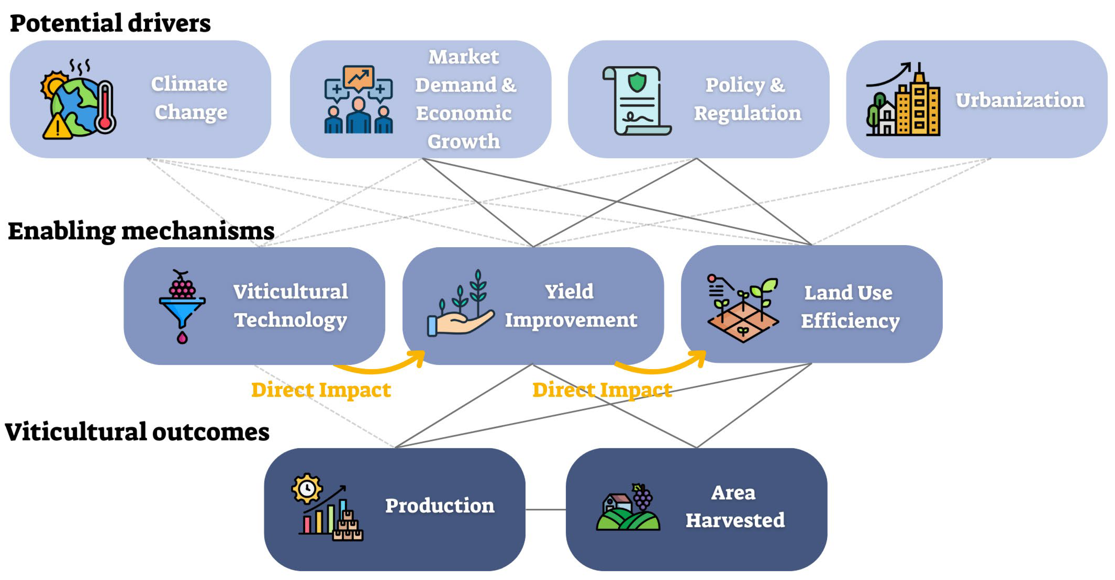
The relationship between grape production and vineyard area is undergoing a major transformation, suggesting a decoupling of production volume from vineyard area requirements, meaning that there is a shift toward producing more with less land. As shown in Figure 7, there are interactions among interconnected factors, which this study attempted to decipher. Our findings using the RF model suggest that Production is the strongest predictor of Area harvested, accounting for 60% of the model’s explanatory power (Figure 3). However, the PDPs revealed that this influence plateaus beyond approximately 5 Megaton (Figure 4a). This indicates a potential land-use ceiling where further production gains do not require proportional increases in cultivated areas. Cross-correlation analysis further supports this trend, as a strong negative association between Production and Area harvested (Figure 5a) at lags of 1–5 years implies that growth in Production is often followed by a contraction in vineyard extent, potentially reflecting optimization or efficiency gains [70].
Furthermore, the CCFs show a near-perfect positive correlation between production and yield at lag 0 (CCF = 0.92) (Figure 5c), suggesting that improvements in yield are a significant driver of increased production, and support the idea that vineyard management practices, rather than land expansion, increasingly drive fresh-grape amounts. This aligns with findings by Tian et al. (2016) [71], who showed that productivity gains, rather than land expansion, have affected grape production in Chinese regions. The work of [24] Cameron et al. (2024) further detailed the role of vineyard management and yield efficiency in modern viticultural systems. In contrast, the strongly negative correlation between yield and area harvested (CCF = –0.86 at lag 0) (Figure 5e) highlights that higher yields are consistently associated with reductions in vineyard area, a trend indicating intensified production systems and reduced land dependence. Together, these patterns imply that land use is becoming increasingly influenced by technological and agronomic improvements in productivity.
In addition to yield dynamics, other factors such as urbanization, economic growth, modern agriculture, and climate also influence vineyard extent. There are known relationships between higher GDP and agricultural land endowment [72], as rising economic growth is a strong driver of crop production dynamics. In this research, higher incomes enable both the utilization of technological intensification in viticulture and a shift in consumer demand toward diversified grape products. The effects of urban encroachment on cropland allocation are highly researched and were widely discussed in the literature [73,74,75,76,77]. Our findings also echo previous studies that analyzed climatic suitability in winegrowing regions and its shifting trends and effects on vineyard distribution [13,15,34,78].
While land allocation has always been shaped by socio-environmental conditions, our findings highlight how some constraints, such as urban pressure, climate suitability, and cropland composition, interact with production efficiency in shaping vineyard area and allocation [79,80]. Land use in viticulture is no longer driven solely by fresh-grape demand but reflects a complex interplay of agronomic potential, environmental constraints, and socio-economic factors. This strengthens a growing recognition in viticultural geography: that the sustainability and efficiency of land use is often more influential to production than simply the extent of land under vineyards.
These findings underline a broader transformation in global viticulture, indicating that production systems are becoming more efficient, increasingly driven by innovations in yield, agronomic management (e.g., fertilization), and strategic land use. Subsequently, grape growers are leveraging improved productivity to sustain or grow crops within a smaller footprint, which is a critical development for future food security, climate resilience, and sustainable land management. However, this decoupling is driven not only by technological intensification and yield-focused innovations in viticulture and land management, but also by structural shifts in market demand, particularly the rapid expansion of the table grape sector in certain regions [37] alongside a reduction in the wine market in others [3]. Table grapes generally produce higher yields than wine grapes, due to differences in cultivation goals, pruning intensity, and harvest practices [81]. As such, countries focused primarily on wine production, including many in Europe, may report consistently lower yields, even when employing advanced technologies [3]. This distinction partly explains the persistent yield gap between traditional wine regions and newer economies that focus on high-output table grape cultivation, such as China and India (Wang et al., 2017) [82].

4.3. Intensification and Technological Gains

The global trend of rising yields across grape-producing countries (Figure 1d) underscores a major transformation in viticultural systems marked by technological intensification and increasingly efficient land use. Our findings reveal that 53 out of 84 countries exhibited statistically significant positive trends in yield over the past six decades (Figure 2, Appendix AFigure A5). These improvements suggest the adoption of advanced agronomic practices and optimized vineyard management in contexts previously constrained by resource limitations or climatic challenges [14].
This intensification is further supported by the strong inverse relationship between yield and area harvested, with CCF of –0.86 at lag 0 (Figure 5e). This suggests that as yields improve, vineyard area tends to contract—reflecting a shift toward “producing more with less”. In essence, higher-yielding systems reduce the need for higher vineyard coverage, enabling countries to meet or exceed production targets while conserving land resources.
Since the 1960s, yield CV has declined steadily, particularly after the mid-1970s, indicating a global convergence in productivity levels (Figure 6d). This trend likely reflects the diffusion of similar technologies and practices across diverse viticultural regions, including precision agriculture, improved irrigation systems, optimized trellising methods, and the widespread use of high-performing cultivars [24].
Beyond productivity, the implications of this intensification are also environmental. As vineyard systems become more technologically efficient, the land-use footprint of viticulture may shrink, thereby reducing the pressure on cropland and natural ecosystems. The trend toward higher yields with reduced spatial demands may support broad goals of sustainability, particularly when coupled with climate-smart and resource-efficient practices [34,83].
Taken together, these results highlight a global shift toward yield-driven efficiency, supported by shared technological trajectories. As more countries converge on similar yield levels and vineyard management strategies, viticulture is increasingly defined not by land expansion but by knowledge, innovation, and adaptability, even as underlying differences between wine and table grape systems continue to shape baseline performance expectations.

4.4. Polarization and Convergence Among Countries

The global CV analysis (Figure 6) highlights an important structural transformation in global viticulture, with a growing polarization in production output alongside a convergence in efficiency and land-use practices during the past 15 years. This dual dynamic suggests that while global fresh-grape production is becoming more concentrated among fewer countries, the methods and productivity levels are becoming more uniform.
Figure 6a shows a sharp increase in Production CV since 2009, reaching levels above 245% by 2022—the highest since the early 1980s. While earlier decades exhibited brief phases of lower variation, the current trajectory is upward, as also shown in [37] Seccia et al. (2015). This pattern points to a widening gap between the largest and smallest producers. The growing concentration is largely driven by the disproportionate rise in Asian producers, especially China, and the stagnation or decline of traditional European producers like France, Italy, and Spain. As a result, the production landscape is becoming increasingly uneven, with a few countries now dominating global supply.
In contrast, the Area harvested CV (Figure 6b) shows a gradual decrease with intermittent fluctuations. This suggests that vineyard land use is becoming more evenly distributed across countries, reflecting global access to more standardized land management practices and vineyard management tools. This assumption is corroborated by the Yield CV (Figure 6d), which follows a similar decreasing trend, with a consistent growth in global Yield (Figure 1d). A sharp drop in Yield CV occurred in the late 1970s and a relatively steady decline since the 1990s, stabilizing around 60%. This convergence suggests a widespread diffusion of improved viticultural technologies and agronomic knowledge [22], helping countries achieve comparable productivity levels regardless of geography or scale. This means that Yield values are globally increasing, and at the same time, Yield values are becoming more similar among countries.
The Vineyard to cropland ratio CV (Figure 6c) presents a more complex and unstable pattern. After peaking around 1980 and stabilizing during the 1990s and early 2000s, it increased again in the last decade and a half. This indicates divergent regional strategies in allocating cropland to vineyards. While some regions, such as parts of Asia, eastern parts of Africa and North and Central America, have increased their vineyard shares relative to cropland (Figure 2), others—particularly in Europe—have reduced vineyard land, possibly due to urbanization, policy changes, climate change, shifting economic priorities, or a mix of these drivers.
There is a growing demand for production to ensure food security in response to rapid population growth. However, discrepancies in cropping potential, regulations, and advanced technology across regions lead to cropland pressure in some areas and food insecurity in others [84,85]. There are substantial inequalities within the global food system, which call for strategies that support the increase in production without the proportional increases in cropland area [84]. Our findings show that the viticultural sector complies well with these current needs, as production keeps increasing, whereas the Area harvested is decreasing (Figure 1a,b). However, the centralized trends in recent years, in which five countries produce over 50% of the global fresh grapes annually, promote food insecurity among less-productive countries [86].

5. Summary and Conclusions

This study provides a comprehensive, data-driven analysis of long-term global trends in vineyard coverage and fresh grape production from 1961 to 2023, integrating data from all grape-producing countries and applying advanced statistical and machine learning methods. Our findings reveal that global grape production has increased despite reductions in vineyard area, suggesting a decoupling that may be linked to technological innovation and higher yields, particularly in table grape systems. The findings show how viticultural activity is shifting from traditional European wine regions toward emerging economies like Eastern Asia, likely reflecting changing market demands and regulatory contexts. While production appears increasingly concentrated among a few countries, yield and efficiency trends show signs of global convergence, possibly due to wider adoption of precision agriculture technologies. Finally, vineyard area allocation is associated with multiple factors, highlighting the complex interplay of environmental, economic, and demographic forces shaping global viticulture.
As global demand for grape products, particularly for table grapes in emerging markets, continues to grow, these patterns carry important implications for agricultural sustainability, food security, and climate adaptation. Our results point to potential for the viticulture sector to increase production while limiting land expansion, which is a crucial characteristic in the face of continuous population growth, escalating environmental pressures, and finite agricultural land. However, the observed centralization of grape production among a small group of countries may pose risks for food system resilience and equity. Policy and technological investments should aim to support more equitable access to innovations, as well as adaptation strategies to climate change, particularly in lower-income or climate-vulnerable regions. Further research should explore and validate the underlying drivers of these trends. Disaggregating wine and table grape systems, integrating varietal-level data, and including additional global-scale drivers such as trade intensity, rural labor availability, other climatic factors (e.g., precipitation, drought indices, evapotranspiration), and consumption preferences may assist in further deepening our understanding of the factors shaping sustainable viticultural practices.

Author Contributions

Conceptualization, N.O.-L. and Y.N.; methodology, N.O.-L.; software, N.O.-L.; validation, N.O.-L. and Y.N.; formal analysis, N.O.-L.; investigation, N.O.-L. and Y.N.; resources, Y.N.; data curation, N.O.-L.; writing—original draft preparation, N.O.-L.; writing—review and editing, Y.N.; visualization, N.O.-L.; supervision, Y.N.; project administration, Y.N.; funding acquisition, Y.N. All authors have read and agreed to the published version of the manuscript.

Funding

This work was funded by the Israeli Ministry of Science and Technology via their support through the Eastern R&D Center.

Data Availability Statement

The dataset for this study is freely available from the FAOSTAT database (Food and Agriculture Organization, https://www.fao.org/faostat, accessed 8 March 2025). Global temperature data is freely available from the World Bank Group portal (https://climateknowledgeportal.worldbank.org/download-data, accessed 8 March 2025).

Acknowledgments

We extend our sincere gratitude to Jacob Levi for his invaluable support and expert guidance on the graphical aspects of this work. We also acknowledge the FAOSTAT database as the source of the data used in this study, and we greatly appreciate their efforts and dedication in making these data freely accessible to the research community. During the preparation of this work, the authors used generative AI-based language models (ChatGPT version GPT-4 and GPT-5) to assist with language editing, grammar correction, and phrasing refinement. Furthermore, AI tools were utilized to assist with code preparation for figure generation in R, using the ggplot2 library. No AI tools were used to generate scientific content, perform data analysis, produce figures or tables, or contribute to the interpretation of results. All scientific insights, data processing, and conclusions presented in this article are the sole work of the authors.

Conflicts of Interest

The authors declare no conflicts of interest. The funders had no role in the design of the study; in the collection, analyses, or interpretation of data; in the writing of the manuscript; or in the decision to publish the results.

Abbreviations

The following abbreviations are used in this manuscript:
FAOFood and Agriculture Organization
MKMann–Kendall
RFRandom Forest
PDPPartial Dependence Plots
MAEMean Absolute Error
CCFCross-Correlation Function
CVCoefficient of Variation

Appendix A

The following maps show how various factors have changed over time, grouped into three maps, averaging 2 decades: 1961–1979, 1980–1999, 2000–2023. Each map represents the average value of each factor for each country within the three periods. In cases where the differences in values were too large to visualize clearly, a log transformation (base 10) was applied to enhance comparability. Countries in grey lack data on the specific factor and timeframe.
Figure A1. A series of maps showing mean fresh grape production every two decades from 1960 to 2023.
Agriculture 15 01976 g0a1
Figure A2. A series of maps showing the mean fresh grape production ratio (percentage of global production) every two decades from 1960 to 2023.
Agriculture 15 01976 g0a2
Figure A3. A series of maps showing the mean area harvested (area designated to vineyard) every two decades from 1960 to 2023 after log-transformation.
Agriculture 15 01976 g0a3
Figure A4. A series of maps showing the mean vineyard to cropland ratio (percentage of cropland dedicated to vineyards) every two decades from 1960 to 2023, after log-transformation.
Agriculture 15 01976 g0a4
Figure A5. A series of maps showing the mean yield every two decades from 1960 to 2023.
Agriculture 15 01976 g0a5
Figure A6. A series of maps showing the mean temperature change (with respect to a baseline climatology, corresponding to the period 1951–1980) for every two-decades from 1960 to 2023.
Agriculture 15 01976 g0a6
Figure A7. A series of maps showing the mean urban population every two decades from 1960 to 2023.
Agriculture 15 01976 g0a7
Figure A8. A series of maps showing the mean GDP every two decades from 1960 to 2023 after log-transformation.
Agriculture 15 01976 g0a8
Figure A9. A series of maps showing the mean fertilizer consumption every two decades from 1960 to 2023 after log-transformation.
Agriculture 15 01976 g0a9

Appendix B

A list of Mann–Kendall trend test results in Z-scores for the factors: total production, production ratio (percentage of global production), area harvested (area designated to vineyards), vineyard to cropland ratio (percentage of cropland dedicated to vineyards), and yield. Z-scores higher than 1.96 and lower than −1.96 mark a significant change (α = 0.05). These values are visualized in the maps provided in Figure 2.
Table A1. Z-Score values following a Mann–Kendall significance test for the period between 1961 and 2023, complementary to Figure 2. The analyzed factors are Area harvested, Production, Production ratio, Vineyard to cropland ratio, and Yield, available for all grape-producing countries.
CountryArea HarvestedProductionProduction RatioVineyard to Cropland RatioYield
Afghanistan1.874.371.491.556.68
Albania−1.498.297.01−2.57.37
Algeria−8.27−2.43−3.82−8.365.25
Argentina−3.96−2.98−7.16−9.552.38
Armenia−0.924.042.61−1.025.11
Australia7.328.346.954.920.2
Austria−1.84−0.85−4.253.160.46
Azerbaijan−0.311.540.89−1.095.46
Bahrain5.138.262.338.54−2.06
Bolivia6.356.553.06−4.231.23
Bosnia and Herzegovina1.095.274.391.095.82
Brazil3.939.617.97−1.779.62
Bulgaria−9.89−8.87−9.56−7.75−3.01
Canada0.45.290.870.116.01
Chile8.469.067.498.427.62
China10.8111.0811.0910.857.59
Colombia7.817.916.718.581.93
Croatia−5.43−5.3−5.95−5.23−4.23
Cyprus−9.75−6.39−7.15−5.3−0.56
Czech Republic5.613.50.826.42−0.24
Ecuador−2.771.36−1.73−2.423.87
Egypt10.8610.449.769.067.5
Ethiopia8.287.134.487.95−2.64
France−10.94−7.62−9.61−10.63−0.51
Georgia−0.79−1.15−2.294.76−1.88
Germany8.432.21−1.748.24−0.64
Greece−9.31−5.41−7.83−8.655.09
Guatemala11.0311.1110.29.267.91
Honduras6.796.79−2.216.27−6.34
Hungary−10.91−5.58−7.41−10.577.05
India11.0310.8510.5910.95.49
Iran4.857.865.743.7410.32
Iraq−4.22.531.4−4.684.84
Israel−1.420.88−2.7−1.72.05
Italy−10.17−6.55−9.24−8.397.16
Japan−7.02−5.56−7.12−4.021.22
Jordan−4.442.050.26−4.356.94
Kazakhstan0.184.463.621.944.43
Kuwait0.886.255.86−0.938.08
Kyrgyzstan−5.24−4.36−4.98−4.39−3.49
Lebanon−5.63−1.2−3.53−4.957.3
Libya8.766.44.228.53.39
Madagascar10.149.933.919.18−3.27
Malta−0.87−0.78−3.681.91−1
Mexico1.43.041.60.248.02
Moldova−7.22−1.38−2.94−5.542.19
Morocco−8.433.54−0.89−8.556.97
Netherlands−2.11−5.28−5.79−3.18−6.85
New Zealand10.5910.5210.210.11−2.27
North Macedonia−4.092.12−1.833.163.81
Pakistan9.968.987.499.38−4.98
Paraguay−6.54−5.25−6.35−10.23−2.66
Peru7.737.346.70.566.56
Philippines6.8543.66.18−2.23
Portugal−6.61−6.14−8.078.16−2.29
Qatar0.33−0.89−1.1−1.04−4.25
Reunion0.75−2.56−3.885.68−3.35
Romania−9.09−2.35−5.8−7.914.18
Russia−0.584.013−0.876.02
Saudi Arabia5.876.925.113.79−3.69
Slovakia−6.66−4.83−5.88−6.533.81
Slovenia−6.86−3.32−5.53−4.96−1.67
South Africa6.610.188.295.089.05
South Korea5.146.85.776.57.72
Spain−9.114.32−2.29−7.918.43
Switzerland6.04−1.22−5.157.05−3.96
Syria−5.110.38−2.04−3.636.69
Taiwan2.895.563.973.717.88
Tajikistan4.065.955.530.855.69
Tanzania6.926.535.185.222.08
Thailand9.9110.699.669.219.13
Tunisia−9.4−0.26−4.9−9.434.79
Turkey−10.195.46−5.84−10.339.95
Turkmenistan1.856.54.69−0.074.56
Ukraine−7.83−1.93−3.84−7.685.63
United Arab Emirates2.430.11−0.33−0.87−2.23
United Kingdom4.153.012.864.65−6.92
Uruguay−9.26−3.28−6.76−6.797.88
USA8.738.153.729.682.3
Uzbekistan5.346.76.375.816.37
Venezuela8.8510.319.188.977.33
Yemen4.847.675.555.097.64
Zimbabwe10.2810.268.424.328.42

References

  1. Rafique, R.; Ahmad, T.; Kalsoom, T.; Khan, M.A.; Ahmed, M. Climatic Challenge for Global Viticulture and Adaptation Strategies. In Global Agricultural Production: Resilience to Climate Change; Springer: Cham, Switzerland, 2022; pp. 611–634. [Google Scholar] [CrossRef]
  2. Alston, J.M.; Sambucci, O. Grapes in the World Economy. In The Grape Genome; Springer: Cham, Switzerland, 2019; pp. 1–24. [Google Scholar] [CrossRef]
  3. Ohana-Levi, N.; Netzer, Y. Long-Term Trends of Global Wine Market. Agriculture 2023, 13, 224. [Google Scholar] [CrossRef]
  4. Pisciotta, A.; Barone, E.; Di Lorenzo, R. Table-Grape Cultivation in Soil-Less Systems: A Review. Horticulturae 2022, 8, 553. [Google Scholar] [CrossRef]
  5. Fraga, H.; Freitas, T.R.; Fonseca, A.; Fernandes, A.; Santos, J.A. Climate change implications on the viticulture geography. Adv. Bot. Res. 2024, 110, 27–69. [Google Scholar] [CrossRef]
  6. Banks, G.; Overton, J. Old World, New World, Third World? Reconceptualising the Worlds of Wine. J. Wine Res. 2010, 21, 57–75. [Google Scholar] [CrossRef]
  7. Mariani, A.; Pomarici, E.; Boatto, V. The international wine trade: Recent trends and critical issues. Wine Econ. Policy 2012, 1, 24–40. [Google Scholar] [CrossRef]
  8. Mariani, A.; Pomarici, E. Barriers to Wine trade. In The Palgrave Handbook of Wine Industry Economics; Palgrave Macmillan: London, UK, 2019; pp. 291–315. [Google Scholar] [CrossRef]
  9. Ruiz del Castillo, M.L. Table grapes: Health implications and approaches to improve the quality during the cultivation. Adv. Bot. Res. 2025, 113, 179–210. [Google Scholar] [CrossRef]
  10. Chang, J.; Jiang, H. Spatio-Temporal Differentiations and Influence Factors in China’s Grain Supply Chain Resilience. Sustainability 2023, 15, 8074. [Google Scholar] [CrossRef]
  11. Han, Y.; Goetz, S.J.; Schmidt, C. Visualizing Spatial Economic Supply Chains to Enhance Sustainability and Resilience. Sustainability 2021, 13, 1512. [Google Scholar] [CrossRef]
  12. Sweeney, S.; Steigerwald, D.G.; Davenport, F.; Eakin, H. Mexican maize production: Evolving organizational and spatial structures since 1980. Appl. Geogr. 2013, 39, 78–92. [Google Scholar] [CrossRef]
  13. van Leeuwen, C.; Sgubin, G.; Bois, B.; Ollat, N.; Swingedouw, D.; Zito, S.; Gambetta, G.A. Climate change impacts and adaptations of wine production. Nat. Rev. Earth Environ. 2024, 5, 258–275. [Google Scholar] [CrossRef]
  14. Naulleau, A.; Gary, C.; Prévot, L.; Hossard, L. Evaluating Strategies for Adaptation to Climate Change in Grapevine Production–A Systematic Review. Front. Plant Sci. 2021, 11, 607859. [Google Scholar] [CrossRef] [PubMed]
  15. van Leeuwen, C.; Destrac-Irvine, A.; Dubernet, M.; Duchêne, E.; Gowdy, M.; Marguerit, E.; Pieri, P.; Parker, A.; de Rességuier, L.; Ollat, N. An Update on the Impact of Climate Change in Viticulture and Potential Adaptations. Agronomy 2019, 9, 514. [Google Scholar] [CrossRef]
  16. Sgubin, G.; Swingedouw, D.; Mignot, J.; Gambetta, G.A.; Bois, B.; Loukos, H.; Noël, T.; Pieri, P.; de Cortázar-Atauri, I.G.; Ollat, N.; et al. Non-linear loss of suitable wine regions over Europe in response to increasing global warming. Glob. Change Biol. 2023, 29, 808–826. [Google Scholar] [CrossRef]
  17. Wang, S.; Deng, O.; Reis, S.; Zhu, Y.-G.; Xu, J.; Gu, B. Global urbanization benefits food security and nature restoration. Resour. Conserv. Recycl. 2025, 216, 108174. [Google Scholar] [CrossRef]
  18. Ohana-Levi, N.; Givati, A.; Alfasi, N.; Peeters, A.; Karnieli, A. Predicting the effects of urbanization on runoff after frequent rainfall events. J. Land Use Sci. 2017, 13, 81–101. [Google Scholar] [CrossRef]
  19. Jackson, L.; Haden, V.R.; Wheeler, S.M.; Hollander, A.D.; Perlman, J.; O’Green, T.; Mehta, V.K.; Clark, V.; Williams, J. Vulnerability and Adaptation to Climate Change in California Agriculture. Davis, California. 2012. Available online: https://escholarship.org/uc/item/1bs0h6pk (accessed on 22 April 2025).
  20. Di Chiara, V.; Battistella, A.; Boatto, V.; Furlan, S.; Giavi, L.; Liggieri, S.; Paiola, A.; Pomarici, E.; Stefanucci, S. Collaborative Approach for Achieving Ambitious Sustainability Goals: The Prosecco Sustainability Project. Sustainability 2024, 16, 583. [Google Scholar] [CrossRef]
  21. Sánchez-Hernández, J.L.; Aparicio-Amador, J.; Alonso-Santos, J.L. The shift between worlds of production as an innovative process in the wine industry in Castile and Leon (Spain). Geoforum 2010, 41, 469–478. [Google Scholar] [CrossRef]
  22. Ferro, M.V.; Catania, P. Technologies and Innovative Methods for Precision Viticulture: A Comprehensive Review. Horticulturae 2023, 9, 399. [Google Scholar] [CrossRef]
  23. Ohana-Levi, N.; Knipper, K.; Kustas, W.P.; Anderson, M.C.; Netzer, Y.; Gao, F.; Alsina, M.d.M.; Sanchez, L.A.; Karnieli, A. Using satellite thermal-based evapotranspiration time series for defining management zones and spatial association to local attributes in a vineyard. Remote Sens. 2020, 12, 2436. [Google Scholar] [CrossRef]
  24. Cameron, W.; Petrie, P.R.; Bonada, M. Effects of Vineyard Management Practices on Winegrape Yield Components. A Review Using Meta-analysis. Am. J. Enol. Vitic. 2024, 75, 0750007. [Google Scholar] [CrossRef]
  25. Arrobas, M.; Ferreira, I.Q.; Freitas, S.; Verdial, J.; Rodrigues, M.Â. Guidelines for fertilizer use in vineyards based on nutrient content of grapevine parts. Sci. Hortic. 2014, 172, 191–198. [Google Scholar] [CrossRef]
  26. Netzer, Y.; Suued, Y.; Harel, M.; Ferman-Mintz, D.; Drori, E.; Munitz, S.; Stanevsky, M.; Grünzweig, J.M.; Fait, A.; Ohana-Levi, N.; et al. Forever Young? Late Shoot Pruning Affects Phenological Development, Physiology, Yield and Wine Quality of Vitis vinifera cv. Malbec. Agriculture 2022, 12, 605. [Google Scholar] [CrossRef]
  27. Romero, P.; Navarro, J.M.; Ordaz, P.B. Towards a sustainable viticulture: The combination of deficit irrigation strategies and agroecological practices in Mediterranean vineyards. A review and update. Agric. Water Manag. 2022, 259, 107216. [Google Scholar] [CrossRef]
  28. Peeters, A.; Cohen, Y.; Bahat, I.; Ohana-Levi, N.; Goldshtein, E.; Netzer, Y.; Tenreiro, T.R.; Alchanatis, V.; Ben-Gal, A. A spatial machine-learning model for predicting crop water stress index for precision irrigation of vineyards. Comput. Electron. Agric. 2024, 227, 109578. [Google Scholar] [CrossRef]
  29. Paschen, J.; Wilson, M.; Nehajowich, J.; Prpić, J. Fine wine through time: A review of the Journal of Wine Research. J. Wine Res. 2016, 27, 91–104. [Google Scholar] [CrossRef]
  30. Aleixandre, J.L.; Aleixandre-Tudó, J.L.; Bolaños-Pizarro, M.; Aleixandre-Benavent, R. Viticulture and oenology scientific research: The Old World versus the New World wine-producing countries. Int. J. Inf. Manag. 2016, 36, 389–396. [Google Scholar] [CrossRef]
  31. Jamali, H.R.; Steel, C.C.; Mohammadi, E. Wine research and its relationship with wine production: A scientometric analysis of global trends. Aust. J. Grape Wine Res. 2020, 26, 130–138. [Google Scholar] [CrossRef]
  32. Holland, T.; Smit, B. Climate Change and the Wine Industry: Current Research Themes and New Directions. J. Wine Res. 2010, 21, 125–136. [Google Scholar] [CrossRef]
  33. Ollat, N.; Touzard, J.-M.; van Leeuwen, C. Climate Change Impacts and Adaptations: New Challenges for the Wine Industry. J. Wine Econ. 2016, 11, 139–149. [Google Scholar] [CrossRef]
  34. Fraga, H.; Malheiro, A.C.; Moutinho-Pereira, J.; Santos, J.A. An overview of climate change impacts on European viticulture. Food Energy Secur. 2012, 1, 94–110. [Google Scholar] [CrossRef]
  35. Alba, V.; Russi, A.; Caputo, A.R.; Gentilesco, G. Climate Change and Viticulture in Italy: Historical Trends and Future Scenarios. Atmosphere 2024, 15, 885. [Google Scholar] [CrossRef]
  36. Parker, L.E.; Zhang, N.; Abatzoglou, J.T.; Kisekka, I.; McElrone, A.J.; Ostoja, S.M. A variety-specific analysis of climate change effects on California winegrapes. Int. J. Biometeorol. 2024, 68, 1559–1571. [Google Scholar] [CrossRef]
  37. Seccia, A.; Santeramo, F.G.; Nardone, G. Trade Competitiveness in Table Grapes: A Global View. Outlook Agric. 2015, 44, 127–134. [Google Scholar] [CrossRef]
  38. Cholette, S.; Castaldi, R.M.; Frederick, A. The globalization of the wine industry: Implications for old and new world producers. In Proceedings of the Fourth International Business and Economy Conference Proceedings, Honolulu, HI, USA, 6–9 January 2005. [Google Scholar]
  39. Anderson, K.; Norman, D.; Wittwer, G. Globalisation of the world’s wine markets. World Econ. 2003, 26, 659–687. [Google Scholar] [CrossRef]
  40. Eyring, V.; Bony, S.; Meehl, G.A.; Senior, C.A.; Stevens, B.; Stouffer, R.J.; Taylor, K.E. Overview of the Coupled Model Intercomparison Project Phase 6 (CMIP6) experimental design and organization. Geosci. Model Dev. 2016, 9, 1937–1958. [Google Scholar] [CrossRef]
  41. Mann, H.B. Nonparametric Tests Against Trend. Econometrica 1945, 13, 245. [Google Scholar] [CrossRef]
  42. Das, S. Profitability Trend Analysis—An Empirical Study on the FMCG Sector of India. J. Supply Chain. Manag. Syst. 2022, 11, 14–23. Available online: http://publishingindia.com/jscms/41/profitability-trend-analysis-an-empirical-study-on-the-fmcg-sector-of-india/32000/76715/ (accessed on 27 March 2025).
  43. Simhayov, R.; Ohana-Levi, N.; Shenker, M.; Netzer, Y. Effect of long-term treated wastewater irrigation on soil sodium levels and table grapevines’ health. Agric. Water Manag. 2023, 275, 108002. [Google Scholar] [CrossRef]
  44. Tong, L.; Kang, S.; Zhang, L. Temporal and spatial variations of evapotranspiration for spring wheat in the Shiyang river basin in northwest China. Agric. Water Manag. 2007, 87, 241–250. [Google Scholar] [CrossRef]
  45. Noy, K.; Ohana-Levi, N.; Panov, N.; Silver, M.; Karnieli, A. A long-term spatiotemporal analysis of biocrusts across a diverse arid environment: The case of the Israeli-Egyptian sandfield. Sci. Total Environ. 2021, 774, 145154. [Google Scholar] [CrossRef] [PubMed]
  46. Yadav, R.; Tripathi, S.K.; Pranuthi, G.; Dubey, S.K. Trend analysis by Mann-Kendall test for precipitation and temperature for thirteen districts of Uttarakhand. J. Agrometeorol. 2014, 16, 164–171. [Google Scholar] [CrossRef]
  47. Jiqin, H.; Gelata, F.T.; Gemeda, S.C. Application of MK trend and test of Sen’s slope estimator to measure impact of climate change on the adoption of conservation agriculture in Ethiopia. J. Water Clim. Change 2023, 14, 977–988. [Google Scholar] [CrossRef]
  48. Pohlert, T. Trend: Non-Parametric Trend Tests and Change-Point Detection. R Package Version 1.1.6. 2023. Available online: https://cran.r-project.org/package=trend (accessed on 17 September 2025).
  49. Breiman, L. Random forests. Mach. Learn. 2001, 45, 5–32. [Google Scholar] [CrossRef]
  50. Mitra, M.; Roy, S. Comparative Analysis of Predictive Models for Carbon Emission in Major Countries: A Focus on Linear Regression and Random Forest. Int. J. Sci. Res. (IJSR) 2017, 6, 2295–2302. [Google Scholar] [CrossRef]
  51. Wu, X.; Denise, B.B.; Zhan, F.B.; Zhang, J. Determining Association between Lung Cancer Mortality Worldwide and Risk Factors Using Fuzzy Inference Modeling and Random Forest Modeling. Int. J. Environ. Res. Public Health 2022, 19, 14161. [Google Scholar] [CrossRef] [PubMed]
  52. Wright, M.N.; Ziegler, A. ranger: A Fast Implementation of Random Forests for High Dimensional Data in C++ and R. J. Stat. Softw. 2017, 77, 1–17. [Google Scholar] [CrossRef]
  53. Greenwell, B.M. pdp: An R package for constructing partial dependence plots. R J. 2017, 9, 421–436. [Google Scholar] [CrossRef]
  54. Hamner, B.; Frasco, M.; Ledell, E. Package ‘Metrics’—Evaluation Metrics for Machine Learning. 2018. Available online: https://cran.r-project.org/web/packages/Metrics/Metrics.pdf (accessed on 30 April 2019).
  55. Usoro, A.E. Some basic properties of cross-correlation functions of n-dimensional vector time series. J. Stat. Econom. Methods 2015, 4, 63–71. [Google Scholar]
  56. Cao, G.; Cao, J.; Xu, L.; He, L. Detrended cross-correlation analysis approach for assessing asymmetric multifractal detrended cross-correlations and their application to the Chinese financial market. Phys. A Stat. Mech. Its Appl. 2014, 393, 460–469. [Google Scholar] [CrossRef]
  57. Borysov, S.S.; Balatsky, A.V. Cross-Correlation Asymmetries and Causal Relationships between Stock and Market Risk. PLoS ONE 2014, 9, e105874. [Google Scholar] [CrossRef]
  58. Martin, J.; Aburto, J.M.; Permanyer, I. Dynamics of the coefficient of variation of the age at death distribution. Demogr. Res. 2023, 49, 1063–1086. [Google Scholar] [CrossRef]
  59. Evans, P. Using cross-country variances to evaluate growth theories. J. Econ. Dyn. Control 1996, 20, 1027–1049. [Google Scholar] [CrossRef]
  60. R Core Team. R: A Language and Environment for Statistical Computing; R Foundation for Statistical Computing: Vienna, Austria, 2025; Available online: http://www.R-project.org/ (accessed on 17 September 2025).
  61. Schultz, H.R. Global Climate Change, Sustainability, and Some Challenges for Grape and Wine Production. J. Wine Econ. 2016, 11, 181–200. [Google Scholar] [CrossRef]
  62. Balogh, J.M.; Jámbor, A. The global competitiveness of European wine producers. Br. Food J. 2017, 119, 2076–2088. [Google Scholar] [CrossRef]
  63. Meloni, G.; Swinnen, J. The Political and Economic History of Vineyard Planting Rights in Europe: From Montesquieu to the European Union. J. Wine Econ. 2016, 11, 379–413. [Google Scholar] [CrossRef]
  64. Marie-Noelle, J. Highlights of Romanian and French Wine Markets: The Example of French Champagne Market. Ann. Fac. Econ. 2014, 1, 95–105. Available online: https://ideas.repec.org/a/ora/journl/v2y2014i2p95-105.html (accessed on 11 April 2025).
  65. Anderson, K.; Pinilla, V. Wine Globalization: A New Comparative History; Cambridge University Press: Cambridge, UK, 2018; pp. 1–546. [Google Scholar] [CrossRef]
  66. Yu, Z.; Li, Z.; Yang, H.; Wang, Y.; Cui, Y.; Lei, G.; Ye, S. Contrasting responses of spatiotemporal patterns of cropland to climate change in Northeast China. Food Secur. 2023, 15, 1197–1214. [Google Scholar] [CrossRef]
  67. Yin, F.; Sun, Z.; You, L.; Müller, D. Determinants of changes in harvested area and yields of major crops in China. Food Secur. 2024, 16, 339–351. [Google Scholar] [CrossRef]
  68. Bhagat, A.A.; Jadhav, D.S. A Study on Growth, Instability and Forecasting of Grape Export from India. J. Sci. Res. 2021, 65, 1–6. [Google Scholar] [CrossRef]
  69. de C. Teixeira, A.H.; Bastiaanssen, W.G.M.; Bassoi, L.H. Crop water parameters of irrigated wine and table grapes to support water productivity analysis in the São Francisco river basin, Brazil. Agric. Water Manag. 2007, 94, 31–42. [Google Scholar] [CrossRef]
  70. Fader, M.; Von Bloh, W.; Shi, S.; Bondeau, A.; Cramer, W. Modelling Mediterranean agro-ecosystems by including agricultural trees in the LPJmL model. Geosci. Model Dev. 2015, 8, 3545–3561. [Google Scholar] [CrossRef]
  71. Tian, D.; Zhao, F.; Mu, W.; Kanianska, R.; Feng, J. Environmental Efficiency of Chinese Open-Field Grape Production: An Evaluation Using Data Envelopment Analysis and Spatial Autocorrelation. Sustainability 2016, 8, 1246. [Google Scholar] [CrossRef]
  72. Fukase, E.; Martin, W. Economic growth, convergence, and world food demand and supply. World Dev. 2020, 132, 104954. [Google Scholar] [CrossRef]
  73. Ohana-Levi, N.; Karnieli, A.; Egozi, R.; Givati, A.; Peeters, A. Modeling the Effects of Land-Cover Change on Rainfall-Runoff Relationships in a Semiarid, Eastern Mediterranean Watershed. Adv. Meteorol. 2015, 2015, 838070. [Google Scholar] [CrossRef]
  74. van Vliet, J.; Eitelberg, D.A.; Verburg, P.H. A global analysis of land take in cropland areas and production displacement from urbanization. Glob. Environ. Change 2017, 43, 107–115. [Google Scholar] [CrossRef]
  75. Deng, X.; Huang, J.; Rozelle, S.; Zhang, J.; Li, Z. Impact of urbanization on cultivated land changes in China. Land Use Policy 2015, 45, 1–7. [Google Scholar] [CrossRef]
  76. Zambon, I.; Ferrara, A.; Salvia, R.; Mosconi, E.; Fici, L.; Turco, R.; Salvati, L. Rural Districts between Urbanization and Land Abandonment: Undermining Long-Term Changes in Mediterranean Landscapes. Sustainability 2018, 10, 1159. [Google Scholar] [CrossRef]
  77. Choithani, C.; CP, A.J.; Rajan, S.I. Rural-urban transition and food security in India. Glob. Food Sec. 2024, 42, 100780. [Google Scholar] [CrossRef]
  78. Hannah, L.; Roehrdanz, P.R.; Ikegami, M.; Shepard, A.V.; Shaw, M.R.; Tabor, G.; Zhi, L.; Marquet, P.A.; Hijmans, R.J. Climate change, wine, and conservation. Proc. Natl. Acad. Sci. USA 2013, 110, 6907–6912. [Google Scholar] [CrossRef]
  79. Moriondo, M.; Jones, G.V.; Bois, B.; Dibari, C.; Ferrise, R.; Trombi, G.; Bindi, M. Projected shifts of wine regions in response to climate change. Clim. Change 2013, 119, 825–839. [Google Scholar] [CrossRef]
  80. Cossart, E.; Pic, J.; Le Guen, Y.; Fressard, M. Spatial Patterns of Vineyard Abandonment and Related Land Use Transitions in Beaujolais (France): A Multiscale Approach. Sustainability 2020, 12, 4695. [Google Scholar] [CrossRef]
  81. Khan, N.; Fahad, S.; Naushad, M.; Faisal, S. Grape Production Critical Review in the World; Elsevier BV: Amsterdam, The Netherlands, 2020. [Google Scholar] [CrossRef]
  82. Wang, Z.; Zhou, J.; Xu, X.; Perl, A.; Chen, S.; Ma, H. Adoption of table grape cultivars: An attribute preference study on Chinese grape growers. Sci. Hortic. 2017, 216, 66–75. [Google Scholar] [CrossRef]
  83. Cramer, W.; Guiot, J.; Fader, M.; Garrabou, J.; Gattuso, J.-P.; Iglesias, A.; Lange, M.A.; Lionello, P.; Llasat, M.C.; Paz, S.; et al. Climate change and interconnected risks to sustainable development in the Mediterranean. Nat. Clim. Change 2018, 8, 972–980. [Google Scholar] [CrossRef]
  84. Liu, X.; Zhu, P.; Liu, S.; Yu, L.; Wang, Y.; Du, Z.; Peng, D.; Aksoy, E.; Lu, H.; Gong, P. Global cropland expansion enhances cropping potential and reduces its inequality among countries. Earth Syst. Dyn. 2024, 15, 817–828. [Google Scholar] [CrossRef]
  85. Wegerif, M.C.A.; Guereña, A. Land Inequality Trends and Drivers. Land 2020, 9, 101. [Google Scholar] [CrossRef]
  86. Poudel, D.; Gopinath, M. Exploring the disparity in global food security indicators. Glob. Food Sec. 2021, 29, 100549. [Google Scholar] [CrossRef]
Figure 1. Global long-term trends of four factors: (a). total production (global sum, increase over time); (b). area harvested (area designated to vineyards, global sum, decrease over time); (c). vineyard to cropland ratio (percentage of global cropland dedicated to vineyards, decrease and increase since the 2000s); and (d). yield (global average, increase over time).
Agriculture 15 01976 g001
Figure 2. Mann–Kendall trend test results denoted in Z-scores for the following factors: (a). total production; (b). production ratio (percentage of global production); (c). harvested area (area designated to vineyards); (d). vineyard to cropland ratio (percentage of cropland dedicated to vineyards); and (e). yield. Z-scores higher than 1.96 and lower than −1.96 mark a significant change (α = 0.05).
Agriculture 15 01976 g002
Figure 3. Relative importance of the features to the Area harvested model in descending order. The X-axis denotes the ratio of importance of the different variables, summing to 1.
Agriculture 15 01976 g003
Figure 4. Partial dependence plots for the Area harvested model, with each plot denoting the pattern of influence of the following features: (a). Production; (b). Temperature; (c). GDP; (d). Yield; (e). Year; (f). Urban population; (g). Fertilizer consumption; and (h). Temperature change.
Agriculture 15 01976 g004
Figure 5. Cross-correlation functions (CCFs) applied to global-scale time series of Production, Area harvested, Vineyard to cropland ratio, and Yield. Each panel illustrates the temporal relationship between a pair of factors: (a) Production vs. Area harvested; (b) Production vs. Vineyard to cropland ratio; (c) Production vs. Yield; (d) Area harvested vs. Vineyard to cropland ratio; (e) Area harvested vs. Yield; and (f) Vineyard to cropland ratio vs. Yield. Dashed lines indicate the 95% confidence interval; CCF values exceeding these bounds are considered statistically significant.
Agriculture 15 01976 g005
Figure 6. Time series of coefficients of variation (CV, in %) among all countries for the factors: (a). Production; (b). Area harvested (area designated to vineyards); (c). Vineyard to cropland ratio (percentage of cropland dedicated to vineyards); and (d). Yield. Higher CV denotes larger variations among countries.
Agriculture 15 01976 g006
Figure 7. A conceptual framework linking systemic drivers to viticultural outcomes via enabling mechanisms. Solid lines represent empirically tested relationships; dashed lines represent hypothesized but untested linkages.
Agriculture 15 01976 g007
Table 1. Statistical metrics to assess the random forest model performance for the area harvested. The p-value denotes significance levels. The number of records for each set is defined by n.
MetricValue
Training setn = 3138
Test setn = 1345
Pearson correlationr = 0.99
t-test, p-value,
(predicted mean, actual mean)
t = −0.07, p = 0.95
(0.1101 t ha−1, 0.1108 t ha−1)
Kolmogorov–Smirnov testD = 0.053, p = 0.06
Mean absolute error (MAE normalized to the range)MAE = 0.005 t ha−1 (0.31%)
Table 2. Pearson correlation results showing the temporal association between each global factor and Year, with a respective significance level.
Global Factorrp-Value
Production0.91p < 0.001
Area harvested−0.91p < 0.001
Vineyard to crop ratio−0.36p = 0.004
Yield0.93p < 0.001
Disclaimer/Publisher’s Note: The statements, opinions and data contained in all publications are solely those of the individual author(s) and contributor(s) and not of MDPI and/or the editor(s). MDPI and/or the editor(s) disclaim responsibility for any injury to people or property resulting from any ideas, methods, instructions or products referred to in the content.