Multi-Trait Phenotypic Analysis and Biomass Estimation of Lettuce Cultivars Based on SFM-MVS

Abstract

To address the problems of traditional methods that rely on destructive sampling, the poor adaptability of fixed equipment, and the susceptibility of single-view angle measurements to occlusions, a non-destructive and portable device for three-dimensional phenotyping and biomass detection in lettuce was developed. Based on the Structure-from-Motion Multi-View Stereo (SFM-MVS) algorithms, a high-precision three-dimensional point cloud model was reconstructed from multi-view RGB image sequences, and 12 phenotypic parameters, such as plant height, crown width, were accurately extracted. Through regression analyses of plant height, crown width, and crown height, and the R² values were 0.98, 0.99, and 0.99, respectively, the RMSE values were 2.26 mm, 1.74 mm, and 1.69 mm, respectively. On this basis, four biomass prediction models were developed using Adaptive Boosting (AdaBoost), Support Vector Regression (SVR), Gradient Boosting Decision Tree (GBDT), and Random Forest Regression (RFR). The results indicated that the RFR model based on the projected convex hull area, point cloud convex hull surface area, and projected convex hull perimeter performed the best, with an R² of 0.90, an RMSE of 2.63 g, and an RMSEn of 9.53%, indicating that the RFR was able to accurately simulate lettuce biomass. This research achieves three-dimensional reconstruction and accurate biomass prediction of facility lettuce, and provides a portable and lightweight solution for facility crop growth detection.

1. Introduction

Biomass is a key indicator of plant growth and productivity, and directly reflects the photosynthetic efficiency and resource utilization capacity of plants in a specific environment. In agricultural production, accurate biomass monitoring is the basis for crop yield prediction and precision management, and can guide measures such as fertilization and irrigation to improve yields and economic efficiency. By quantifying the growth status, nutritional level, and environmental adaptability of plants, biomass monitoring can also reveal the physiological characteristics and genetic background of crops [1,2,3]. Therefore, accurate biomass estimation is crucial for evaluating diverse biomass performance and understanding the response mechanisms of genotypes to different growth conditions [4,5].

Biomass prediction is closely related to the morphological structure of plants [6]. The aboveground morphological characteristics of plants (such as plant height, stem diameter, leaf area, and number of branches) directly determine the size and spatial arrangement of their photosynthetic organs, thereby affecting photosynthetic efficiency and biomass accumulation [7,8,9]. For instance, crops with moderate plant heights can better utilize light resources, whereas a larger leaf area is conducive to absorbing more carbon dioxide, thereby enhancing photosynthetic efficiency and biomass accumulation [10,11,12,13,14]. Appropriate plant height, anthesis angle, and branch number jointly determine photosynthetic efficiency and planting density, and subsequently affect the potential yield of crops [15]. Moreover, the morphological structure of plants reflects their adaptability to environmental resources to a certain extent. Under different environmental conditions, plants adjust their morphological structures to optimize the acquisition and utilization of light, water, and nutrients, ultimately influencing biomass accumulation [16]. Lighting, by regulating leaf development, indirectly shapes the overall spatial configuration of the plant. For instance, an increase in leaf area significantly alters the projected area and three-dimensional volume of the plant canopy, thereby affecting the efficiency of light capture and the photosynthetic potential of the population, ultimately determining the accumulation of biomass. Therefore, accurately quantifying the macroscopic morphological characteristics of the plant (such as projected area, spatial volume, etc.), rather than merely focusing on parameters at the leaf scale, is crucial for constructing highly accurate biomass prediction models [17].

Traditional plant phenotyping methods primarily rely on manual measurements, which are not only time-consuming and labor-intensive but also destructive and find it difficult to capture the changes in plant tissue morphology and phenotypes [18]. In addition, because of the high variability of crop phenotypic data, it is difficult to ensure the authenticity and accuracy of data collected by different personnel [19]. In contrast, computer vision technology offers significant advantages, enabling the acquisition of plant information in a non-destructive, cost-effective, and efficient manner, and enabling uninterrupted operations. For instance, image analysis-based plant phenotypic measurements have been widely applied to crop growth monitoring and disease identification [9]. Li et al. [20] proposed a phenotypic measurement algorithm based on the segmentation of soybean phenotypic instances using a feature pyramid network, enabling the measurement of soybean pod length, pod width, stem length, and other key parameters, achieving a correlation coefficient as high as 0.97. However, 2D images have limitations in terms of obtaining morphological and structural features of plants [21]. For instance, problems such as self-shading and leaf overlap during plant growth pose difficulties in accurate phenotypic trait acquisition. In addition, 2D images lack spatial information, making it difficult to accurately estimate plant spatial structural features, such as plant volume and surface area [22].

Compared with traditional 2D techniques, 3D imaging techniques can provide rich information about 3D spatial structures and accurately and reliably measure features that are difficult to adequately capture with 2D imaging [21]. For instance, dealing with occlusion and intersection of plant structures by depth perception and multiple viewpoints [23], making 3D imaging techniques gradually powerful tools for acquiring phenotypic traits [24]. 3D reconstruction techniques can be divided into active and passive methods. Active reconstruction methods require specialized measurement equipment such as structured light [25] and LiDAR [26]. Thapa et al. [27] used a LiDAR scanner to acquire three-dimensional point clouds of maize and sorghum, enabling the measurement of single and total leaf area, achieving coefficients of determination of above 0.91 and 0.95, respectively. However, active 3D imaging devices such as LiDAR and structured light scan slowly, are expensive, and are limited by point cloud density, which often leads to the loss of key details and the lack of key features such as color texture, limiting their wide application [28,29].

Compared with the active method, the passive method uses multi-view 2D images to generate 3D point clouds through feature point matching and parameter optimization. This method is divided into two main types: implicit and explicit. Among them, implicit methods such as Neural Radiation Field (NeRF) learn and express 3D scenes through multilayer perceptrons (MLPs). By integrating data from multiple viewpoints, the implicit method can effectively overcome the limitations imposed by self-shading and crossing of plant structures [30]. NeRF technology can reconstruct distance, orientation, and light information of plants, thereby providing a completely new perspective of observation. For instance, Zhu et al. [31] constructed a three-dimensional model using the NeRF algorithm, enabling the extraction of phenotypic parameters of plant height with a coefficient of determination above 0.909. However, the NeRF reconstruction process requires a large amount of high-quality image data, long training time, and often requires the support of high-performance computing devices, limiting its application to some extent. In addition, explicit-based SFM techniques are widely used for 3D model reconstruction. By analyzing overlapping 2D image sequences, the technique can automatically recover camera parameters, such as focal length, distortion, position, and orientation [32]. SFM technology has the characteristics of a low cost, high-precision point clouds, and high color reproduction, and has been widely used in the field of plant 3D reconstruction [33]. For instance, Yang et al. [34] developed a rotating image acquisition device and successfully reconstructed a three-dimensional point cloud of cabbage using multi-view image sequences of cabbage and the SFM algorithm, and extracted plant traits such as crown width, height, leaf area, and leaf bulb volume, with correlation coefficients greater than 0.97. Wu et al. [35] developed a single maize seedling phenotyping platform MVS-Pheno based on a multi-view stereo algorithm, achieving three-dimensional point cloud reconstruction of maize, and extracting plant height, leaf width, and leaf area, with correlation coefficients of 0.99, 0.87, and 0.93, respectively. However, the above research still needs to rely on fixed detection devices, which have poor flexibility and low detection efficiency, and it is urgent to develop lightweight and portable detection devices to meet the demands of accurate in situ detection in the field under facility conditions.

Traditional biomass estimation methods based on three-dimensional phenotypic parameters have difficulty achieving high detection accuracy because of the lack of capturing the complex nonlinear relationship between them. In recent years, machine learning methods have demonstrated significant potential in the field of plant phenotyping analysis and biomass estimation with their powerful data mining capabilities [36,37], which are expected to further improve the accuracy of biomass prediction. Compared with traditional statistical methods, machine learning methods (such as Support Vector Regression (SVR), Gradient Boosted Decision Tree (GBDT), and Random Forest Regression (RFR)) can better capture the complex nonlinear relationships between phenotypic parameters and biomass and have stronger regression and small sample generalization abilities [38,39], thereby better adapting to the variations of different varieties and growing environments. In addition, ensemble learning methods (such as AdaBoost) can further improve the prediction accuracy and robustness of a model by combining multiple weak learners. By combining the phenotypic parameters extracted by 3D imaging technology and machine learning algorithms, we can fully excavate the potential relationship between morphological features and biomass, expecting to overcome the limitations of traditional methods, and provide a scientific basis for the intelligent management and control of facilities.

Therefore, this study aims to construct a non-destructive and portable device for three-dimensional phenotypic analysis and biomass detection in lettuce. The specific research objectives are as follows: (1) A handheld multi-view information acquisition device is designed and constructed with a low cost, portability, and high precision. By shooting multi-angle image sequences, precise 3D reconstruction of lettuce plants is performed, and a 3D point cloud model is generated. (2) Key phenotypic parameters, such as plant height, point cloud convex hull volume, and projected convex hull area, are extracted. The reconstruction accuracy of the 3D point-cloud model is analyzed using regression evaluation indicators. (3) Based on the extracted key phenotypic parameters, the phenotypic characteristic parameters that significantly contribute to the prediction of lettuce biomass are screened through correlation analysis combined with SHAP value analysis, and lettuce biomass prediction models under different input feature combinations are constructed.

2. Materials and Methods

2.1. Experimental Materials

This study utilized Italian lettuce as the experimental subject. The experiment was conducted in July 2024 in a greenhouse located at the Zijing Farm, Ganghua, Jiangsu Province, China (119°8′21.725′′ E, 32°8′27.481′′ N). Lettuce was grown using the Japanese M-type hydroponic cultivation system and supplied with sufficient nutrients throughout the growing period, as shown in Figure 1. The spacing of the hydroponic lettuce plants was 200 mm, and the growing period of the lettuce was within three weeks after germination, when it was in good growth condition and free from diseases. Data collection was conducted in the greenhouse from 9:00 AM to 5:00 PM on a sunny day. Samples were collected from 64 healthy lettuce samples randomly selected from the hydroponic beds. The 3D point cloud acquired using a Raytrix light field camera (R26, Raytrix GmbH Inc., Kiel, Germany) was utilized as reference data and was evaluated for the accuracy of the reconstructed phenotypes in terms of reconstruction quality, texture retention, and point cloud accuracy.

To evaluate the accuracy of the 3D reconstruction of lettuce and provide data support for the subsequent construction of the lettuce biomass prediction model, relevant measurements were conducted during the video data acquisition process. Specifically, after the completion of data collection for each plant, the height, crown width, and crown height of the lettuce were measured using an analog rigid ruler with an accuracy of ±1 mm, and its weight was determined using an electronic scale with a precision of 0.01 g, simultaneously.

2.2. Overview of the Platform

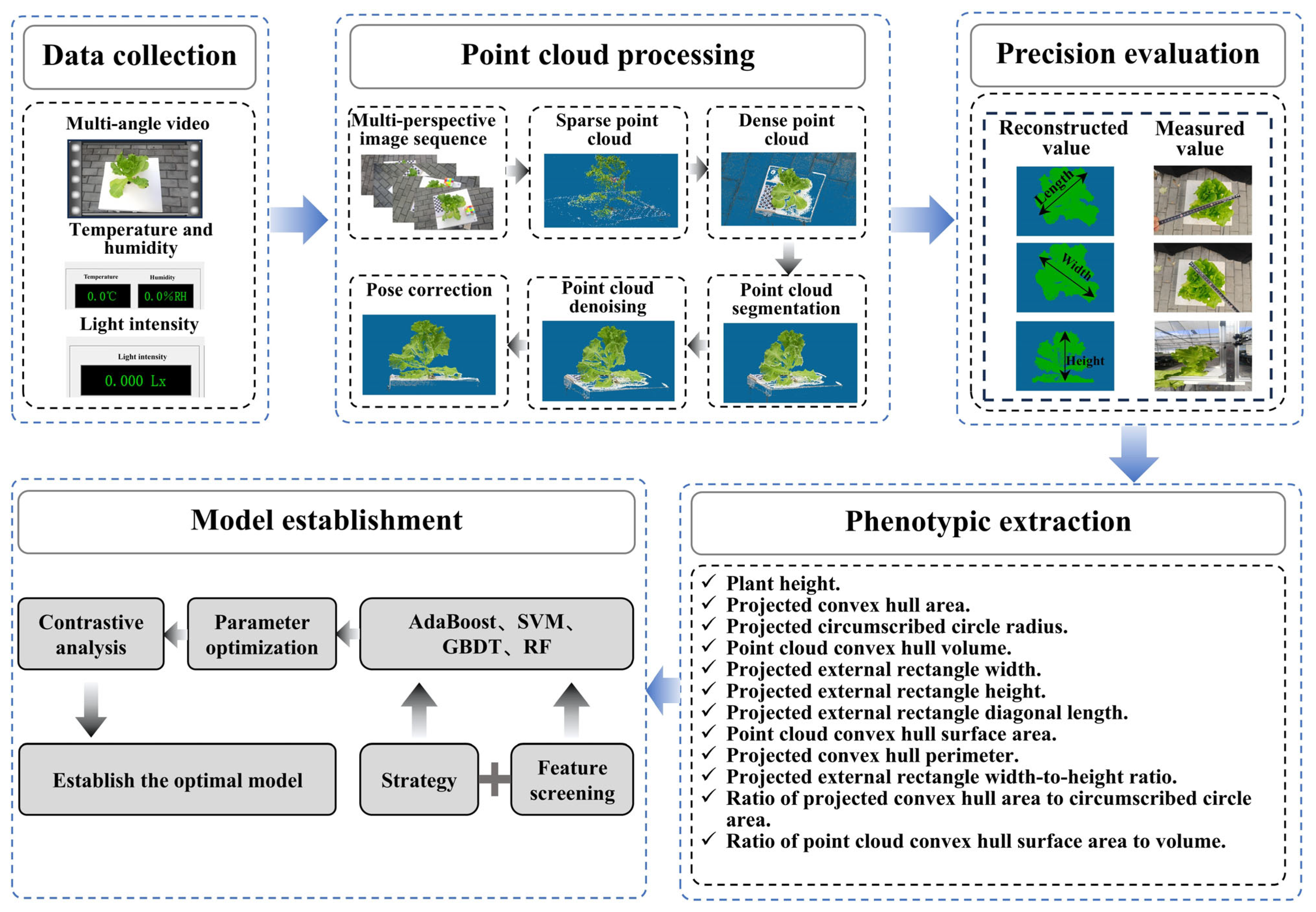
The phenotypic platform consists of three parts: an information collection module, a data collection system, and a data processing and phenotypic analysis system. The information collection module consists of a computer and a handheld information collection device. The data collection system controls the information collection module to collect the phenotypic information of lettuce and environmental parameters. The data processing and phenotyping system can extract frame images from multi-view video sequences, reconstruct the 3D point cloud structure of lettuce, extract key phenotypic parameters, and construct a biomass estimation model in combination with machine learning algorithms, as shown in Figure 2. The hardware environment used for data processing and phenotypic analysis in this study was an Intel (R) Core (TM) i9-13900HX CPU @2.20 GHz (Intel Corp., Santa Clara, CA, USA), NVIDIA GeForce GTX 4060 GPU, 32 GB of Samsung memory (Samsung Corp., Seoul, Republic of Korea), and a 2TB HP hard disk drive (HP Corp., Palo Alto, CA, USA), with the Windows 11 operating system.

The crop phenotype information collection device consists of two parts, as shown in Figure 3. Figure 3a is mainly a data collection hardware integration module, including parts a1, a2, and a3. a1 is a sensor and power supply unit integration module for handheld inspection devices, with a built-in RGB sensor (AT-36, Shenzhen Andong Electronic Development Co., Shenzhen, China), light sensor (B-RS-L30, Huai’an Blue Control Electronic Technology Co., Huai’an, China), and power supply unit. a2 is a handle that connects a1 and a3, which is easy to operate during information collection and is hollow inside, which is convenient for wiring. a3 is the base part, which supports the device parking, and installs the temperature and humidity sensor on the upper surface (B-TH-RS30, Huai’an Blue Control Electronic Technology Co., Huai’an, China). The sensor was masked using a1, which effectively avoided measurement errors of environmental information caused by direct light. The base was treated with through holes for easy wiring, enabling communication and control with a computer. Figure 3b is the computer, which is used to manipulate the collection device.

The data collection system is connected to the collection device through a computer and is responsible for controlling the sensors for the collection of multi-view image sequences and environmental information.

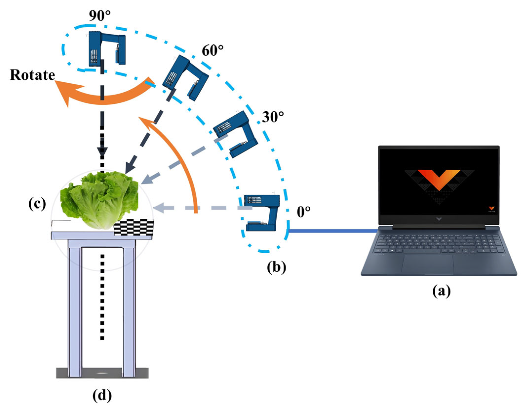
The collection process is shown in Figure 4. During the data collection process, the handheld detection device was located at the same level as the lettuce under test and maintained an appropriate distance to ensure that the crop was included in the field of view to the greatest extent during shooting; this initial position was defined as 0°. The computer sends commands to make the handheld detection device work, controlling the device to shoot 360° video data around the crop (Figure 4a).

Starting at 0° and gradually increasing to 90°, four location data collections were conducted (Figure 4b). The shooting time was 80 s per circle, with an interval of approximately 20 s, and the frame rate was 30 fps. For post-processing, an image was extracted at 25 frames, thereby extracting 24 images per circle at 15° intervals, and approximately 96 images were extracted for each plant, with an image resolution of 3840 × 2160. Meanwhile, the device collects environmental information in real time, including temperature, humidity, and light intensity.

2.3. Point Cloud Reconstruction

2.3.1. Overview of Point Cloud Processing Workflow

The three-dimensional reconstruction technique constructs three-dimensional point cloud models from 2D image sequences. First, the SFM algorithm is used for the sparse reconstruction of the image sequence. The process is based on a key point detection algorithm to extract the image features and match them, and estimate the attitude and position parameters of the camera based on the geometric constraint conditions between the images, thereby generating a sparse point cloud model of lettuce. Subsequently, based on the local photometric consistency and global consistency constraints, the MVS algorithm is used to densely reconstruct the calibrated image sequences, achieving the densification of sparse point clouds. Second, the actual scale is calculated using the checkerboard grid calibration method, and the dense point cloud is dimensionally calibrated. The point cloud is projected onto each coordinate plane, and a rotational transformation is performed based on the projection results, enabling the lettuce point-cloud model to be adjusted to the standard perspective. Finally, the phenotypic parameters of the lettuce are extracted from the adjusted point cloud based on the optimized phenotype extraction algorithm.

2.3.2. SFM-MVS Reconstruction

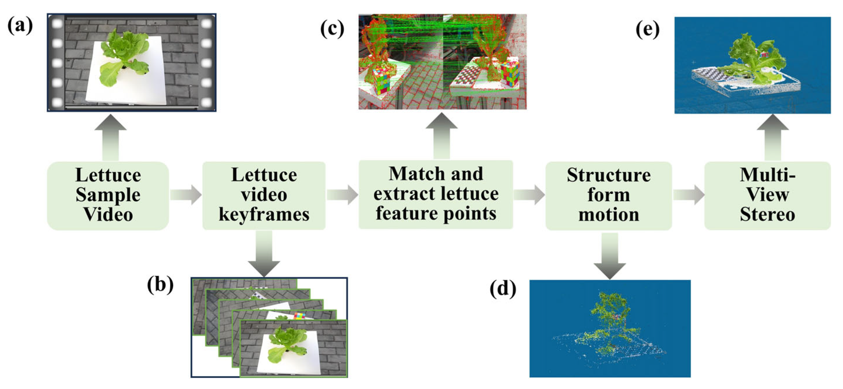
COLMAP (Version: 3.9.1) is a computer software developed and maintained by Stanford University, USA [40,41]. The software uses SVM and MVS algorithms, which are capable of reconstructing 3D point clouds from unordered or ordered image sequences and estimate camera poses. Therefore, this study used COLMAP for the 3D reconstruction of the lettuce samples, as shown in Figure 5. First, the lettuce samples were recorded on video using a handheld detection device (Figure 5a), followed by the extraction of image frames from the video (Figure 5c), and the extraction and matching of feature points (Figure 5b). Then, the sparse point cloud was reconstructed using the SFM algorithm (Figure 5d), and dense reconstruction using the MVS algorithm (Figure 5e), thereby achieving the densification of sparse point clouds.

2.3.3. Point Cloud Preprocessing

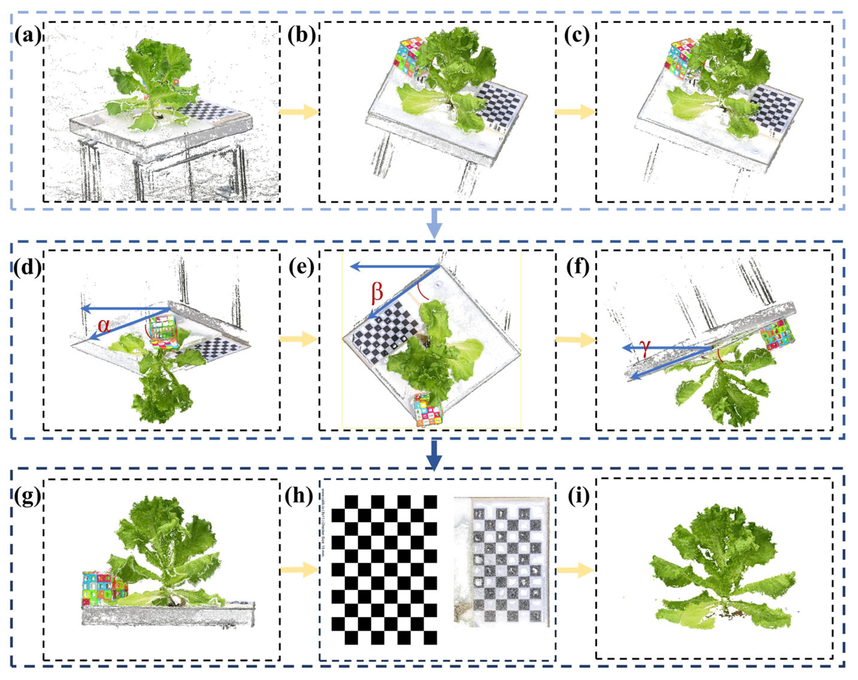
The point cloud data generated by the SFM-MVS algorithm is affected by factors such as camera position, shooting angle, and plant size, leading to the generation of point cloud data containing a large amount of background information and certain noise. Therefore, in this study, the reconstructed point cloud data needs to be preprocessed to preserve the 3D point cloud data of lettuce. The specific processing flow is illustrated in Figure 6.

Considering the presence of a large amount of background information in the original point cloud (Figure 6a), straight-pass filtering is used to remove the invalid background information. Specifically, first, a dimension and the value range under the dimension are specified. Second, each point in the point cloud is traversed to determine whether the value of the point in the specified dimension is within the value range. The points whose values are not within the value range are deleted. At the end of the traversal, the points left behind constitute the filtered point cloud (Figure 6b). The calculation formula is shown in Equation (1), as follows.

$$\left\{\begin{array}{c}{X}_a\le X\le X_b\\ Y_a\le Y\le Y_b\\ Z_a\le Z\le Z_b\end{array}\right.,$$

(1)

where ($X_a$, $X_b$), ($Y_a$, $Y_b$), and ($Z_a$, $Z_b$) represent the limited range of the lettuce point cloud on the $X$, $Y$, and $Z$ coordinate axes.

During the data collection process, due to factors such as background interference and environmental complexity, the generated point cloud data usually contain a large number of noisy points and outliers. To improve the accuracy of late phenotype extraction, this study employed the Statistical Outlier Removal (SOR) algorithm to process the noisy and outlier points near the lettuce point cloud [42]. The algorithm performed a statistical analysis of the neighborhood of each point and calculated the average distance from the point to its neighboring points. If it followed a Gaussian distribution, it was identified as an outlier, thereby achieving the identification and removal of outliers (Figure 6c).

Owing to the camera position, there was a deviation between the lettuce point cloud coordinate system and the desired coordinate system. To ensure the accuracy of subsequent processing, it is necessary to calibrate the coordinate system. First, the lettuce point clouds were projected onto the xoy, yoz, and xoz planes to obtain the corresponding projected point clouds (Figure 6d–f). Next, the projected point clouds on these three planes were analyzed to compute their tilt angles $\alpha$, $\beta$, and $\gamma$ with respect to the x-, y-, and z-axes. Then, the rotation matrices $R_x\left(\alpha \right)$, $R_y\left(\beta \right)$, and $R_z\left(\gamma \right)$ are constructed around the x-, y-, and z-axes, respectively. The integrated rotation matrix $R$ was obtained by multiplying these three rotation matrices. Finally, by applying a rotational transformation to the point cloud, it was transformed to the target pose, thereby constructing the corrected lettuce point cloud (Figure 6g). The specific calculations are shown in Formula (2)–(5).

$$R_x\left(\alpha \right)=\left[\begin{array}{ccc}1& 0& 0\\ 0& \mathit{cos}\left(\alpha \right)& -\mathit{sin}\left(\alpha \right)\\ 0& \mathit{sin}\left(\alpha \right)& \mathit{cos}\left(\alpha \right)\end{array}\right],$$

(2)

$$R_y\left(\beta \right)=\left[\begin{array}{ccc}\mathit{cos}\left(\beta \right)& 0& \mathit{sin}\left(\beta \right)\\ 0& 1& 0\\ -\mathit{sin}\left(\beta \right)& 0& \mathit{cos}\left(\beta \right)\end{array}\right],$$

(3)

$$R_z\left(\gamma \right)=\left[\begin{array}{ccc}\mathit{cos}\left(\gamma \right)& -\mathit{sin}\left(\gamma \right)& 0\\ \mathit{sin}\left(\gamma \right)& \mathit{cos}\left(\gamma \right)& 0\\ 0& 0& 1\end{array}\right],$$

(4)

$$R=R_x\left(\alpha \right) \ast R_y\left(\beta \right) \ast R_z\left(\gamma \right),$$

(5)

where $R_x\left(\alpha \right)$, $R_y\left(\beta \right),$ and $R_z\left(\gamma \right)$ are the rotation matrices of the lettuce point cloud around the x-, y-, and z-axes, respectively; $R$ is the integrated rotation matrix of the lettuce point cloud; and $\alpha$, $\beta$, and $\gamma$ are the rotation angles of the lettuce point cloud around the x-, y-, and z-axes, respectively.

Compared to sensors such as LiDAR or depth cameras, the results of point cloud generation based on MVS technology are affected by multiple factors, such as plant size, shooting position, camera angle, and camera configuration [43]. Owing to the discrepancy between the dimensions of the lettuce point cloud model on the standard spatial scale and the actual crop, to ensure the accuracy of the subsequent phenotypic analysis, this study used a checkerboard grid to correct the dimensions of the lettuce point cloud model. The specific implementation is as follows: based on the checkerboard grid point cloud data with known dimensions and the dimensions of the reconstructed checkerboard grid point cloud model, the scaling factor $M$ of the lettuce point cloud is determined according to Equation (6) (Figure 6h).

$$M=X/Y,$$

(6)

where $X$ and $Y$ are the actual and reconstructed dimensions of the lettuce sample, respectively, and $M$ is the scaling factor of the lettuce point cloud.

During the data collection process, the presence of the fixed plate significantly interfered with the extraction of lettuce phenotypic information. To effectively eliminate this interference, we adopted a method of extraction based on the color point clouds. The method identifies and preserves the key color features of lettuce while eliminating the interfering data of other colors. By implementing this strategy, we can eliminate the interference of the fixed plate on the point cloud data and retain the point cloud information of the lettuce completely, thus obtaining highly accurate 3D reconstruction results of the plant (Figure 6i).

Through the above processing, the point cloud data of lettuce plants were successfully extracted, thereby laying a reliable data foundation for subsequent phenotypic analysis.

2.4. Phenotypic Traits Extraction Methods

Previous studies have shown that morphological parameters of vegetation have a critical influence on its growth, development, and biomass prediction [44,45]. The distinctive features of a plant’s appearance accurately reflect its growth status. In particular, the expansion of the canopy structure is usually accompanied by an increase in photosynthetic efficiency, which promotes the synthesis and storage of organic matter [46]. Based on this, there is a clear correlation between external plant morphology and biomass production. In the modeling process, screening morphological parameters that have a decisive influence on biomass accumulation can significantly improve the stability and reliability of predictive models. In this study, the main morphological indicators of 12 crops and their derived variables, as shown in

Table 1. Phenotypic parameters used in this study and their abbreviations.

Phenotypic Parameters	Abbreviations
Plant height	PH
Projected convex hull area	PCHA
Projected circumscribed circle radius	PCCR
Point cloud convex hull volume	PCCHV
Projected external rectangle width	PER-W
Projected external rectangle height	PER-H
Projected external rectangle diagonal length	PER-DL
Point cloud convex hull surface area	PCCHSA
Projected convex hull perimeter	PCHP
Projected external rectangle width-to-height ratio	PER-WHR
Ratio of projected convex hull area to circumscribed circle area	PCHA/CCA
Ratio of point cloud convex hull surface area to volume	PCCHSA/PCCHV

, were systematically collected to assess crop biomass. These morphological parameters were incorporated into the model input variables for an in-depth study, validated by comparison, and finally filtered out the most contributing characteristic indicators for biomass estimation. The specific calculations for each parameter are as follows:

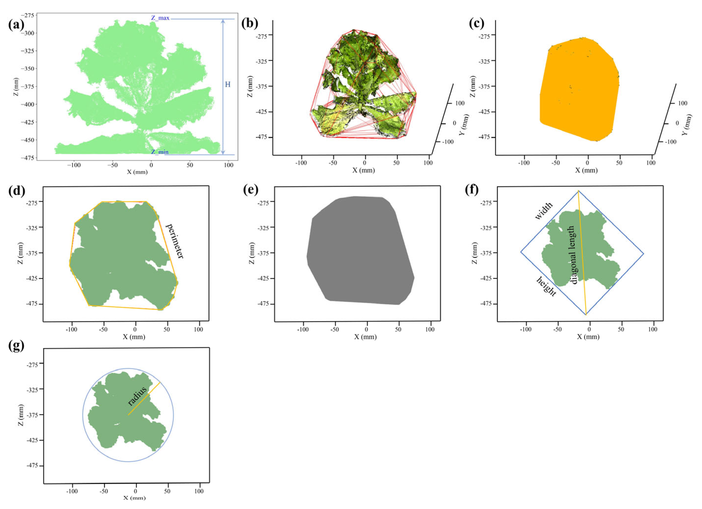
Plant height is an important component of plant structure that directly affects crop yield and quality [28,47]. The height of the lettuce plant was derived by calculating the difference between the maximum and minimum values of the point cloud data on the Z-axis coordinates, as shown in Figure 7a.

The volume and surface area of the convex hull are often used to characterize the overall size and growth of plants. The surface area and volume of plants are closely related to their photosynthetic capacity [48]. A larger surface area and volume means that the plant receives more light, thereby increasing the efficiency of photosynthesis and contributing to the accumulation of plant biomass [49]. In this study, a point-by-point analysis of the target point cloud was performed to construct a minimum convex polygonal bounding box to outline the plant shape, as shown in Figure 7b. The closed area formed by the minimally convex polygonal enclosing frame is the convex hull volume, and the triangular facets of the lettuce point cloud convex hull are traversed. The area of each triangular facet was computed and totaled to obtain the surface area of the lettuce point cloud convex hull, as shown in Figure 7c.

To further obtain additional phenotypic parameters, the 3D point cloud data was projected onto the xoy plane to generate 2D point cloud data. Using the Convex Hull function in the Scipy library, the convex hull of the two-dimensional point set was calculated based on the Qhull algorithm, and the vertex set of the minimum convex polygon containing all points was obtained. By traversing the convex hull vertices, by calculating the Euclidean distance between adjacent vertices on the convex hull boundary, and accumulating all the distance values, the projected convex hull perimeter was obtained, as shown in Figure 7d. Traversing the convex hull vertices, cross-multiply each vertex coordinate with the next vertex coordinate in order, add up all the results, take the absolute value and divide by 2 to get the projected convex hull area, as shown in Figure 7e. The extreme difference of the convex hull point set in the post-rotation x-axis projection is calculated as the projected external rectangle width, the extreme difference of the post-rotation y-axis projection is calculated as the projected external rectangle height, and the diagonal length of the external rectangle is calculated as the projected external rectangle diagonal length, as shown in Figure 7f. By calculating the Euclidean distance from the vertex of each convex hull to the center of mass, the maximum value obtained was the radius of the projected circumscribed circle radius, as shown in Figure 7g.

2.5. Dataset Exploration

The Pearson correlation coefficient (PCC) is an important indicator for measuring the degree of linear correlation between two variables; PCC values range from −1 to 1. The closer the PCC value is to 1, the stronger the positive correlation; the closer the PCC value is to −1, the stronger the negative correlation; and the closer the PCC value is to 0, the closer there is no correlation between the two variables. Figure 8 shows the correlation matrix between the 12 phenotypic parameters and lettuce biomass, demonstrating the relationship between the features in detail. The results show that there is a highly significant positive correlation (PCC ≥ 0.95) between the projected convex hull area, the point cloud convex hull surface area, and the projected convex hull perimeter, indicating that with an increase in the projected convex hull area, the point cloud convex hull surface area and the projected convex hull perimeter increase subsequently. The correlation coefficients of all three parameters with lettuce biomass were higher than 0.90, indicating that they were also significantly correlated with biomass. In addition, there was a negative correlation (PCC = −0.4) between the ratio of point cloud convex hull surface area to volume and biomass, meaning that as the ratio of point cloud convex hull surface area to volume increased, biomass decreased. Correlations between biomass and potential predictors showed that the features used to estimate biomass had the highest predictive power, namely the projected convex hull area, point cloud convex hull surface area, and projected convex hull perimeter, making it an important choice for predicting biomass. However, there were also high correlations between the rest of the input variables and the biomass. Because the input variables were all morphological parameters extracted from the reconstructed three-dimensional structure, the covariance level between the features was high, and it was difficult to effectively screen the input features using a single Pearson correlation coefficient. Therefore, an algorithm that was less sensitive to multiple covariances and combined with the SHAP technology was chosen to screen the input features of the biomass.

2.6. Biomass Estimation Modeling Methods

In this study, considering the small size of the lettuce sample dataset and the high correlation of the input variables, we selected Adaptive Boosting (AdaBoost), Gradient Boosting Decision Tree (GBDT), Support Vector Regression (SVR), and Random Forest Regression (RFR), four algorithms that are less sensitive to multicollinearity, to construct the prediction model for lettuce biomass. These machine learning methods have a significant advantage when dealing with small data samples and can improve the accuracy of predictions through algorithm optimization and adjustment. These methods also exhibit strong robustness to feature covariance. AdaBoost, GBDT, and RFR all belong to the integrated tree model based on decision trees. RFR trains multiple decision trees by randomly selecting samples and feature subsets through the bagging strategy, which effectively reduces the influence of covariance features on the model and outputs the results using a voting mechanism. GBDT adopts an iterative optimization approach to gradually fit the feature contributions and integrate the information of covariate features into the tree structure, thereby reducing the variance of parameter estimation. AdaBoost utilizes low-complexity decision tree stumps to focus on key information by adjusting the weights of the samples to weaken covariate interference. In contrast, SVR maps the data to a high-dimensional space through the kernel function with the goal of maximizing the spacing, which is insensitive to the linear correlation between the features, and effectively decouples the covariate features from their potential correlations. Compared with traditional linear regression, these machine learning methods do not require preprocessing of the covariate features, can directly utilize the intrinsic connection between the features to provide richer information for lettuce biomass prediction, and show good adaptability and high efficiency in small-sample scenarios.

In terms of model parameter configuration, GridSearch with 5-fold cross-validation was used for hyperparameter optimization. The key parameter search range was set, and all parameter combinations were traversed using GridSearchCV with R² as the optimization objective. The optimal parameter combination for the validation set was finally selected, as shown in

Table 2. List of ML algorithms and related hyperparameters used in this study.

ML Method	Features	List of Hyperparameters and Their Optimal Value
RFR	3 features	{‘max_depth’: None, ‘max_features’: None, ‘min_samples_leaf’: 2, ‘min_samples_split’: 3, ‘n_estimators’: 200}
	6 features	{‘max_depth’: 5, ‘max_features’: None, ‘min_samples_leaf’: 1, ‘min_samples_split’: 3, ‘n_estimators’: 200}
	12 features	{‘max_depth’: 5, ‘max_features’: None, ‘min_samples_leaf’: 1, ‘min_samples_split’: 2, ‘n_estimators’: 50}
GBDT	3 features	{‘learning_rate’: 0.05, ‘max_depth’: 5, ‘max_features’: ‘sqrt’, ‘n_estimators’: 100, ‘subsample’: 0.7}
	6 features	{‘learning_rate’: 0.1, ‘max_depth’: 3, ‘max_features’: ‘sqrt’, ‘n_estimators’: 200, ‘subsample’: 0.7}
	12 features	{‘learning_rate’: 0.05, ‘max_depth’: 5, ‘max_features’: ‘sqrt’, ‘n_estimators’: 100, ‘subsample’: 0.7}
SVR	3 features	{‘C’: 100, ‘degree’: 2, ‘epsilon’: 0.2, ‘gamma’: ‘scale’, ‘kernel’: ‘linear’}
	6 features	{‘C’: 10, ‘degree’: 2, ‘epsilon’: 0.5, ‘gamma’: 0.1, ‘kernel’: ‘rbf’}
	12 features	{‘C’: 100, ‘degree’: 2, ‘epsilon’: 0.2, ‘gamma’: ‘scale’, ‘kernel’: ‘linear’}
AdaBoost	3 features	{‘learning_rate’: 1, ‘loss’: ‘square’, ‘n_estimators’: 50}
	6 features	{‘learning_rate’: 0.1, ‘loss’: ‘square’, ‘n_estimators’: 50}
	12 features	{‘learning_rate’: 0.01, ‘loss’: ‘linear’, ‘n_estimators’: 50}

, and the remaining parameters were set as default. The optimal biomass estimation model was selected by comparing the performance of the four algorithms in lettuce biomass prediction.

To ensure that the model had good generalization performance and to avoid overfitting, this study adopted a random division method to divide the original dataset into a training set (70%) and a test set (30%). The training set was used for the optimization and learning of the model parameters, and the test set was used to evaluate the final performance of the model. In the model construction stage, four machine learning models, AdaBoost, GBDT, SVR, and RFR, were selected to construct the prediction model of lettuce biomass. To enhance the reliability of the model evaluation, 5-fold cross-validation was introduced in the experiment to test the stability and generalization ability of each model.

2.7. Performance Evaluation Metrics

To verify the accuracy of the 3D reconstruction and the validity of biomass prediction in this study, the coefficient of determination (R²) and root mean square error (RMSE) were used as assessment indices for the accuracy of phenotype extraction and biomass prediction. The calculation formulas are as follows:

$$R^2=1-{\displaystyle \frac{{\sum }_{i=1}^n{\left(y_i-{\widehat{y}}_i\right)}^2}{{\sum }_{i=1}^n{\left(y_i-{\overline{y}}_i\right)}^2}},$$

(7)

$$RMSE=\sqrt{{\displaystyle \frac{1}{n}}\sum _{i=1}^n{\left(y_i-{\widehat{y}}_i\right)}^2},$$

(8)

where $y_i$ is the actual measured value of the $i$th lettuce, ${\widehat{y}}_i$ is the predicted value of the $i$th lettuce, $\overline{y}$ is the mean of the actual measured value of the lettuce, and $n$ is the number of samples in the lettuce test set.

In order to further eliminate the influence of not using the range of sample values on the error indicator, this paper introduces the normalized root mean square error (RMSEn) to supplement the biomass prediction accuracy; the calculation formula is as follows:

$$RMSEn=100\times {\displaystyle \frac{RMSE}{max\left(y_i\right)-min\left(y_i\right)}},$$

(9)

where $max\left(y_i\right)$ and $min\left(y_i\right)$ denote the maximum and minimum values in the measured biomass values of lettuce, respectively. A smaller RMSEn indicates higher model prediction accuracy. In addition, for RMSEn values less than 10%, between 10% and 20%, between 20% and 30%, and more than 30%, the model simulations were considered excellent, good, fair, and poor, respectively [50].

2.8. Parameter Importance Analysis

When developing aboveground biomass prediction models, selecting the most relevant predictors is critical for improving the accuracy, reducing noise, and optimizing computational efficiency [51]. Shapley Added substance clarifications (SHAP), an advanced machine learning interpretability method, is often widely used to assess the contribution of various types of input features to the model prediction results, which significantly improves the interpretability of the model and thus optimizes the process of predictor screening. In this study, the introduction of the SHAP technique not only ensures the accuracy of the model prediction but also considers its interpretability and promotes the improvement of the predictor selection strategy. By accurately identifying the factors that are most influential in biomass prediction, SHAP can effectively eliminate redundant or irrelevant variables and focus on features that truly drive prediction. This approach significantly enhances the interpretability of machine-learning models and has demonstrated its value in multiple research areas and industrial practices [52,53]. SHAP analysis was performed using the Python package SHAP(Version: 0.47.2). Before implementing SHAP analysis, the variables were standardized and transformed, a preprocessing step that significantly reduced the interference of data scale differences in the assessment of SHAP values.

3. Results

3.1. Comparison of Multi-View Imaging and Light Field Imaging

To evaluate the reconstruction performance, this study used data collected by a light-field camera as a reference to compare the performance of a multi-view imaging system in the 3D reconstruction of individual lettuce plants. Data collection was conducted at the single plant level.

First, multi-view imaging devices were used to capture multi-view images of five pots of lettuce, followed by scanning the same plants with a light-field camera. The reconstruction quality was evaluated by comparing the point cloud data generated by the two methods [3]. Figure 9 shows the results of the point cloud visualization of the same plant using both methods. The experimental results showed that the point cloud data from multi-view imaging performed well in the RGB images of the corresponding viewpoints and accurately reproduced the vein characteristics and complex geometry of the edges of lettuce leaves (Figure 9a). This result is consistent with the advantages of multi-view imaging in terms of global structure recovery and texture preservation [54,55]. In contrast, the 3D visualization of the reconstructed point cloud by multi-view imaging was generally consistent with the point cloud data generated by the light-field imaging system (Figure 9b). However, the light-field imaging system requires complex calibration before 3D imaging and has high requirements for lighting conditions, resulting in a phenomenon where the point cloud appears darker in color. Despite the small number of missing localized regions in the multi-view imaging-reconstructed point cloud, the average relative error of the reconstruction (2.12%) was slightly lower than that of the light-field imaging system (2.74%) when compared with the measured values. Therefore, the multi-view imaging platform excels in reconstruction precision, reproduction of color texture and geometric morphological details, and requires no complex calibration and low operating costs.

3.2. Evaluation of Phenotypic Data

To verify the effectiveness of the information obtained by the device, we measured 64 reconstructed plants of Italian lettuce varieties at maturity, and the correlation between the reconstructed and true values was analyzed. Because the true values of plant height, crown height, and crown width can be obtained by manual measurement, the reconstruction results can be compared and analyzed. To evaluate the effectiveness of the device in obtaining information, the coefficient of determination (R²) and root mean square error (RMSE) were used as the evaluation metrics in this study. A linear correlation was established between the calculated and true values, and the results are shown in Figure 10.

The experimental results showed that the R² of lettuce plant height, crown height, and crown width reached 0.98, 0.99, and 0.99, respectively, and their RMSE values were 2.26 mm, 1.74 mm, and 1.69 mm, respectively, and the reconstruction error was consistently controlled within 2.26 mm. In addition, the fitted lines between the measured and predicted values of lettuce plant height, crown height, and crown width almost completely coincided with the 1:1 line, which fully proved the high accuracy of the 3D reconstruction of lettuce. Based on the above results, the image collection device adopted in this study demonstrated minimal error and high accuracy in reconstructing the three-dimensional model of lettuce and could achieve accurate acquisition of phenotypic data.

3.3. SHAP Analysis Results

Figure 11 shows the results of the SHAP summary analysis for the four integrated regression models, which visually presents the extent to which each input variable contributes to the model’s predictions. As shown in Figure 11a, the average SHAP values assigned to each input variable by each of the four integrated models reflected the average degree of contribution of these variables to the model output. The study used the top 50% features as screening thresholds, and by comparing the SHAP analysis results of the four machine learning methods, it was found that three features, PCHA, PCCHSA, and PCHP, were identified as key variables in all models, suggesting that they are decisive for biomass prediction. For example, PCHA is able to show the projected area of the plant canopy, a feature that reflects the efficiency of light energy capture in the three-dimensional space of the canopy, which plays an important role in relation to biomass accumulation. This finding matches the results of previous Pearson correlation analyses, in which the correlation coefficients for all three features exceeded 0.90, further confirming their centrality in the predictive model.

The frequency of occurrence of the three features, PCCHV, PH, and PER-W, in the importance assessment reached 0.75, indicating that they had a moderate impact on the predictive efficacy of the model. This finding is consistent with the results of the previous Pearson correlation analysis, where all three correlation coefficients with biomass were in the 0.80 to 0.90 range, confirming the complementary value of these traits in the biomass prediction models. Specifically, the PCCHV metric reflects the overall volume of the plant, and its value is positively correlated with plant weight, whereas PH and PER-W characterize morphological parameters such as plant height and width, respectively, and both of these characteristics are significantly associated with biomass estimation. A comprehensive analysis of multiple dimensions of plant morphology is expected to further improve the accuracy of prediction models.

By synthesizing the four models, it was found that predictors such as PCCR, PER-H, and PCHA/CCA had relatively low importance for biomass prediction, and their average SHAP values were significantly low. This result is consistent with the findings of a previous Pearson correlation study, where the correlation coefficients between these factors and biomass were approximately 0.5, indicating a weak correlation. From the perspective of model construction, these features may not have a significant correlation or even the possibility of redundancy, and their role in improving prediction accuracy is limited.

The results of the comprehensive SHAP evaluation show that the improvement in AGB estimation accuracy mainly relies on the significant role of key features, such as PCHA, PCCHSA, and PCHP, compared to the low contribution features, such as PCCR, PER-H, and PCHA/CCA, which can be eliminated, simplifying the calculation process and maintaining the prediction effect. By prioritizing high-impact variables, the SHAP-based screening strategy optimizes model efficacy and simultaneously enhances the accuracy and explanatory power of AGB predictions.

In Figure 11b, the point cloud distribution of the feature importance based on the SHAP method reveals the contribution of each variable to the predictive model and its interaction effect. The results of this visualization not only clearly present the degree and direction of the contribution of the features to the prediction results but also reveal the potential correlation between the features. Each data point in the point cloud represents the SHAP value of a specific feature in a single sample and characterizes the change in the feature value using a color gradient, where the blue to red color scale corresponds to a range of feature values from low to high. It is observed that the red-labeled points are generally distributed in the right region, indicating a positive contribution to the model output, while the blue-labeled points show a negative contribution. The results of the analysis showed that the high-value domains of PCHA had a significant correlation with larger predicted values, which implies that it plays a key role in the prediction process. Similarly, high PCCHSA values showed stable associations with positive SHAP values in all model constructs, confirming its importance as a key predictor. Although the extent of PCHP’s contribution of PCHP to most models was slightly weaker than that of PCHA and PCCHSA, it still proved to be an indispensable component of the prediction system. In contrast, the point clouds of features such as PCCR, PER-H, and PCHA/CCA are mainly clustered around the zero point, and their SHAP values are generally low, reflecting the fact that these variables have a negligible effect on the model output and are less susceptible to disturbances caused by fluctuations in the feature values.

3.4. Biomass Prediction Based on Machine Learning Algorithms

To assess the prediction accuracy of lettuce biomass, four machine learning algorithms, namely, Random Forest Regression (RFR), Gradient Boosting Decision Tree (GBDT), Support Vector Regression (SVR), and Adaptive Boosting (AdaBoost), were selected for this study to perform the modeling analysis. The performances of the models under different combinations of features were systematically compared by three evaluation metrics: normalized root mean square error (RMSEn), root mean square error (RMSE), and coefficient of determination (R²). The scatter plots presented in Figure 12 reflect the prediction effects under the full and filtered feature sets and visualize the degree of correlation between the model output values and the measured values. The experimental data show that the prediction accuracies of all models are maintained at a high level, in which the coefficient of determination R² is distributed in the range of 0.88–0.93, while the root mean square error RMSE is between 2.11–2.82 g, which confirms that the prediction results are in significant agreement with the true values. The normalized root mean square error RMSEn was in the range of 7.63–10.20% and all models accurately simulated biomass.

Random Forest Regression: As shown in Figure 12, R² is located at approximately 0.90, and the predicted scatter is tightly clustered around the 1:1 regression line with a narrow error band. The random forest regression model is naturally adapted to nonlinear interactions through multitree integration with random feature sampling. As the number of feature variables increased, the R² pair remained at approximately 0.90, indicating that the random forest exhibited strong robustness to feature redundancy. The model has excellent accuracy in simulating biomass and its RMSEn value is always around 9.50%.

Gradient Boosting Decision Tree: at 3–6 feature inputs, the R² is about 0.88, and at 12 feature inputs, the R² improves to 0.93, indicating that as the number of features increases, GBDT regression is able to effectively overcome the defect of the limited performance of the base learner at low-dimensional inputs. GBDT By optimizing the residuals through serialized fitting with higher-order feature combinations, the algorithm exhibits superior generalization performance.

Support Vector Regression: The predicted samples showed a wide, discrete distribution. For the R² value of 0.91 when three independent variables were used, although it showed that the model had some explanatory power, the discrete pattern of observations around the regression line suggests the inadequacy of the method in resolving the nonlinear associations between lettuce phenotypic traits and biomass. This result is consistent with the findings of Dhawi et al.; the poor fitness of the kernel function to complex interactions may affect the prediction accuracy [51]. When the number of independent variables was increased to six, R² slightly improved to 0.92; when it was increased to 12, R² decreased to 0.90, indicating that high-dimensional data are prone to trigger overfitting problems, reflecting the limitations of the method in complex feature interactions. The model performance was relatively better only when the feature dimensions were low, the linear relationship was significant, and there was no multicollinearity.

Adaptive Boosting: Under the conditions of 3, 6, and 12 features, its prediction accuracy is inferior to that of the comparison model, and the prediction points are discrete. The algorithm is iteratively optimized by a weak learner, but in the low-dimensional (3 features) case, the weak learner has difficulty in effectively identifying the key parameter associations; when the feature dimension is increased (12 features), the weak learner is not enough to deal with the complex interactions, and instead, it exacerbates the phenomenon of overfitting, resulting in the attenuation of the prediction performance.

The comparative analysis in Figure 12 shows that even with the simplified RFR model, the predictive efficacy is still significant and highly consistent with the measured aboveground biomass data. Under the premise that the feature variables have been optimized and screened, the predictive accuracy of the model does not show significant attenuation, which proves that the streamlined feature combination still has strong explanatory power. This feature makes it particularly suitable for applications where data resources are limited or where the focus is on model simplicity. In biomass prediction, the RFR model showed optimal performance with a significant correlation between its predictions and measured data, while maintaining a low error level, which makes it ideal for simplifying the model construction process.

3.5. Evaluating and Comparing Machine Learning Models for Estimating Aboveground Biomass

Table 3. Prediction results for different feature combinations.

Features	ML Model	R2 (Train)	RMSE (g) (Train)	RMSEn (%) (Train)	R2 (Test)	RMSE (g) (Test)	RMSEn (%) (Test)
3 features	RFR	0.97	1.42	4.94	0.90	2.63	9.53
	GBDT	0.99	0.25	0.88	0.88	2.82	10.20
	SVR	0.90	2.62	9.10	0.91	2.40	8.68
	AdaBoost	0.97	1.37	4.76	0.89	2.79	10.09
6 features	RFR	0.98	1.07	3.70	0.90	2.58	9.34
	GBDT	0.99	0.02	0.06	0.88	2.81	10.19
	SVR	0.94	2.01	6.99	0.92	2.32	8.40
	AdaBoost	0.98	1.25	4.34	0.89	2.73	9.87
12 features	RFR	0.98	1.16	4.01	0.90	2.63	9.53
	GBDT	0.99	0.17	0.58	0.93	2.11	7.63
	SVR	0.92	2.39	8.29	0.90	2.59	9.38
	AdaBoost	0.98	1.23	4.27	0.89	2.69	9.74

provides a comparative analysis report of four machine learning models: Random Forest Regression (RFR), Gradient Boosting Decision Tree (GBDT), Support Vector Regression (SVR), and Adaptive Boosting (AdaBoost), with different feature inputs: three significant features, six most significant features, and all features.

For 3 features: the SVR regression achieved the highest accuracy (R² = 0.91, RMSE = 2.40 g, RMSEn = 8.68%), followed by the RFR regression (R² = 0.90, RMSE = 2.63 g, RMSEn = 9.53%) and the AdaBoost regression (R² = 0.89, RMSE = 2.79 g, RMSEn = 10.09%), and the GBDT regression was poor (R² = 0.88, RMSE = 2.82 g, RMSEn = 10.20%). These results show that SVR in this scenario can effectively utilize a limited set of three features to capture the potential relationships predicted by AGB, which demonstrates some advantages in dealing with small-scale feature combinations.

For 6 features: Among the models with six input features, SVR still leads (R² = 0.92, RMSE = 2.32 g, RMSEn = 8.40%), RFR maintains a stable accuracy (R² = 0.90, RMSE = 2.58 g, RMSEn = 9.34%), AdaBoost performs similarly to the state with three features (R² = 0.89, RMSE = 2.73 g, RMSEn = 9.87%), and GBDT has a small increase in performance but is still not as good as SVR (R² = 0.88, RMSE = 2.81 g, RMSEn = 10.19%). The results illustrate that when the number of features is moderately increased, SVR can further mine the feature information to enhance the prediction accuracy, and the other models have relatively limited gains from additional features.

For 12 features: when using the 12 input features, GBDT emerged as the best performer, achieving a high level of accuracy (R² = 0.93, RMSE = 2.11 g, RMSEn = 7.63%); RFR maintained a consistent accuracy (R² = 0.90, RMSE = 2.63 g, RMSEn = 9.53%); and SVR performance decreased slightly but remained at a better level (R² = 0.90, RMSE = 2.59 g, RMSEn = 9.38%); AdaBoost maintained the previous performance trend (R² = 0.89, RMSE = 2.69 g, RMSEn = 9.74%). This shows that the GBDT can fully utilize the rich information in the 12 feature sets through its gradient boosting framework and shows strong adaptability to complex feature interactions, which is in line with the characteristics of the gradient boosting class of models that are suitable for handling high-dimensional feature scenarios.

Compared to single features, multivariate feature combinations were more effective in predicting biomass, a finding that is consistent with the conclusion of Tatsumi et al. that multivariate features enhance prediction performance [56]. Specifically, when the number of features in the GBDT model was increased to 12, its ability to parse the nonlinear relationships between features was significantly enhanced, which in turn led to a substantial improvement in prediction accuracy. Dhakal et al. study confirmed that the synergistic effect of integrated spectral, morphological, and textural features can effectively optimize biomass estimation results [57]. The multi-parameter fusion strategy of PCHA, PCCHSA, and PCHP used in this paper constructs a more complete data dimension for biomass prediction. Related studies have pointed out that height and canopy geometric parameters (e.g., projected convex hull area) play a key role in biomass prediction models as plant-related variables [58,59]. The introduction of these canopy structure features significantly improved the model estimation accuracy.

4. Discussion

4.1. Relationship Between Morphological Structure and Biomass

The phenotypic characteristics of the above-ground parts of plants serve as a direct physical basis for biomass accumulation, and their accurate acquisition is crucial for biomass prediction. These phenotypic parameters regulate the spatial allocation and radiation-use efficiency of photosynthetic organs in space and respond to environmental variations through plastic phenotypes, thereby altering biomass allocation mechanisms and output levels [7,8,9]. At the same time, the structural characteristics of plants reflect to a certain extent their adaptive strategies to the environment, dynamically adjusting organ configurations in response to environmental gradients in order to optimize the efficiency of the absorption and utilization of light energy, water, and mineral elements, and ultimately regulating the process of biomass formation [13,14,15]. The structural features of plant canopies can provide three-dimensional canopy information and better reflect canopy growth and biomass. Many studies have validated the potential of structural features in biomass estimation [57,60]. Xiao et al. [61] utilized morphological traits such as convex hull volume and total leaf area of sugar beet for biomass prediction, and the results showed that these traits had strong correlations with biomass, with R² of 0.78–0.88. Therefore, the accurate collection of plant phenotypic traits is decisive for improving the reliability of yield prediction. In this study, we used a multi-view image fusion method to establish a three-dimensional digital model to determine both plant height and canopy projected area, and to obtain spatial occupancy and canopy morphological features, thus achieving a complete characterization of the morphological structure of lettuce [62,63,64]. This method improves the measurement accuracy of the conformational parameters to more than 0.98, providing highly accurate data support for phenotypic prediction models.

4.2. Key Morphological Feature Extraction and Modeling Strategies

The accuracy of biomass estimation is highly dependent on the reasonable selection of characteristic variables, and scientific screening of characteristic parameters is the key to improving prediction efficiency. In this study, the random forest regression method was used to compare and analyze three, six, and twelve characteristic variables as model inputs. The experimental results show that when all 12 features are directly used to construct the RFR model, its prediction performance is not significantly improved with an increase in the number of features, and the coefficient of determination, R², is always stable at approximately 0.90. This indicates that the number of feature parameters is not as high as the better, and in biomass estimation, too many feature inputs may lead to a less efficient model.

By calculating the Pearson correlation coefficients for the geometric features, significant multicollinearity between the predictor variables was observed. This result was expected because most morphological parameters were calculated based on three-dimensional structural features. If all the strongly correlated variables are included in the regression model simultaneously, it will lead to data duplication, which in turn will cause fluctuations in the parameter estimates. To address this problem, we considered an integrated machine-learning algorithm. By analyzing the SHAP values of all variables, the contribution of biomass can be visualized and ranked, thus effectively solving the problem of the covariance of multiple input features. This mechanism significantly improves the interpretability of the machine learning model, enhances its credibility and reliability in practical applications, and provides an effective way to deeply understand the decision logic of the model. When ranking SHAP variables, the machine learning algorithm does not eliminate any predictors with correlation, nor does it select only a single relevant variable, but ensures that predictors with multicollinearity can still participate in model building by reasonably assigning weights to each variable. This approach is effective in avoiding the omission of biologically important variables [65]. Therefore, it is crucial to select key morphological features to estimate the biomass.

The structural features identified with high criticality through SHAP analysis have demonstrated certain application potential. For instance, the three key feature variables, PCHA, PCCHSA, and PCHP, can effectively evaluate the horizontal coverage capability and canopy structure compactness of plants, which are closely linked to light interception efficiency and growth potential. These features can be used as a basis for early screening of robust plants. PCHA, PCCHSA, and PCHP reflect the plant’s capacity for spatial expansion and vertical growth, aiding in the assessment of individual competitiveness and resource utilization efficiency under dense planting conditions. The biomass prediction models constructed based on these morphological characteristics facilitate precise management in greenhouses and the formulation of high-yield cultivation strategies. They also provide a reliable basis for the classification of lettuce quality grades and the screening of germplasm resources. During the breeding process, the key structural features identified through these models offer criteria for the early selection of phenotypically superior lines, enhancing breeding efficiency and shortening the screening cycle.

4.3. Performance Comparison of Different Machine Learning Models

In this study, we adopted a 7:3 training–test split strategy to prevent model overfitting and used the performance of the test set as the primary evaluation criterion to more objectively reflect the generalization ability of the model on unknown samples. To further analyze the fitting ability and stability of the model, we not only introduced 5-fold cross-validation to enhance the stability of the training process, but also systematically compared the performance differences of different models and feature combinations on the training set and test set (see Table 3). The results showed that the difference between the training and test R² values of most models was within a reasonable range, and no obvious overfitting phenomenon occurred. Although some feature combinations performed well on the training set, they showed certain performance decline on the test set, which might be related to the small sample size and limited data distribution of the current dataset. Although this study incorporated cross-validation and independent test set division strategies during the modeling process to enhance the robustness of the model, the limited sample size may still affect the model’s generalization ability in large-scale datasets. Firstly, the current sample distribution in morphological features is relatively limited, which may not be sufficient to support the model’s adequate learning of extreme or atypical structures, thereby affecting its predictive performance in a wider range of phenotypic variations. Secondly, the model training is mainly based on lettuce samples, and different crops have significant differences in organ structure, spatial distribution, and phenotypic expression. Taking crops like corn and tomato, which have more complex three-dimensional structures or stronger organ dominance, for example, the completeness and stability of their three-dimensional structure reconstruction may be insufficient, and the robustness of the extracted features may also decline, thereby affecting the accuracy and universality of biomass estimation.

Parameter configuration is a crucial and indispensable step in optimizing model performance, and appropriate parameter settings can have a decisive impact on improving model effectiveness. By utilizing the grid search tuning technique, all potential combinations of preset input parameters can be systematically explored to obtain a more exhaustive search scope and ultimately determine an optimal solution.

For biomass prediction, the four models showed excellent performance for biomass simulation with a range of RMSEn of 7.63–10.20%. The Gradient Boosted Decision Tree (GBDT) model achieved the best performance under the combined characterization condition, with a coefficient of determination R² of 0.93 and a root mean square error of 2.11 g. The model optimizes residual fitting tree-by-tree through gradient iteration and deeply explores the interactions between high-dimensional features, thereby maximizing the algorithm’s predictive advantages in complex phenotypic regression problems. Random Forest Regression (RFR) showed outstanding performance in the feature screening process. Its mechanism, based on the integration of multiple decision trees, not only recognizes nonlinear associations among variables but also significantly reduces sensitivity to multicollinearity problems. This property enables the RFR to maintain reliable predictive stability when the computational conditions are restricted or the feature dimensions are low. In contrast, the AdaBoost algorithm has consistently low R² values under different feature input conditions, and the prediction results are more discrete. The model relies on the continuous learning of weak classifiers, which limits the learning ability when the number of features is insufficient, making it difficult to recognize the key parameter associations. When the number of features is too large, overfitting can easily occur because of the insufficient ability of weak classifiers to deal with complex interactions, which restricts the prediction accuracy. Support vector regression (SVR) is deficient in resolving nonlinear associations between phenotypic parameters and biomass, and the kernel function is poorly adapted to complex feature interactions, resulting in prediction results that are difficult to achieve the desired accuracy. In addition, numerous studies have demonstrated the significant advantages of random forest algorithms in carrying out biomass and yield modeling predictions for crops such as lettuce and wheat [66,67].

Although this study has employed classic machine learning methods such as Random Forest Regression (RFR), Gradient Boosting Decision Tree (GBDT), Support Vector Regression (SVR), and AdaBoost to model biomass and achieved stable prediction results under different feature combinations, it has not yet introduced the rapidly developing deep learning modeling frameworks, such as the Convolutional Neural Network (CNN) and Multi-Layer Perceptron (MLP). Compared with machine learning methods, these models demonstrate stronger stability in handling high-dimensional, nonlinear feature interaction relationships and large sample data. By introducing these modern modeling strategies, the applicability and robustness of biomass prediction models can be evaluated more comprehensively from multiple perspectives, such as accuracy, efficiency, and interpretability. However, due to the limited sample size of this study, deep learning methods are prone to overfitting in small sample scenarios, and the stability of model training is difficult to guarantee. Therefore, in this stage, they were not used as the core modeling tool. Nevertheless, their potential advantages are worth further verification and exploration in subsequent studies with expanded sample sizes.

4.4. Limitations and Future Work

This study still has deficiencies in the three-dimensional reconstruction and biomass estimation of lettuce. First, the detection device designed and constructed in this paper mainly conducted experiments on the Italian non-blotching lettuce variety under specific planting conditions. However, there were no experiments conducted on different varieties, different growth stages, and different planting environments. In the future, it is possible to explore the prediction of the growth status throughout the entire growth period. And under strong light irradiation, shadow occlusion, or complex backgrounds was not verified, and the subsequent verification work in complex environments can be increased. Meanwhile, multi-source data fusion or adaptive sampling techniques can be explored to improve the efficiency of 3D point cloud reconstruction in complex environments and to reduce data redundancy. Second, the RFR model showed high prediction precision (R² = 0.90) for biomass estimation in this experiment; however, its universality had not been verified. Subsequently, the detection of other vegetables can be increased, while the development of lightweight deep learning models or the introduction of incremental learning strategies can be considered to reduce the computational complexity and time cost, and improve the model’s adaptability to dynamic environmental conditions.

5. Conclusions

This study successfully constructed a non-destructive and portable plant 3D reconstruction and biomass detection device, which enabled the in situ collection and accurate analysis of crop phenotypic data.

In terms of 3D reconstruction and phenotypic extraction, this study adopted the SFM-MVS method for 3D reconstruction and preprocessed the 3D point cloud model using point cloud filtering, straight-pass filtering, and point cloud color extraction. These methods effectively removed background noise and redundant data, providing reliable data for subsequent phenotypic parameter extraction. The study extracted 12 phenotypic parameters, including plant height, crown length and width, and convex hull volume. The accuracy of plant height, crown height, and crown width was verified, and the results showed that R² was 0.98, 0.99, and 0.99, and RMSE was 2.26 mm, 1.74 mm, and 1.69 mm, respectively. The reconstructed 3D point cloud model has high precision and can accurately reflect the 3D morphology of the plant, providing a basis for biomass prediction and growth analysis.

In terms of biomass prediction, this study compared the prediction performances of four models, AdaBoost, SVR, GBDT, and RFR, under different feature inputs. By combining Pearson’s correlation coefficient and SHAP value analyses, we ranked the features in terms of their contribution, which improved the interpretability and transparency of the input features. By comparing the estimation accuracies of different feature combinations with the four machine learning regression models, we found that the RFR model can guarantee prediction accuracy and reduce feature inputs while maintaining a more stable prediction when only three features are used. This makes it an optimal estimation model.

In summary, this study proposes a multi-trait phenotypic analysis of lettuce based on SFM-MVS for facility lettuce and biomass detection. Through the organic combination of plant 3D reconstruction and biomass detection, we can accurately obtain multiple phenotypic parameters and biomass information of crops, providing a scientific basis for crop variety selection and intelligent management and control of facilities.

References

1. Diez, Y.; Kentsch, S.; Fukuda, M.; Caceres, M.L.L.; Moritake, K.; Cabezas, M. Deep learning in forestry using UAV-acquired RGB data: A practical review. Remote Sens. 2021, 13, 2837. [Google Scholar] [CrossRef]
2. Vázquez-Arellano, M.; Griepentrog, H.W.; Reiser, D.; Paraforos, D.S. 3-D imaging systems for agricultural applications—A review. Sensors 2016, 16, 618. [Google Scholar] [CrossRef] [PubMed]
3. Wang, Y.; Wen, W.; Wu, S.; Wang, C.; Yu, Z.; Guo, X.; Zhao, C. Maize plant phenotyping: Comparing 3D laser scanning, multi-view stereo reconstruction, and 3D digitizing estimates. Remote Sens. 2018, 11, 63. [Google Scholar] [CrossRef]
4. Kim, M.J.; Moon, Y.; Tou, J.C.; Mou, B.; Waterland, N.L. Nutritional value, bioactive compounds and health benefits of lettuce (Lactuca sativa L.). J. Food Compos. Anal. 2016, 49, 19–34. [Google Scholar] [CrossRef]
5. Du, H.; Liu, L.; Su, L.; Zeng, F.; Wang, K.; Peng, W.; Zhang, H.; Song, T. Seasonal changes and vertical distribution of fine root biomass during vegetation restoration in a karst area, Southwest China. Front. Plant Sci. 2019, 9, 2001. [Google Scholar] [CrossRef]
6. Wei, L.; Yang, H.; Niu, Y.; Zhang, Y.; Xu, L.; Chai, X. Wheat biomass, yield, and straw-grain ratio estimation from multi-temporal UAV-based RGB and multispectral images. Biosyst. Eng. 2023, 234, 187–205. [Google Scholar] [CrossRef]
7. Jin, X.; Zarco-Tejada, P.J.; Schmidhalter, U.; Reynolds, M.P.; Hawkesford, M.J.; Varshney, R.K.; Yang, T.; Nie, C.; Li, Z.; Ming, B. High-throughput estimation of crop traits: A review of ground and aerial phenotyping platforms. IEEE Geosci. Remote Sens. Mag. 2020, 9, 200–231. [Google Scholar] [CrossRef]
8. Sun, G.; Wang, X. Three-dimensional point cloud reconstruction and morphology measurement method for greenhouse plants based on the kinect sensor self-calibration. Agronomy 2019, 9, 596. [Google Scholar] [CrossRef]
9. Zhang, Y.; Li, M.; Li, G.; Li, J.; Zheng, L.; Zhang, M.; Wang, M. Multi-phenotypic parameters extraction and biomass estimation for lettuce based on point clouds. Measurement 2022, 204, 112094. [Google Scholar] [CrossRef]
10. Si, C.; Lin, Y.; Luo, S.; Yu, Y.; Liu, R.; Naz, M.; Dai, Z. Effects of LED light quality combinations on growth and leaf colour of tissue culture-generated plantlets in Sedum rubrotinctum. Hortic. Sci. Technol. 2024, 42, 53–67. [Google Scholar] [CrossRef]
11. Li, W.; Zhang, C.; Ma, T.; Li, W. Estimation of summer maize biomass based on a crop growth model. Emir. J. Food Agric. (EJFA) 2021, 33, 742–750. [Google Scholar] [CrossRef]
12. Tunio, M.H.; Gao, J.; Lakhiar, I.A.; Solangi, K.A.; Qureshi, W.A.; Shaikh, S.A.; Chen, J. Influence of atomization nozzles and spraying intervals on growth, biomass yield, and nutrient uptake of butter-head lettuce under aeroponics system. Agronomy 2021, 11, 97. [Google Scholar] [CrossRef]
13. Golbach, F.; Kootstra, G.; Damjanovic, S.; Otten, G.; van de Zedde, R. Validation of plant part measurements using a 3D reconstruction method suitable for high-throughput seedling phenotyping. Mach. Vis. Appl. 2016, 27, 663–680. [Google Scholar] [CrossRef]
14. Vulpi, F.; Marani, R.; Petitti, A.; Reina, G.; Milella, A. An RGB-D multi-view perspective for autonomous agricultural robots. Comput. Electron. Agric. 2022, 202, 107419. [Google Scholar] [CrossRef]
15. Rebetzke, G.; Jimenez-Berni, J.; Fischer, R.; Deery, D.; Smith, D. High-throughput phenotyping to enhance the use of crop genetic resources. Plant Sci. 2019, 282, 40–48. [Google Scholar] [CrossRef]
16. Grzybowski, M.; Wijewardane, N.K.; Atefi, A.; Ge, Y.; Schnable, J.C. Hyperspectral reflectance-based phenotyping for quantitative genetics in crops: Progress and challenges. Plant Commun. 2021, 2, 100209. [Google Scholar] [CrossRef]
17. Wang, J.; Zhang, Y.; Gu, R. Research status and prospects on plant canopy structure measurement using visual sensors based on three-dimensional reconstruction. Agriculture 2020, 10, 462. [Google Scholar] [CrossRef]
18. Ji, Y.; Chen, Z.; Cheng, Q.; Liu, R.; Li, M.; Yan, X.; Li, G.; Wang, D.; Fu, L.; Ma, Y. Estimation of plant height and yield based on UAV imagery in faba bean (Vicia faba L.). Plant Methods 2022, 18, 26. [Google Scholar] [CrossRef]
19. Zhu, W.; Feng, Z.; Dai, S.; Zhang, P.; Wei, X. Using UAV multispectral remote sensing with appropriate spatial resolution and machine learning to monitor wheat scab. Agriculture 2022, 12, 1785. [Google Scholar] [CrossRef]
20. Li, S.; Yan, Z.; Guo, Y.; Su, X.; Cao, Y.; Jiang, B.; Yang, F.; Zhang, Z.; Xin, D.; Chen, Q. SPM-IS: An auto-algorithm to acquire a mature soybean phenotype based on instance segmentation. Crop J. 2022, 10, 1412–1423. [Google Scholar] [CrossRef]
21. Akhtar, M.S.; Zafar, Z.; Nawaz, R.; Fraz, M.M. Unlocking plant secrets: A systematic review of 3D imaging in plant phenotyping techniques. Comput. Electron. Agric. 2024, 222, 109033. [Google Scholar] [CrossRef]
22. Qian, Y.; Xu, Q.; Yang, Y.; Lu, H.; Li, H.; Feng, X.; Yin, W. Classification of rice seed variety using point cloud data combined with deep learning. Int. J. Agric. Biol. Eng. 2021, 14, 206–212. [Google Scholar] [CrossRef]
23. Cao, W.; Zhou, J.; Yuan, Y.; Ye, H.; Nguyen, H.T.; Chen, J.; Zhou, J. Quantifying variation in soybean due to flood using a low-cost 3D imaging system. Sensors 2019, 19, 2682. [Google Scholar] [CrossRef] [PubMed]
24. Zhang, Y.; Teng, P.; Aono, M.; Shimizu, Y.; Hosoi, F.; Omasa, K. 3D monitoring for plant growth parameters in field with a single camera by multi-view approach. J. Agric. Meteorol. 2018, 74, 129–139. [Google Scholar] [CrossRef]
25. Nguyen, T.T.; Slaughter, D.C.; Max, N.; Maloof, J.N.; Sinha, N. Structured light-based 3D reconstruction system for plants. Sensors 2015, 15, 18587–18612. [Google Scholar] [CrossRef] [PubMed]
26. Patel, A.K.; Park, E.-S.; Lee, H.; Priya, G.L.; Kim, H.; Joshi, R.; Arief, M.A.A.; Kim, M.S.; Baek, I.; Cho, B.-K. Deep learning-based plant organ segmentation and phenotyping of sorghum plants using LiDAR point cloud. IEEE J. Sel. Top. Appl. Earth Obs. Remote Sens. 2023, 16, 8492–8507. [Google Scholar] [CrossRef]
27. Thapa, S.; Zhu, F.; Walia, H.; Yu, H.; Ge, Y. A novel LiDAR-based instrument for high-throughput, 3D measurement of morphological traits in maize and sorghum. Sensors 2018, 18, 1187. [Google Scholar] [CrossRef]
28. He, W.; Ye, Z.; Li, M.; Yan, Y.; Lu, W.; Xing, G. Extraction of soybean plant trait parameters based on SfM-MVS algorithm combined with GRNN. Front. Plant Sci. 2023, 14, 1181322. [Google Scholar] [CrossRef]
29. Wang, Y.; Hu, S.; Ren, H.; Yang, W.; Zhai, R. 3DPhenoMVS: A low-cost 3D tomato phenotyping pipeline using 3D reconstruction point cloud based on multiview images. Agronomy 2022, 12, 1865. [Google Scholar] [CrossRef]
30. Gu, W.; Wen, W.; Wu, S.; Zheng, C.; Lu, X.; Chang, W.; Xiao, P.; Guo, X. 3D Reconstruction of Wheat Plants by Integrating Point Cloud Data and Virtual Design Optimization. Agriculture 2024, 14, 391. [Google Scholar] [CrossRef]
31. Zhu, L.; Jiang, W.; Sun, B.; Chai, M.; Li, S.; Ding, Y. Three-dimensional Reconstruction and Phenotype Parameters Acquisition of Seeding Vegetables Based on Neural Radiance Fields. Trans. Chin. Soc. Agric. Mach. 2024, 55, 391. [Google Scholar]
32. Iglhaut, J.; Cabo, C.; Puliti, S.; Piermattei, L.; O’Connor, J.; Rosette, J. Structure from motion photogrammetry in forestry: A review. Curr. For. Rep. 2019, 5, 155–168. [Google Scholar] [CrossRef]
33. Hui, F.; Zhu, J.; Hu, P.; Meng, L.; Zhu, B.; Guo, Y.; Li, B.; Ma, Y. Image-based dynamic quantification and high-accuracy 3D evaluation of canopy structure of plant populations. Ann. Bot. 2018, 121, 1079–1088. [Google Scholar] [CrossRef] [PubMed]
34. Yang, C.; Sun, L.; Zhang, J.; Fan, X.; Zhang, D.; Ren, T.; Liu, M.; Zhang, Z.; Ma, W. Comprehensive Analysis of Phenotypic Traits in Chinese Cabbage Using 3D Point Cloud Technology. Agronomy 2024, 14, 2506. [Google Scholar] [CrossRef]
35. Wu, S.; Wen, W.; Wang, Y.; Fan, J.; Wang, C.; Gou, W.; Guo, X. MVS-Pheno: A portable and low-cost phenotyping platform for maize shoots using multiview stereo 3D reconstruction. Plant Phenomics 2020, 2020, 1848437. [Google Scholar] [CrossRef]
36. Bhuyan, B.P.; Tomar, R.; Singh, T.; Cherif, A.R. Crop type prediction: A statistical and machine learning approach. Sustainability 2022, 15, 481. [Google Scholar] [CrossRef]
37. Castillo-Botón, C.; Casillas-Pérez, D.; Casanova-Mateo, C.; Ghimire, S.; Cerro-Prada, E.; Gutierrez, P.A.; Deo, R.C.; Salcedo-Sanz, S. Machine learning regression and classification methods for fog events prediction. Atmos. Res. 2022, 272, 106157. [Google Scholar] [CrossRef]
38. Paidipati, K.K.; Chesneau, C.; Nayana, B.; Kumar, K.R.; Polisetty, K.; Kurangi, C. Prediction of rice cultivation in India—Support vector regression approach with various kernels for non-linear patterns. AgriEngineering 2021, 3, 182–198. [Google Scholar] [CrossRef]
39. Apergis, N.; Manickavasagam, J.; Visalakshmi, S. A novel hybrid approach to forecast crude oil futures using intraday data. Technol. Forecast. Soc. Change 2020, 158, 120126. [Google Scholar]
40. Schonberger, J.L.; Frahm, J.-M. Structure-from-motion revisited. In Proceedings of the IEEE Conference on Computer Vision and Pattern Recognition, Las Vegas, NV, USA, 27–30 June 2016; pp. 4104–4113. [Google Scholar]
41. Schönberger, J.L.; Zheng, E.; Frahm, J.-M.; Pollefeys, M. Pixelwise view selection for unstructured multi-view stereo. In Proceedings, Part III 14, Proceedings of the Computer Vision–ECCV 2016: 14th European Conference, Amsterdam, The Netherlands, 11–14 October 2016; Springer: Cham, Switzerland, 2016; pp. 501–518. [Google Scholar]
42. Jin, S.; Bi, H.; Feng, J.; Xu, W.; Xu, J.; Zhang, J. Research on 4-D Imaging of Holographic SAR Differential Tomography. Remote Sens. 2023, 15, 3421. [Google Scholar] [CrossRef]
43. Wu, S.; Wen, W.; Gou, W.; Lu, X.; Zhang, W.; Zheng, C.; Xiang, Z.; Chen, L.; Guo, X. A miniaturized phenotyping platform for individual plants using multi-view stereo 3D reconstruction. Front. Plant Sci. 2022, 13, 897746. [Google Scholar] [CrossRef]
44. Combs, T.P.; Didan, K.; Dierig, D.; Jarchow, C.J.; Barreto-Muñoz, A. Estimating Productivity Measures in Guayule Using UAS Imagery and Sentinel-2 Satellite Data. Remote Sens. 2022, 14, 2867. [Google Scholar] [CrossRef]
45. Guo, Y.; Schöb, C.; Ma, W.; Mohammat, A.; Liu, H.; Yu, S.; Jiang, Y.; Schmid, B.; Tang, Z. Increasing water availability and facilitation weaken biodiversity–biomass relationships in shrublands. Ecology 2019, 100, e02624. [Google Scholar] [CrossRef] [PubMed]
46. Vermeiren, J.; Villers, S.L.; Wittemans, L.; Vanlommel, W.; van Roy, J.; Marien, H.; Coussement, J.R.; Steppe, K. Quantifying the importance of a realistic tomato (Solanum lycopersicum) leaflet shape for 3-D light modelling. Ann. Bot. 2020, 126, 661–670. [Google Scholar] [CrossRef] [PubMed]
47. Niu, Y.; Han, W.; Zhang, H.; Zhang, L.; Chen, H. Estimating maize plant height using a crop surface model constructed from UAV RGB images. Biosyst. Eng. 2024, 241, 56–67. [Google Scholar] [CrossRef]
48. Jiao, Y.; Niklas, K.J.; Wang, L.; Yu, K.; Li, Y.; Shi, P. Influence of leaf age on the scaling relationships of lamina mass vs. area. Front. Plant Sci. 2022, 13, 860206. [Google Scholar] [CrossRef]
49. Dieleman, J.A.; De Visser, P.H.; Meinen, E.; Grit, J.G.; Dueck, T.A. Integrating morphological and physiological responses of tomato plants to light quality to the crop level by 3D modeling. Front. Plant Sci. 2019, 10, 839. [Google Scholar] [CrossRef]
50. Nasim, W.; Ahmad, A.; Belhouchette, H.; Fahad, S.; Hoogenboom, G. Evaluation of the OILCROP-SUN model for sunflower hybrids under different agro-meteorological conditions of Punjab—Pakistan. Field Crops Res. 2016, 188, 17–30. [Google Scholar] [CrossRef]
51. Dhawi, F.; Ghafoor, A.; Almousa, N.; Ali, S.; Alqanbar, S. Predictive modelling employing machine learning, convolutional neural networks (CNNs), and smartphone RGB images for non-destructive biomass estimation of pearl millet (Pennisetum glaucum). Front. Plant Sci. 2025, 16, 1594728. [Google Scholar] [CrossRef]
52. Parsa, A.B.; Movahedi, A.; Taghipour, H.; Derrible, S.; Mohammadian, A.K. Toward safer highways, application of XGBoost and SHAP for real-time accident detection and feature analysis. Accid. Anal. Prev. 2020, 136, 105405. [Google Scholar] [CrossRef]
53. Lim, B.; Zohren, S. Time-series forecasting with deep learning: A survey. Philos. Trans. R. Soc. A 2021, 379, 20200209. [Google Scholar] [CrossRef]
54. Santoši, Ž.; Budak, I.; Stojaković, V.; Šokac, M.; Vukelić, Đ. Evaluation of synthetically generated patterns for image-based 3D reconstruction of texture-less objects. Measurement 2019, 147, 106883. [Google Scholar] [CrossRef]
55. Li, Y.; Liu, J.; Zhang, B.; Wang, Y.; Yao, J.; Zhang, X.; Fan, B.; Li, X.; Hai, Y.; Fan, X. Three-dimensional reconstruction and phenotype measurement of maize seedlings based on multi-view image sequences. Front. Plant Sci. 2022, 13, 974339. [Google Scholar] [CrossRef] [PubMed]
56. Tatsumi, K.; Igarashi, N.; Mengxue, X. Prediction of plant-level tomato biomass and yield using machine learning with unmanned aerial vehicle imagery. Plant Methods 2021, 17, 77. [Google Scholar] [CrossRef]
57. Dhakal, R.; Maimaitijiang, M.; Chang, J.; Caffe, M. Utilizing spectral, structural and textural features for estimating oat above-ground biomass using UAV-based multispectral data and machine learning. Sensors 2023, 23, 9708. [Google Scholar] [CrossRef] [PubMed]
58. Cardenas-Gallegos, J.S.; Lacerda, L.N.; Severns, P.M.; Peduzzi, A.; Klimeš, P.; Ferrarezi, R.S. Advancing biomass estimation in hydroponic lettuce using RGB-depth imaging and morphometric descriptors with machine learning. Comput. Electron. Agric. 2025, 234, 110299. [Google Scholar] [CrossRef]
59. Yu, D.; Zha, Y.; Sun, Z.; Li, J.; Jin, X.; Zhu, W.; Bian, J.; Ma, L.; Zeng, Y.; Su, Z. Deep convolutional neural networks for estimating maize above-ground biomass using multi-source UAV images: A comparison with traditional machine learning algorithms. Precis. Agric. 2023, 24, 92–113. [Google Scholar] [CrossRef]
60. Viljanen, N.; Honkavaara, E.; Näsi, R.; Hakala, T.; Niemeläinen, O.; Kaivosoja, J. A novel machine learning method for estimating biomass of grass swards using a photogrammetric canopy height model, images and vegetation indices captured by a drone. Agriculture 2018, 8, 70. [Google Scholar] [CrossRef]
61. Xiao, S.; Chai, H.; Shao, K.; Shen, M.; Wang, Q.; Wang, R.; Sui, Y.; Ma, Y. Image-based dynamic quantification of aboveground structure of sugar beet in field. Remote Sens. 2020, 12, 269. [Google Scholar] [CrossRef]
62. Maimaitijiang, M.; Sagan, V.; Sidike, P.; Hartling, S.; Esposito, F.; Fritschi, F.B. Soybean yield prediction from UAV using multimodal data fusion and deep learning. Remote Sens. Environ. 2020, 237, 111599. [Google Scholar] [CrossRef]
63. Wan, L.; Cen, H.; Zhu, J.; Zhang, J.; Zhu, Y.; Sun, D.; Du, X.; Zhai, L.; Weng, H.; Li, Y. Grain yield prediction of rice using multi-temporal UAV-based RGB and multispectral images and model transfer—A case study of small farmlands in the South of China. Agric. For. Meteorol. 2020, 291, 108096. [Google Scholar] [CrossRef]
64. Zhao, Y.; Zhang, X.; Sun, J.; Yu, T.; Cai, Z.; Zhang, Z.; Mao, H. Low-cost lettuce height measurement based on depth vision and lightweight instance segmentation model. Agriculture 2024, 14, 1596. [Google Scholar] [CrossRef]
65. Cutler, D.R.; Edwards, T.C., Jr.; Beard, K.H.; Cutler, A.; Hess, K.T.; Gibson, J.; Lawler, J.J. Random forests for classification in ecology. Ecology 2007, 88, 2783–2792. [Google Scholar] [CrossRef]
66. Zhai, W.; Li, C.; Cheng, Q.; Mao, B.; Li, Z.; Li, Y.; Ding, F.; Qin, S.; Fei, S.; Chen, Z. Enhancing wheat above-ground biomass estimation using UAV RGB images and machine learning: Multi-feature combinations, flight height, and algorithm implications. Remote Sens. 2023, 15, 3653. [Google Scholar] [CrossRef]
67. Wengert, M.; Piepho, H.-P.; Astor, T.; Graß, R.; Wijesingha, J.; Wachendorf, M. Assessing spatial variability of barley whole crop biomass yield and leaf area index in silvoarable agroforestry systems using UAV-borne remote sensing. Remote Sens. 2021, 13, 2751. [Google Scholar] [CrossRef]
Figure 1. Lettuce growing environment.
Agriculture 15 01662 g001
Figure 2. Flow of lettuce 3D reconstruction and biomass determination.
Agriculture 15 01662 g002
Figure 3. Hardware structure diagram of the device. (a) Hardware integration module: a1 is the hardware composition of the upper part of the handheld device, a2 is the handle connector, and a3 is the support and hardware integration part of the base of the collection device; (b) computer: data collection control terminal.
Agriculture 15 01662 g003
Figure 4. Data acquisition workflow. (a) Data collection control terminal; (b) schematic of ring harvesting from 0° to 90°; (c) collection sample lettuce; and (d) support rack for storing collection samples.
Agriculture 15 01662 g004
Figure 5. Point cloud reconstruction workflow. (a) Video of lettuce samples recorded by the handheld detection device; (b) image sequence after video frame extraction and processing; (c) feature point matching between the two images; (d) sparse point clouds generated from image sequences; and (e) dense point cloud after processing using the dense reconstruction algorithm.
Agriculture 15 01662 g005
Figure 6. Lettuce point cloud preprocessing workflow. (a) Reconstruction of the original point cloud; (b) target point cloud obtained using conditional constraint segmentation; (c) point cloud processed by the SOR filtering algorithm; (d) projected point cloud after the target point cloud is projected onto the xoy plane; (e) projected point cloud after the target point cloud is projected onto the xoz plane; (f) projected point cloud after projection of the target point cloud to the yoz plane; (g) target point cloud after coordinate correction; (h) the checkerboard grid and its point cloud model for solving the scaling factor; and (i) lettuce point cloud after complete reconstruction.
Agriculture 15 01662 g006
Figure 7. Schematic diagram of phenotypic extraction. (a) Schematic diagram of plant height; (b) enclosed 3D convex envelope wireframe of the lettuce point cloud; (c) enclosed 3D convex hull area and volume of the lettuce point cloud; (d) convex hull perimeter of the projected point cloud; (e) convex hull area of the projected point cloud; (f) projected external width, height, and diagonal length of the projected point cloud; and (g) radius of the external circle of the projected point cloud.
Agriculture 15 01662 g007
Figure 8. Pearson correlation coefficients between features. Note: The color of the graph from light blue to purple indicates the correlation coefficient from −1 to 1; the numerical value in each cell indicates the Pearson correlation coefficient between the two, where values (0, 1) denote a positive correlation, and the closer the value is to 1, the stronger the co-directional variation between the two indicators; and (−1, 0) denotes a negative correlation, and the smaller the value, the more pronounced the decrease in one indicator when the other increases.
Agriculture 15 01662 g008
Figure 9. Comparison of point clouds obtained by light-field cameras and multi-view imaging. (a) Point clouds obtained by multi-view reconstruction; (b) point clouds acquired by light-field cameras.
Agriculture 15 01662 g009
Figure 10. Correlation between the measured and calculated values of plant height, crown height, and crown width; confidence interval (α) is 0.05. (a) Plant height; (b) canopy width; and (c) canopy height.
Agriculture 15 01662 g010
Figure 11. SHAP summary plot of four integrated regression models, showing the average contribution of features to the prediction of biomass. (a) Mean SHAP contribution ranking histogram: demonstrates the mean absolute SHAP value of each feature to biomass prediction, ranked from highest to lowest overall influence. Top-ranked features contribute more to the prediction; (b) SHAP feature importance point plot: demonstrates how individual feature points positively and negatively influence the model output, with the color band fading from blue to red, reflecting the change in magnitude of the feature values, and thus the actual degree of contribution of the input variables in the final prediction results.
Agriculture 15 01662 g011
Figure 12. Relationship between the predicted and measured biomass using four machine learning models. (a) Three features; (b) six features; and (c) twelve features.
Agriculture 15 01662 g012