

GDFC-YOLO: An Efficient Perception Detection Model for Precise Wheat Disease Recognition


Abstract
1. Introduction
2. Materials and Methods
2.1. Dataset Construction
2.1.1. Data Sources
2.1.2. Dataset Production
2.2. YOLOv11 Convolutional Neural Network
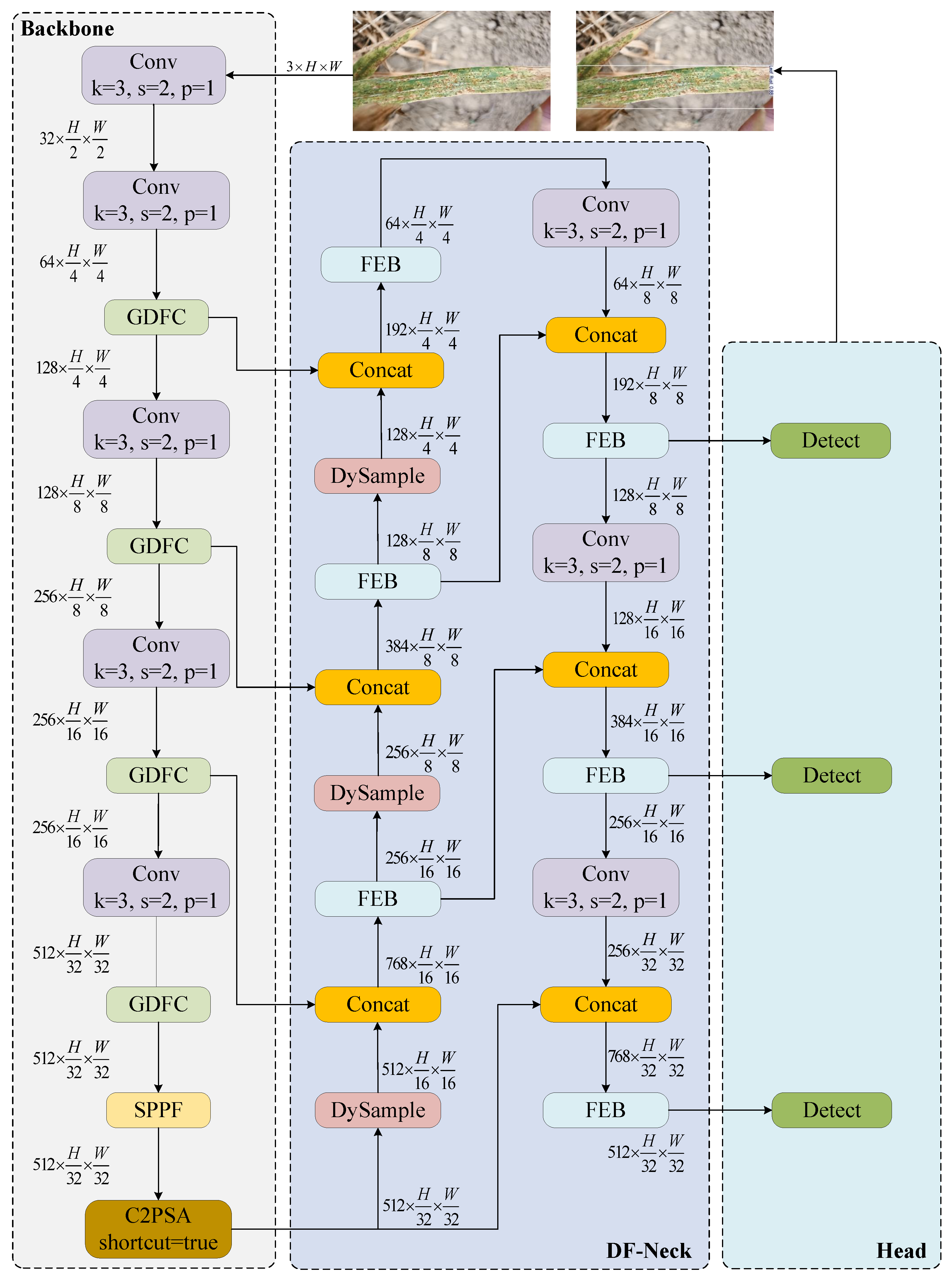
2.3. YOLOv11 Network Improvements
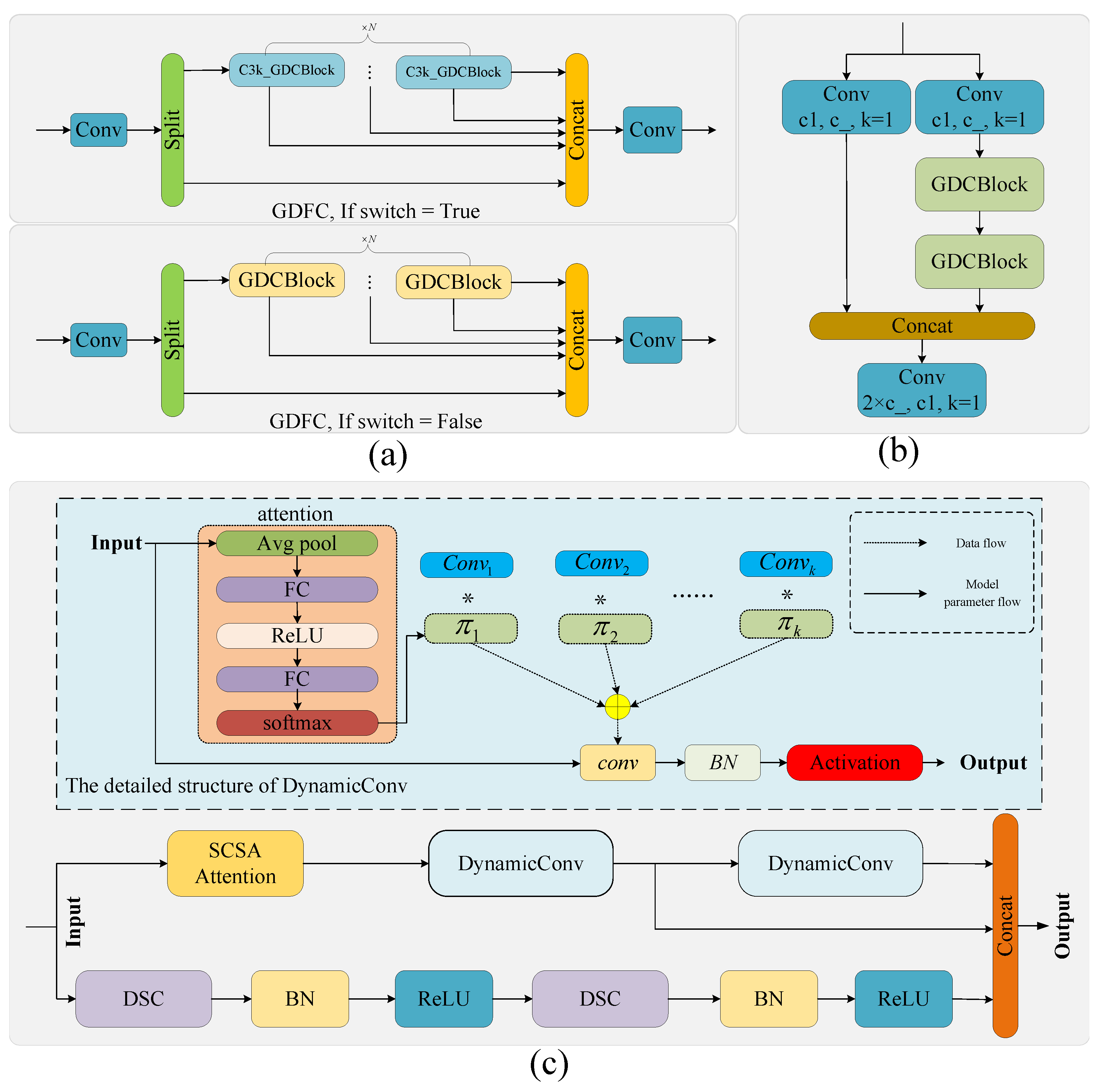
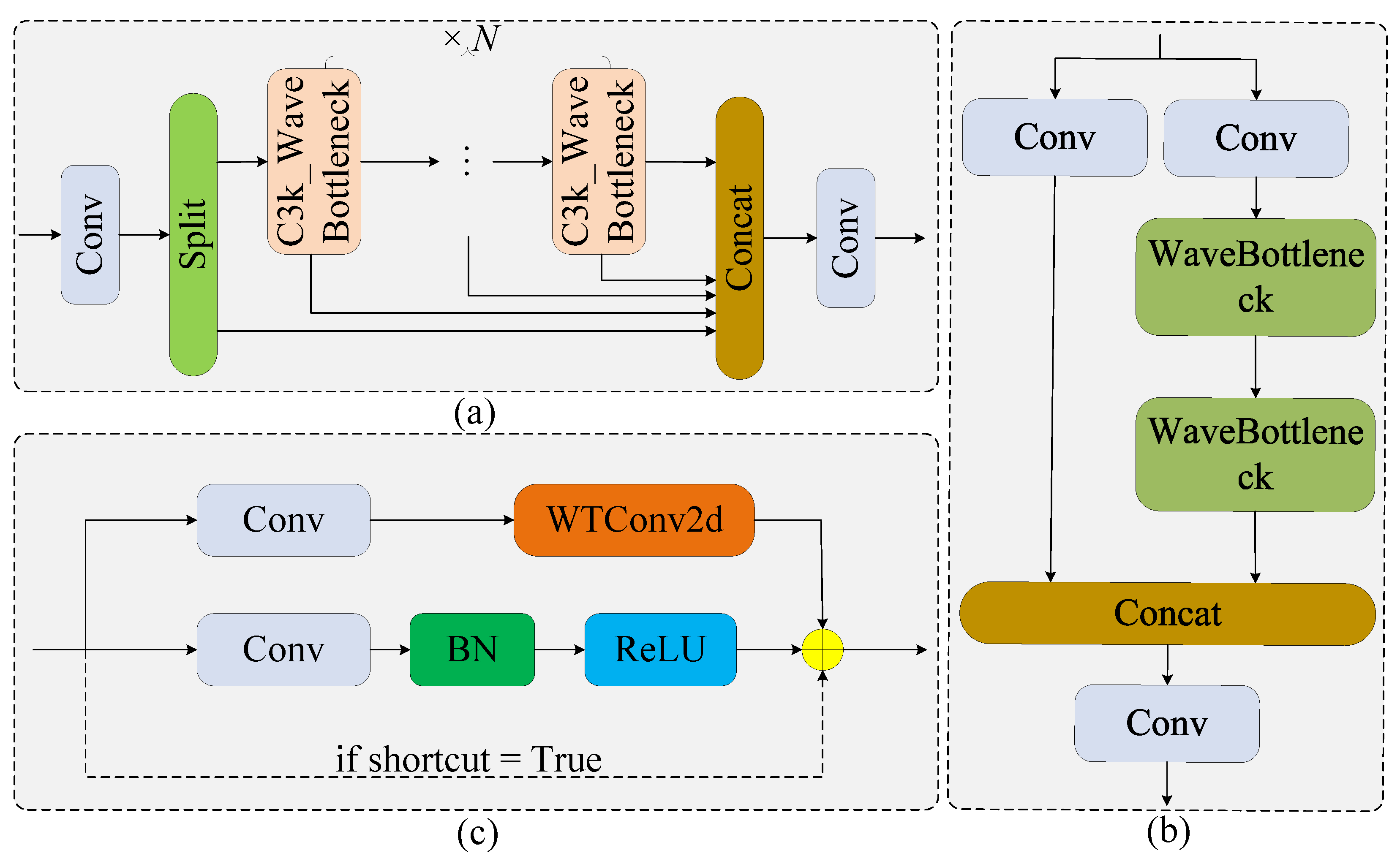
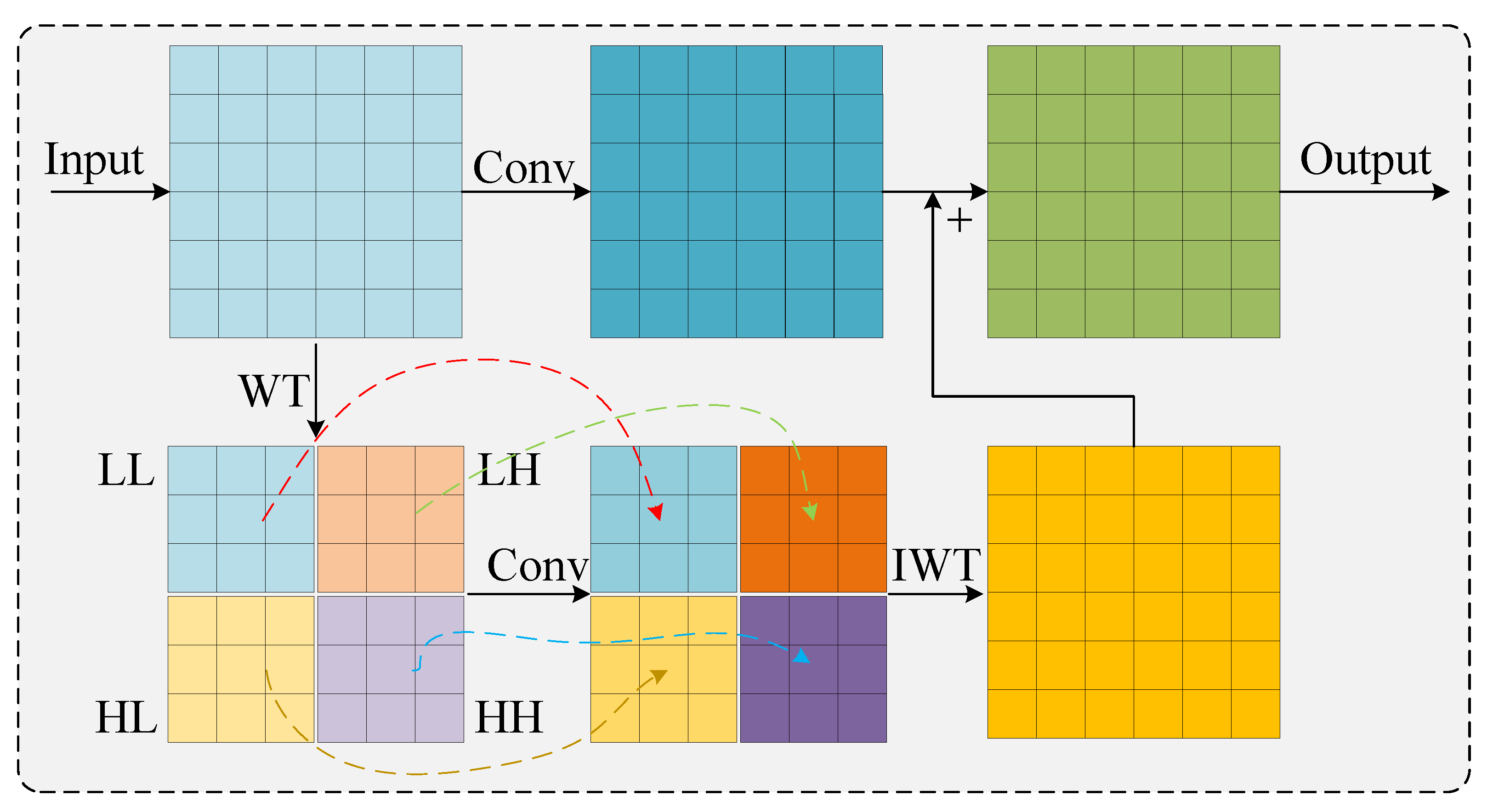
2.3.1. Ghost Dynamic Feature Core
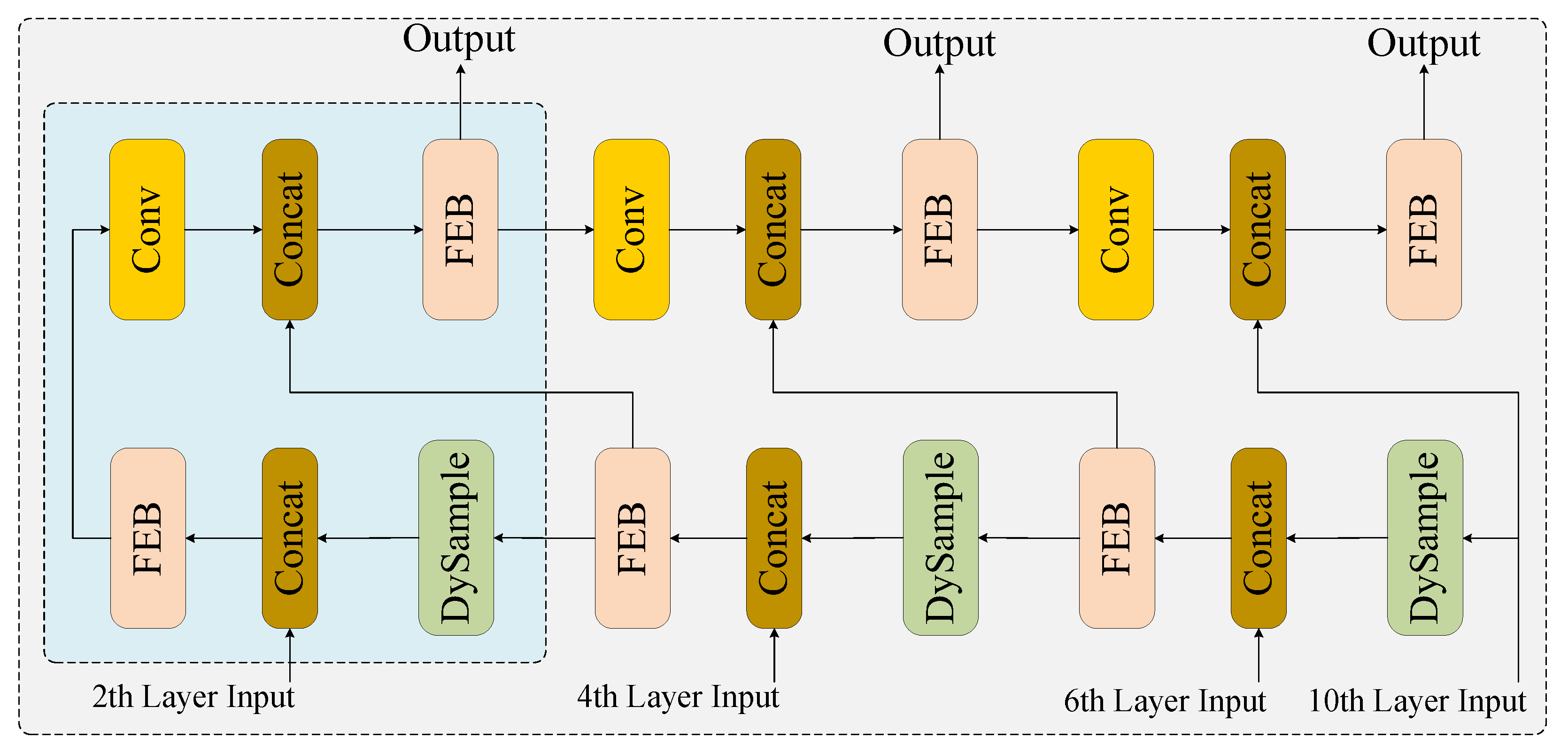
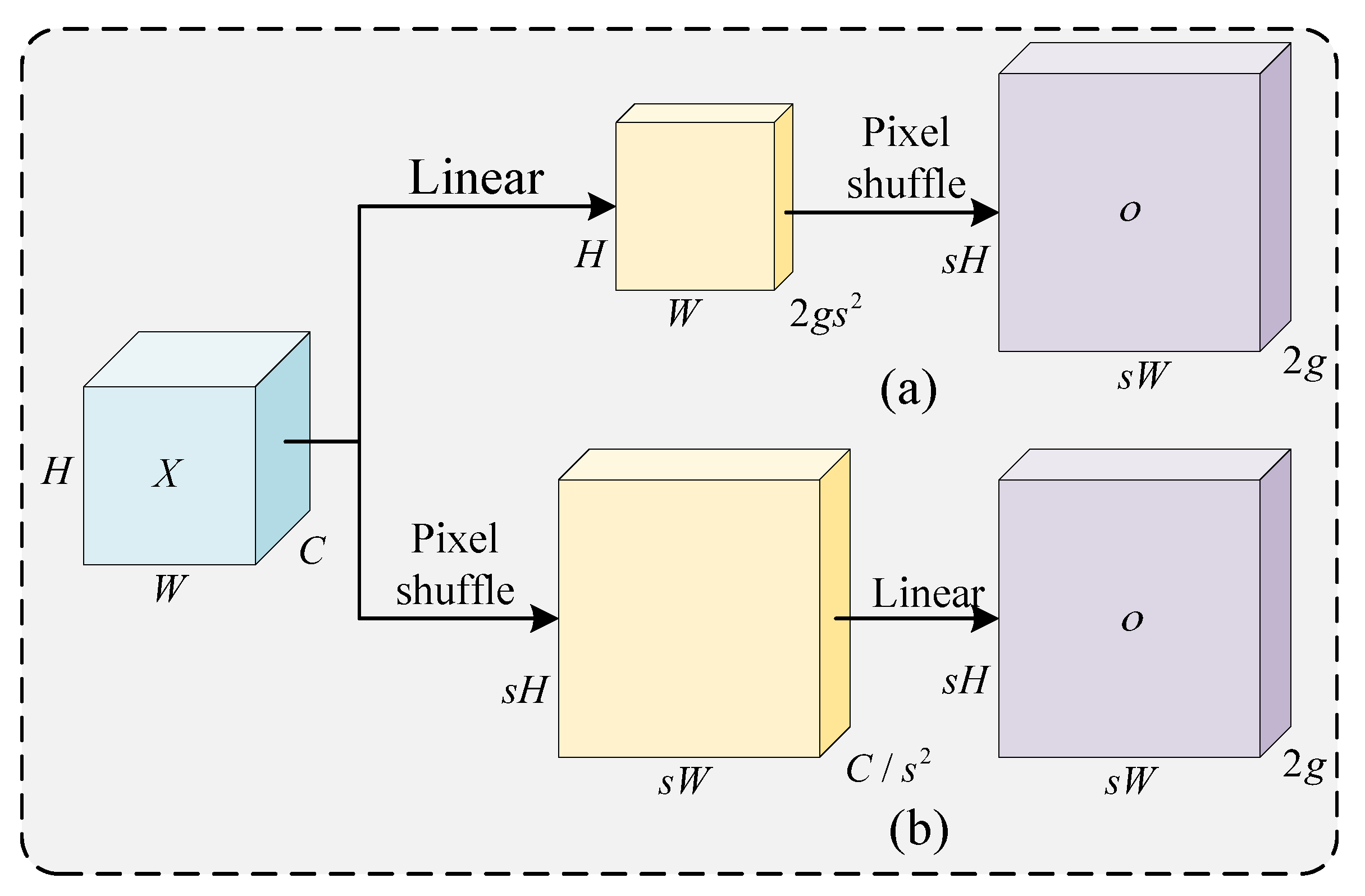
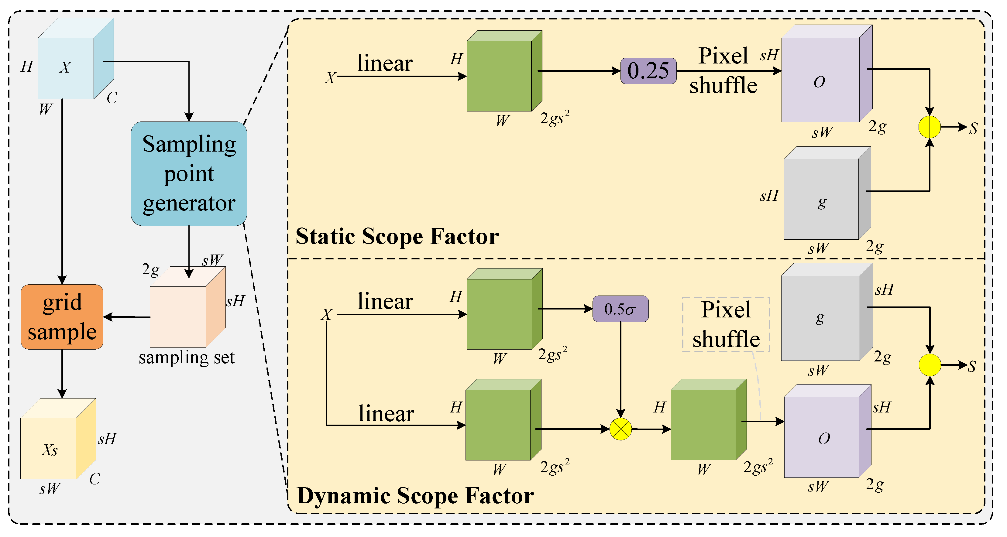
2.3.2. Neck Network Architecture and Feature Enhancement Module Co-Optimization
2.3.3. Powerful Intersection over Union v2
- (1)
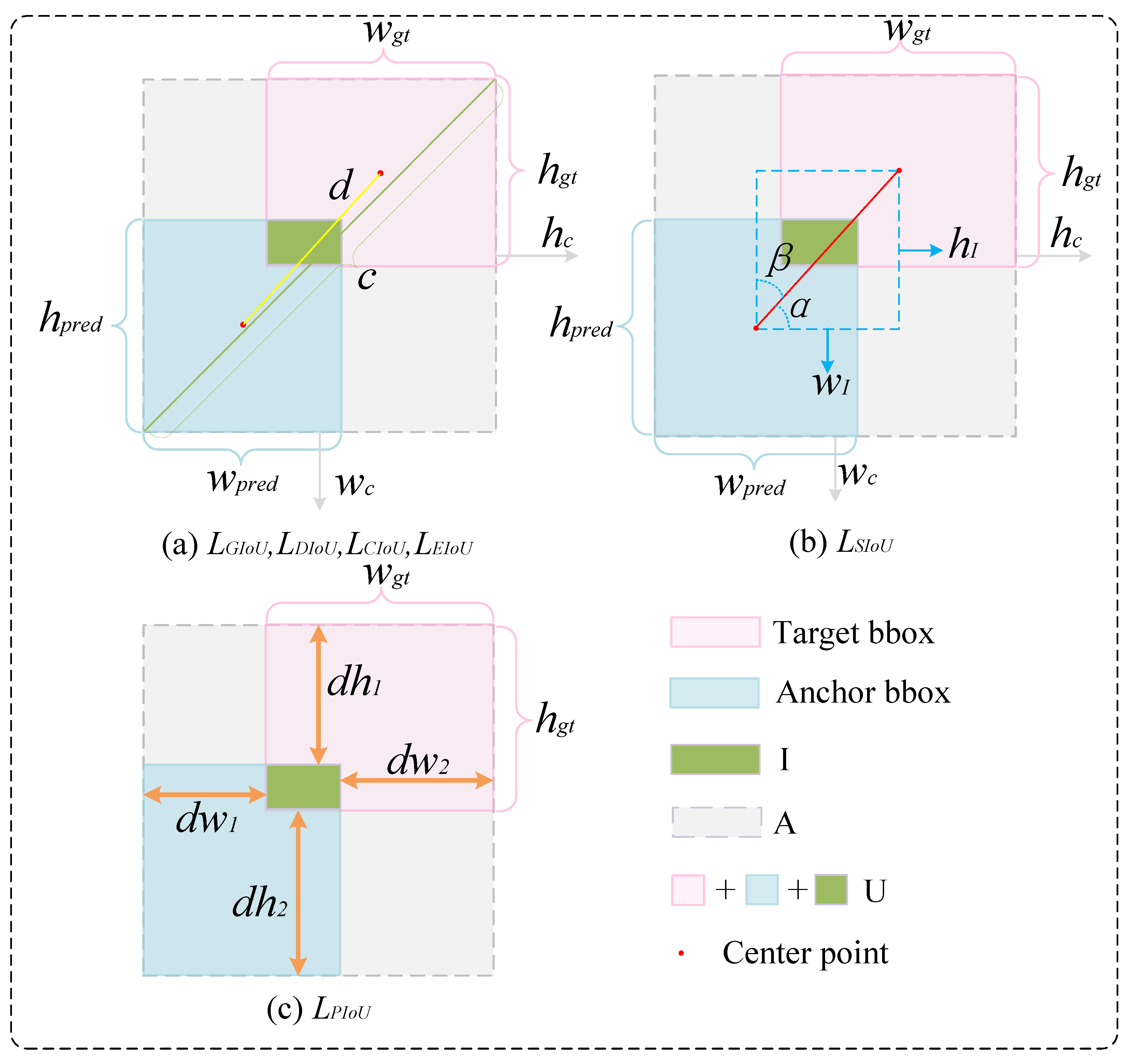
- Size -Adaptive Penalty Factorwhere and represent the absolute distances between the predicted box’s left and right edges and the corresponding edges of the ground truth box, respectively. and denote the absolute distances between the predicted box’s top and bottom edges and the corresponding edges of the ground truth box, respectively. and correspond to the width and height of the ground truth box, respectively. Notably, depends solely on the ground truth box dimensions—anchor box enlargement does not affect P—thus preventing area inflation.
- (2)
- Nonlinear Gradient Modulation FunctionIts gradient isWhen (extreme anchor boxes), is small, suppressing harmful gradients. When (moderate quality), reaches its maximum, accelerating anchor box convergence. When (high quality), decreases, stabilizing the alignment.
- (3)
- Definition of PIoU LossThe “Powerful IoU” metric is introduced:The final PIoU loss is defined aswhere and I represent the intersection areas between the predicted box and the ground truth box, while U denotes their union area. To further address the issue of imbalanced gradient contributions caused by varying training sample quality, PIoUv2 introduces a non-monotonic attention mechanism based on PIoU. This mechanism focuses primarily on medium-quality anchors while suppressing the negative impact of low-quality samples. The quality metric is defined asThe non-monotonic attention function is defined asTherefore, the final PIoUv2 loss is defined aswhere is the sole tuning hyperparameter that controls the peak position of the attention function. q represents the similarity metric between the anchor box and the target box, where a q value closer to 1 represents higher quality. The function curve of exhibits a non-monotonic shape, reaching its maximum response at intermediate values, thereby assigning the greatest optimization weight to the anchor boxes of moderate quality.
2.4. Model Training and Testing
2.4.1. Test Environment and Parameter Settings
2.4.2. Evaluation Indicators
- (1)
- Precision: Precision measures the proportion of correctly detected instances among all detected instances. It is defined as the ratio of TPs to the total number of detections. It is formulated as
- (2)
- Recall: Recall primarily evaluates the model’s ability to detect all relevant instances within the test dataset. It is defined as the ratio between the number of correctly detected instances and the total number of actual instances present. Its computation is given by
- (3)
- mAP@0.5: The mean average precision () at an IoU threshold of 0.5 represents the average of the values computed for all categories, and if the IoU between the predicted bounding box and the ground truth box is greater than or equal to 0.5, the detection is considered correct. This metric provides a comprehensive assessment of the model’s overall detection capability under a relatively lenient localization requirement. The calculation is defined aswhere N denotes the total number of categories and represents the precision for category c. The metric is obtained by integrating the precision–recall (P-R) curve, which is computed as the area under the curve: .
- (4)
- mAP@[0.5:0.95]: It refers to the mAP computed across multiple IoU thresholds ranging from 0.5 to 0.95 with a step size of 0.05. This metric comprehensively evaluates the model’s performance under varying localization precision requirements. A higher value indicates that the target object is localized more accurately. Its calculation is defined aswhere N denotes the total number of categories and represents the precision of category c at the k IoU threshold. is computed by integrating the P-R curve, namely by calculating the area under the curve: .
3. Results and Analysis
3.1. GDFC Experiments
3.2. DF-Neck Experiments
3.3. PIoUv2 Experiments
- (1)
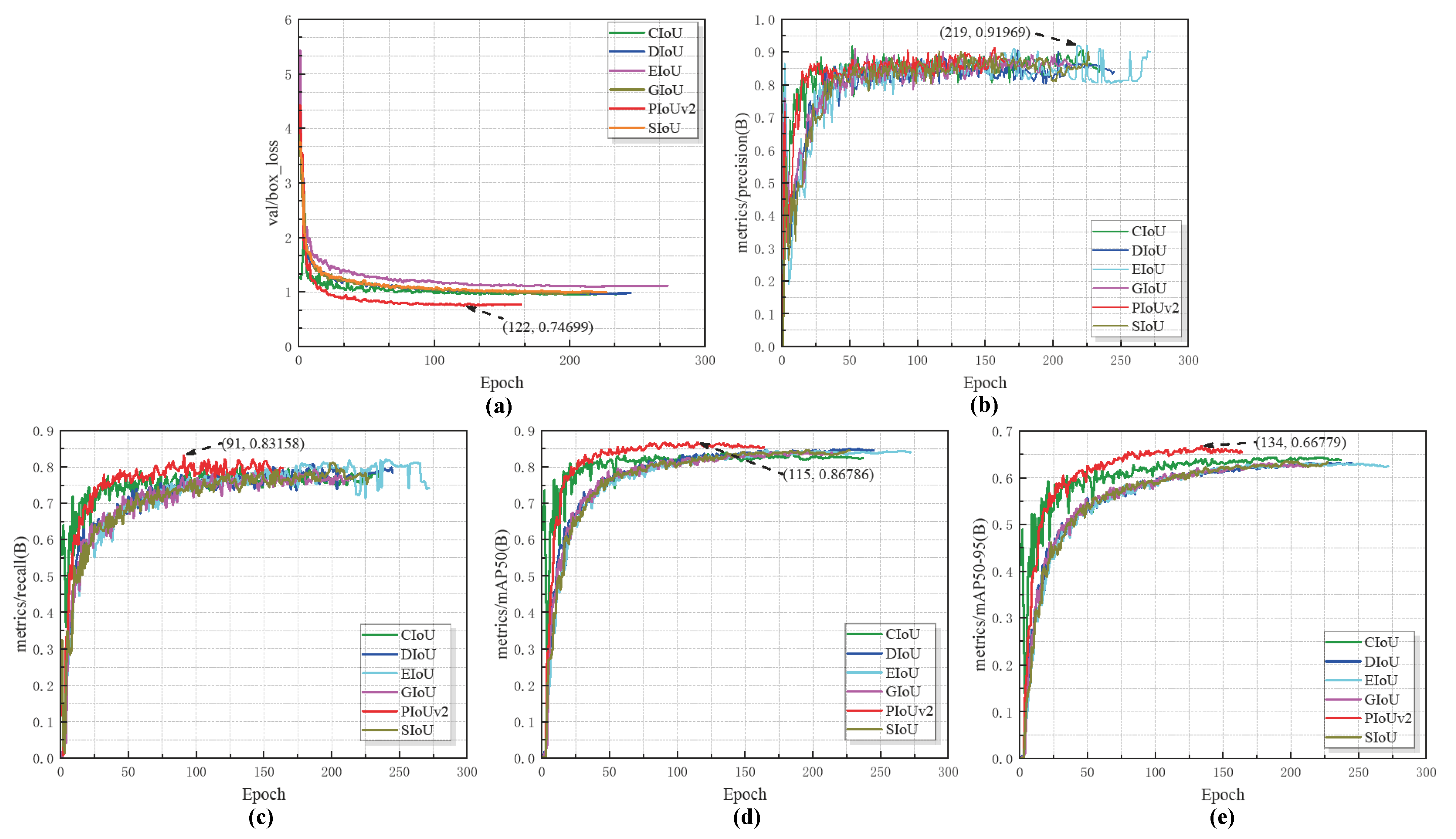
- Convergence speed analysisThe results show that for the val/box_loss metric, PIoUv2 reached its optimal value as early as epoch 122, while for the mAP@0.5 metric, PIoUv2 reached its best performance as early as epoch 115. As for the mAP@[0.5:0.95] metric, its best advantage is that it occurs at epoch 134. Also, PIoUv2 reached its peak at epoch 91. Only the precision metric is an exception. For this metric, the performance of EIoU is slightly better. It reached its best state at epoch 219. Overall, PIoUv2 shows a faster convergence speed in most indicators. It can achieve stable performance earlier than those competing loss functions, which indicates that it is superior in terms of training convergence efficiency.
- (2)
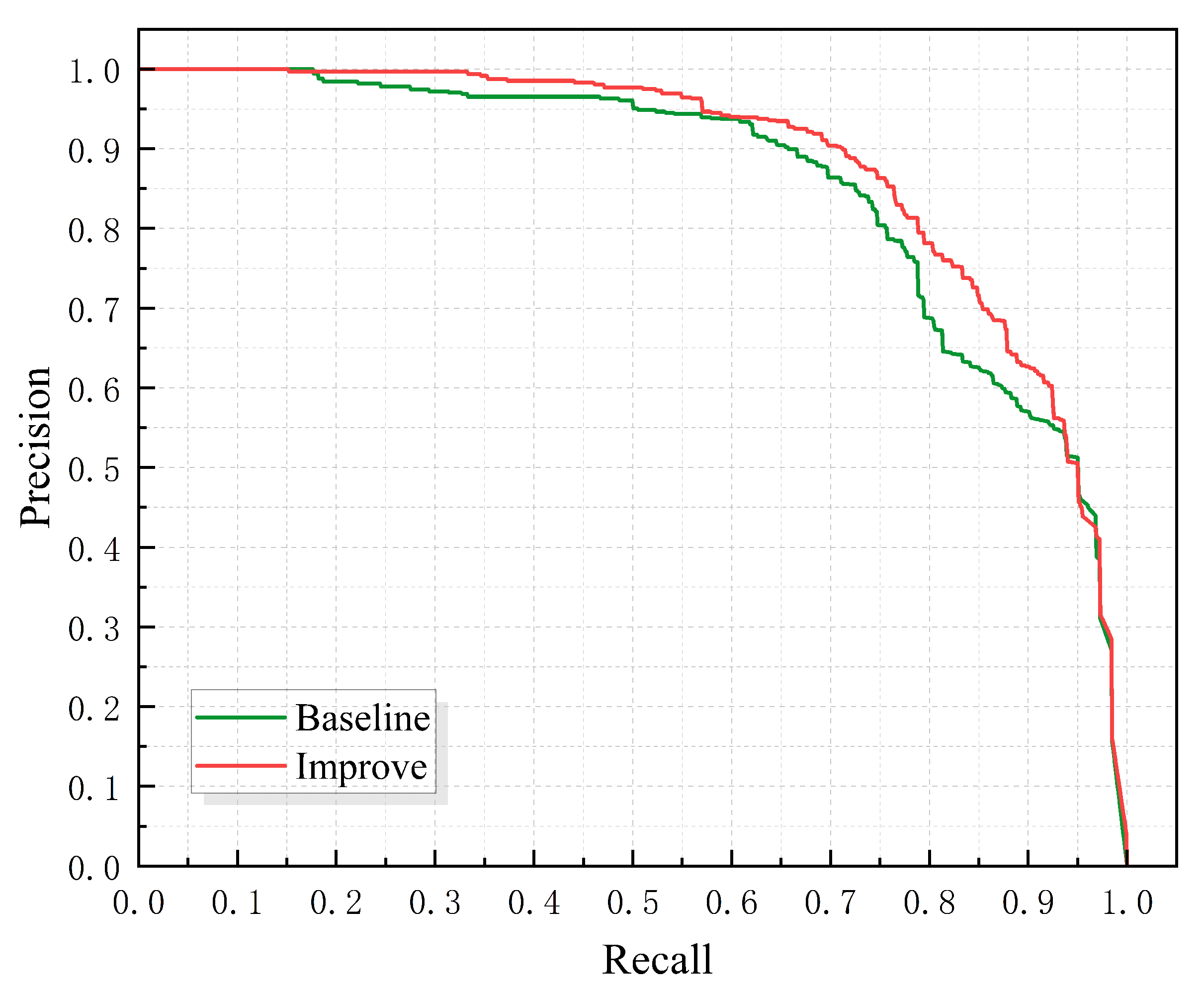
- Regression Accuracy AnalysisFrom the perspective of the final regression accuracy, PIoUv2 also demonstrates a very prominent advantage. By comparing the end-of-training metrics including mAP@0.5, mAP@[0.5:0.95], accuracy, and recall, it is easy to see that PIoUv2 performs well in key metrics such as mAP@0.5, mAP@[0.5:0.95], and recall, all achieving the highest scores. Although its accuracy is slightly lower than that of EIoU, the difference is very small. Its overall performance is still superior. During the entire training process of PIoUv2, its fluctuation is relatively small, the curve is smoother, and its regression characteristics are more stable. In order to comprehensively compare the detection accuracy of different regression loss functions, Table 5 summarizes the key metrics obtained after training each method: mAP@0.5, mAP@[0.5:0.95], precision, and recall.
3.4. Ablation Study
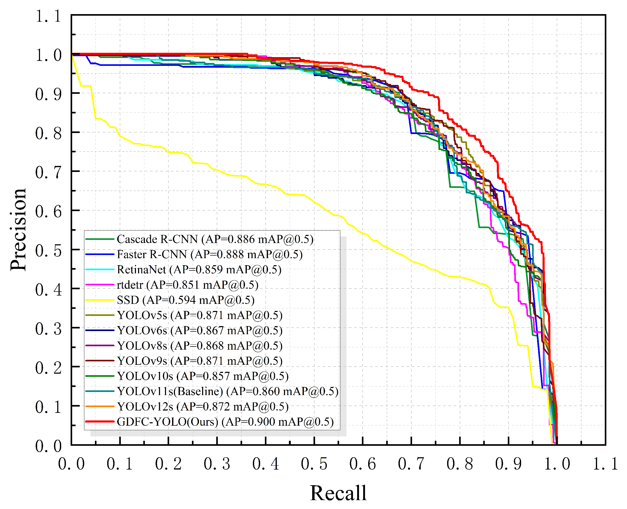
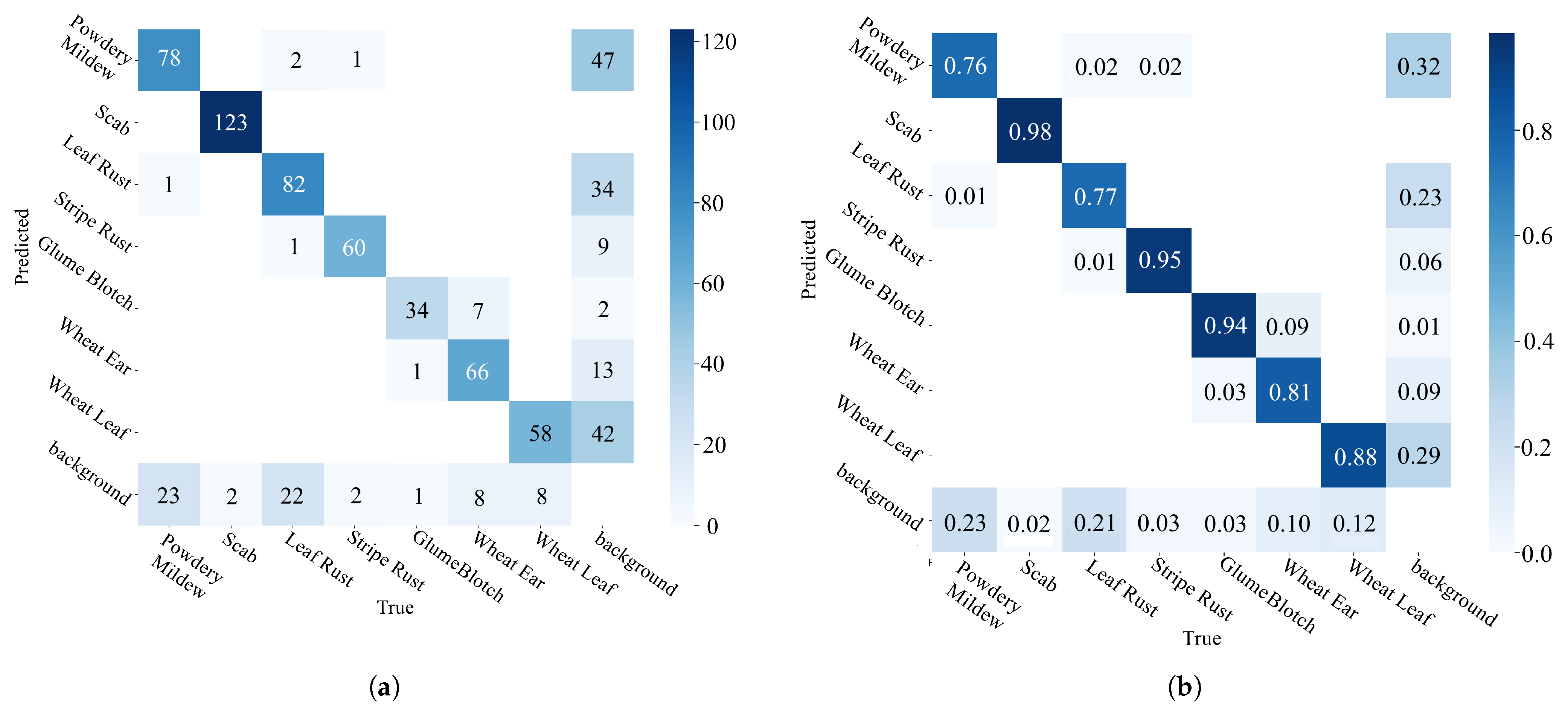
3.5. Model Comparison Experiments
3.6. Model Generalization Experiments
4. Conclusions
Author Contributions
Funding
Institutional Review Board Statement
Informed Consent Statement
Data Availability Statement
Conflicts of Interest
References
- Grote, U.; Fasse, A.; Nguyen, T.T.; Erenstein, O. Food security and the dynamics of wheat and maize value chains in Africa and Asia. Front. Sustain. Food Syst. 2021, 4, 617009. [Google Scholar] [CrossRef]
- Li, Y.; Liu, W.C.; Zhao, Z.H. The occurrence and management of wheat insect pests and diseases in China in 2022 and reflections on pest control measures. China Plant Prot. 2023, 43, 52–54. [Google Scholar]
- Ghazal, S.; Munir, A.; Qureshi, W.S. Computer vision in smart agriculture and precision farming: Techniques and applications. Artif. Intell. Agric. 2024, 13, 64–83. [Google Scholar] [CrossRef]
- Qiu, Z.; Wang, F.; Li, T.; Liu, C.; Jin, X.; Qing, S.; Shi, Y.; Wu, Y.; Liu, C. LGWheatNet: A Lightweight Wheat Spike Detection Model Based on Multi-Scale Information Fusion. Plants 2025, 14, 1098. [Google Scholar] [CrossRef] [PubMed]
- Yao, X.; Yang, F.; Yao, J. YOLO-Wheat: A Wheat Disease Detection Algorithm Improved by YOLOv8s. IEEE Access 2024, 12, 133877–133888. [Google Scholar] [CrossRef]
- Kumar, D.; Kukreja, V. CaiT-YOLOv9: Hybrid Transformer Model for Wheat Leaf Fungal Head Prediction and Diseases Classification. Int. J. Inf. Technol. 2025, 17, 2749–2763. [Google Scholar] [CrossRef]
- Zhong, D.; Wang, P.; Shen, J.; Zhang, D. Detection of Wheat Pest and Disease in Complex Backgrounds Based on Improved YOLOv8 Model. Int. J. Adv. Comput. Sci. Appl. 2025, 16, 1080. [Google Scholar] [CrossRef]
- Bao, W.; Huang, C.; Hu, G.; Su, B.; Yang, X. Detection of Fusarium Head Blight in Wheat Using UAV Remote Sensing Based on Parallel Channel Space Attention. Comput. Electron. Agric. 2024, 217, 108630. [Google Scholar] [CrossRef]
- Volety, D.R.; RamanThakur; Mishra, S.; Goel, S.; Garg, R.; Yamsani, N. Wheat Disease Detection Using YOLOv8 and GAN Model. In Innovative Computing and Communications; Springer: Singapore, 2024; pp. 349–363. [Google Scholar]
- Doroshenko, O.V.; Golub, M.V.; Kremneva, O.Y.; Shcherban’, P.S.; Peklich, A.S.; Danilov, R.Y.; Gasiyan, K.E.; Ponomarev, A.V.; Lagutin, I.N.; Moroz, I.A.; et al. Automated Assessment of Wheat Leaf Disease Spore Concentration Using a Smart Microscopy Scanning System. Agronomy 2024, 14, 1945. [Google Scholar] [CrossRef]
- Jiang, Q.; Wang, H.; Sun, Z.; Cao, S.; Wang, H. YOLOv5s-Based Image Identification of Stripe Rust and Leaf Rust on Wheat at Different Growth Stages. Plants 2024, 13, 2835. [Google Scholar] [CrossRef] [PubMed]
- Sharma, J.; Kumar, D.; Chattopadhay, S.; Kukreja, V.; Verma, A. A YOLO-Based Framework for Accurate Identification of Wheat Mosaic Virus Disease. In Proceedings of the 2024 11th International Conference on Reliability, Infocom Technologies and Optimization (Trends and Future Directions) (ICRITO), Noida, India, 14–15 March 2024; IEEE: Piscataway, NJ, USA, 2024; pp. 1–4. [Google Scholar]
- Önler, E.; Köycü, N.D. Wheat Powdery Mildew Detection with YOLOv8 Object Detection Model. Appl. Sci. 2024, 14, 7073. [Google Scholar] [CrossRef]
- Mao, R.; Zhang, Y.; Wang, Z.; Hao, X.; Zhu, T.; Gao, S.; Hu, X. DAE-Mask: A novel deep-learning-based automatic detection model for in-field wheat diseases. Precis. Agric. 2024, 25, 785–810. [Google Scholar] [CrossRef]
- Sharma, J.; Kumar, D.; Chattopadhay, S.; Kukreja, V.; Verma, A. Wheat Powdery Mildew Automatic Identification Through YOLOv8 Instance Segmentation. In Proceedings of the 2024 11th International Conference on Reliability, Infocom Technologies and Optimization (Trends and Future Directions) (ICRITO), Noida, India, 14–15 March 2024; IEEE: Piscataway, NJ, USA, 2024; pp. 1–5. [Google Scholar]
- Han, K.; Wang, Y.; Guo, J.; Wu, E. ParameterNet: Parameters Are All You Need for Large-scale Visual Pretraining of Mobile Networks. In Proceedings of the IEEE/CVF Conference on Computer Vision and Pattern Recognition (CVPR), Seattle, WA, USA, 16–22 June 2024; pp. 15751–15761. [Google Scholar]
- Si, Y.; Xu, H.; Zhu, X.; Zhang, W.; Dong, Y.; Chen, Y.; Li, H. SCSA: Exploring the synergistic effects between spatial and channel attention. Neurocomputing 2025, 634, 129866. [Google Scholar] [CrossRef]
- Liu, W.; Lu, H.; Fu, H.; Cao, Z. Learning to Upsample by Learning to Sample. In Proceedings of the IEEE/CVF International Conference on Computer Vision (ICCV), Paris, France, 1–6 October 2023; pp. 6027–6037. [Google Scholar]
- Finder, S.E.; Amoyal, R.; Treister, E.; Freifeld, O. Wavelet Convolutions for Large Receptive Fields. In Computer Vision—ECCV 2024; Leonardis, A., Ricci, E., Roth, S., Russakovsky, O., Sattler, T., Varol, G., Eds.; Lecture Notes in Computer Science; Springer: Cham, Switzerland, 2025; Volume 15112, pp. 363–380. [Google Scholar]
- Rezatofighi, H.; Tsoi, N.; Gwak, J.; Sadeghian, A.; Reid, I.; Savarese, S. Generalized Intersection Over Union: A Metric and a Loss for Bounding Box Regression. In Proceedings of the IEEE/CVF Conference on Computer Vision and Pattern Recognition (CVPR), Long Beach, CA, USA, 15–20 June 2019; pp. 658–666. [Google Scholar]
- Zheng, Z.; Wang, P.; Liu, W.; Li, J.; Ye, R.; Ren, D. Distance-IoU Loss: Faster and Better Learning for Bounding Box Regression. In Proceedings of the AAAI Conference on Artificial Intelligence, New York, NY, USA, 7–12 February 2020; pp. 12993–13000. [Google Scholar]
- Zhang, Y.-F.; Ren, W.; Zhang, Z.; Jia, Z.; Wang, L.; Tan, T. Focal and efficient IOU loss for accurate bounding box regression. Neurocomputing 2022, 506, 146–157. [Google Scholar] [CrossRef]
- Gevorgyan, Z. SIoU loss: More powerful learning for bounding box regression. arXiv 2022, arXiv:2205.12740. [Google Scholar] [CrossRef]
- Liu, C.; Wang, K.; Li, Q.; Zhao, F.; Zhao, K.; Ma, H. Powerful-IoU: More straightforward and faster bounding box regression loss with a nonmonotonic focusing mechanism. Neural Netw. 2024, 170, 276–284. [Google Scholar] [CrossRef] [PubMed]
- Gao, C.; Guo, W.; Yang, C.; Gong, Z.; Yue, J.; Fu, Y.; Feng, H. A fast and lightweight detection model for wheat fusarium head blight spikes in natural environments. Comput. Electron. Agric. 2024, 216, 108484. [Google Scholar] [CrossRef]
- Singh, D.; Jain, N.; Jain, P.; Kayal, P.; Kumawat, S.; Batra, N. PlantDoc: A Dataset for Visual Plant Disease Detection. In Proceedings of the 7th ACM IKDD CoDS and 25th COMAD, Hyderabad, India, 5–7 January 2020; pp. 249–253. [Google Scholar]
- Hughes, D.; Salathé, M. An open access repository of images on plant health to enable the development of mobile disease diagnostics. arXiv 2015, arXiv:1511.08060. [Google Scholar]

| Disease Category | Training Set | Validation Set | Test Set | Total Instances | Category Proportion |
|---|---|---|---|---|---|
| Powdery Mildew | 810 | 102 | 108 | 1020 | 17.45% |
| Scab | 1060 | 125 | 110 | 1295 | 22.16% |
| Leaf Rust | 827 | 107 | 102 | 1036 | 17.73% |
| Stripe Rust | 470 | 63 | 60 | 593 | 10.15% |
| Glume Blotch | 351 | 36 | 41 | 428 | 7.32% |
| Wheat Ear | 491 | 81 | 52 | 624 | 10.68% |
| Wheat Leaf | 680 | 66 | 103 | 849 | 14.53% |
| Total | 4689 | 580 | 576 | 5845 | 100% |
| Model | GFLOPs | Params (M) | Model File Size | FPS | mAP@0.5 |
|---|---|---|---|---|---|
| Bsaeline | 21.6 | 9.43 | 18.3 MB | 150.7 | 0.860 |
| GDFC (N = 1) | 19.9 | 8.89 | 17.5 MB | 68.79 | 0.886 |
| GDFC (N = 2) | 20.9 | 9.48 | 36.8 MB | 45.46 | 0.897 |
| GDFC (N = 3) | 21.9 | 10.07 | 39.2 MB | 33.73 | 0.887 |
| Model | P | R | mAP@0.5 | mAP@[0.5:0.95] |
|---|---|---|---|---|
| Bsaeline | 0.853 | 0.825 | 0.860 | 0.681 |
| GDFC | 0.888 | 0.819 | 0.886 | 0.696 |
| Model | P | R | mAP@0.5 | mAP@[0.5:0.95] |
|---|---|---|---|---|
| Bsaeline | 0.853 | 0.825 | 0.860 | 0.681 |
| DF-Neck | 0.891 | 0.816 | 0.886 | 0.672 |
| Experiments | P | R | mAP@0.5 | mAP@[0.5:0.95] |
|---|---|---|---|---|
| CIoU | 0.853 | 0.825 | 0.860 | 0.681 |
| EIoU | 0.923 | 0.793 | 0.866 | 0.667 |
| SIoU | 0.901 | 0.792 | 0.868 | 0.675 |
| DIoU | 0.878 | 0.815 | 0.876 | 0.674 |
| GIoU | 0.885 | 0.801 | 0.869 | 0.677 |
| PIoUv2 | 0.916 | 0.805 | 0.885 | 0.692 |
| Baseline | GDFC | DF-Neck | PIoUv2 | P | R | mAP@0.5 | mAP@ [0.5:0.95] | Params (M) | GFLOPs |
|---|---|---|---|---|---|---|---|---|---|
| ✓ | 0.853 | 0.825 | 0.860 | 0.681 | 9.43 | 21.6 | |||
| ✓ | ✓ | 0.888 | 0.819 | 0.886 | 0.696 | 8.89 | 19.9 | ||
| ✓ | ✓ | 0.891 | 0.816 | 0.886 | 0.672 | 9.81 | 24.3 | ||
| ✓ | ✓ | 0.916 | 0.805 | 0.885 | 0.692 | 9.43 | 21.6 | ||
| ✓ | ✓ | ✓ | 0.872 | 0.829 | 0.894 | 0.691 | 9.27 | 22.5 | |
| ✓ | ✓ | ✓ | 0.870 | 0.835 | 0.889 | 0.693 | 8.89 | 19.9 | |
| ✓ | ✓ | ✓ | 0.893 | 0.813 | 0.889 | 0.697 | 9.81 | 24.3 | |
| ✓ | ✓ | ✓ | ✓ | 0.899 | 0.821 | 0.900 | 0.695 | 9.27 | 22.5 |
| Method | P | R | mAP@0.5 | mAP@[0.5:0.95] | Params (M) | GFLOPs |
|---|---|---|---|---|---|---|
| rtdetr | 0.871 | 0.798 | 0.851 | 0.645 | 42.78 | 130.5 |
| Cascade R-CNN | 0.889 | 0.835 | 0.886 | 0.711 | 69.17 | 99.4 |
| Faster R-CNN | 0.882 | 0.843 | 0.888 | 0.710 | 41.38 | 71.6 |
| RetinaNet | 0.865 | 0.815 | 0.859 | 0.652 | 19.90 | 46.8 |
| SSD | 0.597 | 0.651 | 0.594 | 0.341 | 24.55 | 105.5 |
| YOLOv12s | 0.919 | 0.780 | 0.872 | 0.669 | 9.10 | 19.6 |
| YOLOv11s | 0.853 | 0.825 | 0.860 | 0.681 | 9.43 | 21.6 |
| YOLOv10s | 0.895 | 0.785 | 0.857 | 0.671 | 8.07 | 24.8 |
| YOLOv9s | 0.911 | 0.797 | 0.871 | 0.667 | 6.32 | 22.7 |
| YOLOv8s | 0.894 | 0.789 | 0.868 | 0.664 | 9.84 | 23.6 |
| YOLOv6s | 0.887 | 0.799 | 0.867 | 0.667 | 15.99 | 43.0 |
| YOLOv5s | 0.889 | 0.806 | 0.871 | 0.677 | 7.83 | 19.0 |
| Ours | 0.899 | 0.821 | 0.900 | 0.695 | 9.27 | 22.5 |
| Dataset | P | R | mAP@0.5 | mAP@[0.5:0.95] | Params (M) | GFLOPs |
|---|---|---|---|---|---|---|
| Plant-Village | 0.854 | 0.832 | 0.916 | 0.902 | 9.28 | 22.6 |
| PlantDoc | 0.874 | 0.811 | 0.918 | 0.719 | 9.28 | 22.6 |
| LWDCD 2020 | 0.891 | 0.845 | 0.92 | 0.631 | 9.27 | 22.5 |
Disclaimer/Publisher’s Note: The statements, opinions and data contained in all publications are solely those of the individual author(s) and contributor(s) and not of MDPI and/or the editor(s). MDPI and/or the editor(s) disclaim responsibility for any injury to people or property resulting from any ideas, methods, instructions or products referred to in the content. |
© 2025 by the authors. Licensee MDPI, Basel, Switzerland. This article is an open access article distributed under the terms and conditions of the Creative Commons Attribution (CC BY) license (https://creativecommons.org/licenses/by/4.0/).
Share and Cite
Qian, J.; Dai, C.; Ji, Z.; Liu, J. GDFC-YOLO: An Efficient Perception Detection Model for Precise Wheat Disease Recognition. Agriculture 2025, 15, 1526. https://doi.org/10.3390/agriculture15141526
Qian J, Dai C, Ji Z, Liu J. GDFC-YOLO: An Efficient Perception Detection Model for Precise Wheat Disease Recognition. Agriculture. 2025; 15(14):1526. https://doi.org/10.3390/agriculture15141526
Chicago/Turabian StyleQian, Jiawei, Chenxu Dai, Zhanlin Ji, and Jinyun Liu. 2025. "GDFC-YOLO: An Efficient Perception Detection Model for Precise Wheat Disease Recognition" Agriculture 15, no. 14: 1526. https://doi.org/10.3390/agriculture15141526
APA StyleQian, J., Dai, C., Ji, Z., & Liu, J. (2025). GDFC-YOLO: An Efficient Perception Detection Model for Precise Wheat Disease Recognition. Agriculture, 15(14), 1526. https://doi.org/10.3390/agriculture15141526