Article

Assessing Methane Emissions from Rice Fields in Large Irrigation Projects Using Satellite-Derived Land Surface Temperature and Agronomic Flooding: A Spatial Analysis

by
Sellaperumal Pazhanivelan
1,*,
N. S. Sudarmanian
2,
Vellingiri Geethalakshmi
1,
Murugesan Deiveegan
3,
Kaliaperumal Ragunath
1,
A. P. Sivamurugan
1 and
P. Shanmugapriya
1
1
Centre for Water and Geospatial Studies, Tamil Nadu Agricultural University, Coimbatore 641003, India
2
Department of Remote Sensing and GIS, Tamil Nadu Agricultural University, Coimbatore 641003, India
3
International Rice Research Institute, South Asia Regional Centre, Varanasi 221106, India
*
Author to whom correspondence should be addressed.
Agriculture 2024, 14(3), 496; https://doi.org/10.3390/agriculture14030496
Submission received: 10 January 2024 / Revised: 7 March 2024 / Accepted: 12 March 2024 / Published: 19 March 2024

Abstract

:
Synthetic aperture radar (SAR) imagery, notably Sentinel-1A’s C-band, VV, and VH polarized SAR, has emerged as a crucial tool for mapping rice fields, especially in regions where cloud cover hinders optical imagery. Employing multi-temporal characteristics, SAR data were regularly collected and parameterized using MAPscape-Rice software, which integrates a fully automated processing chain to convert the data into terrain-geocoded σ° values. This facilitated the generation of rice area maps through a rule-based classifier approach, with classification accuracies ranging from 88.5 to 91.5 and 87.5 percent in 2017, 2018, and 2022, respectively. To estimate methane emissions, IPCC (37.13 kg/ha/season, 42.10 kg/ha/season, 43.19 kg/ha/season) and LST (36.05 kg/ha/season, 41.44 kg/ha/season, 38.07 kg/ha/season) factors were utilized in 2017, 2018 and 2022. Total methane emissions were recorded as 19.813 Gg, 20.661 Gg, and 25.72 Gg using IPCC and 19.155 Gg, 20.373 Gg, and 22.76 Gg using LST factors in 2017, 2018 and 2022. Overall accuracy in methane emission estimation, assessed against field observations, ranged from (IPCC) 85.71, 91.32, and 80.25 percent to (LST) 83.69, 91.43, and 84.69 percent for the years 2017, 2018 and 2022, respectively, confirming the efficacy of remote sensing in greenhouse gas monitoring and its potential for evaluating the impact of large-scale water management strategies on methane emissions and carbon credit-based ecosystem services at regional or national levels.

1. Introduction

Rice is the most important staple food, feeding millions of people more than any other crop and farmed on millions of hectares across South and Southeast Asian countries. Unlike other crops, rice can grow in damp conditions, making it distinct. However, because of the anaerobic condition in which it is grown, the crop contributes to global warming by emitting methane into the atmosphere. It has long been known that methane emissions from paddy fields contribute significantly to greenhouse gas emissions from anthropogenic sources [1]. Its emission from rice fields is caused by a unique ecosystem dominated by microbial-mediated anaerobic activity compared to that of natural wetlands but integrating agronomic practices of irrigation and fertilizer use. The cultivation systems, viz., irrigated, semidry, rainfed and deep-water systems, largely influence methane emission. Further, these emissions vary with the cultivars and nature of inputs, viz., nitrogenous fertilizers and application of organic manures [2]. An unprecedented increase in the global rice area by 40 percent in the last 50 years [3]. Methane (CH4) is a significant greenhouse gas (GHG) among all the components of the atmosphere. Based on 100-year global warming potentials, the Inter-governmental Panel on Climate Change (IPCC) estimates that the warming forces of CH4 are 25 to 30 times greater than those of CO2 per unit of weight [4].
Methane emissions are expected to rise shortly due to rice fields in South and Southeast Asia [5] contributing to roughly 10–15 percent of worldwide CH4 emissions [6], with an estimated yearly emission of 50–100 Tg of methane. This means that an increase in rice production will result in a 36 percent rise in methane emissions from these fields [7]. Rice fields that have been flooded are the third greatest agricultural source of emissions, accounting for between 10 and 30 percent of the methane produced worldwide by the anaerobic breakdown of organic waste [8]. On the contrary, upland paddy, which is not flooded and does not release greenhouse gases into the atmosphere, makes up around 15 percent of the 150 Mha worldwide paddy harvest area. An area of approximately 127 Mha is made up of other paddy fields with rainfed, deep water and irrigated water regimes; over 90 percent of these are in Asia [9,10], with the maximum extent in India (42.2 Mha).
Hence, it is crucial to understand the mechanism and spatiotemporal patterns of global and regional methane emission from rice fields. Global level estimation and monitoring of methane emission are performed widely to understand its contribution to greenhouse gases and develop management strategies. Therefore, several nations worldwide, including China, India, Indonesia, Thailand, and the Philippines, have already started initiatives to estimate country-specific contributions to the global methane emissions from paddy fields. These initiatives are coordinated by the International Rice Research Institute (IRRI). The emission rate may differ within a country or the same rice fields, depending on the estimation methods used. Based on the recommendations from earlier research [10,11], the methane emissions from irrigated rice fields in key rice-producing nations such as China, India, Bangladesh, Indonesia, and Thailand were calculated to be 7.41, 3.99, 0.47, 1.28, and 0.18 Tg yearly, respectively [12].
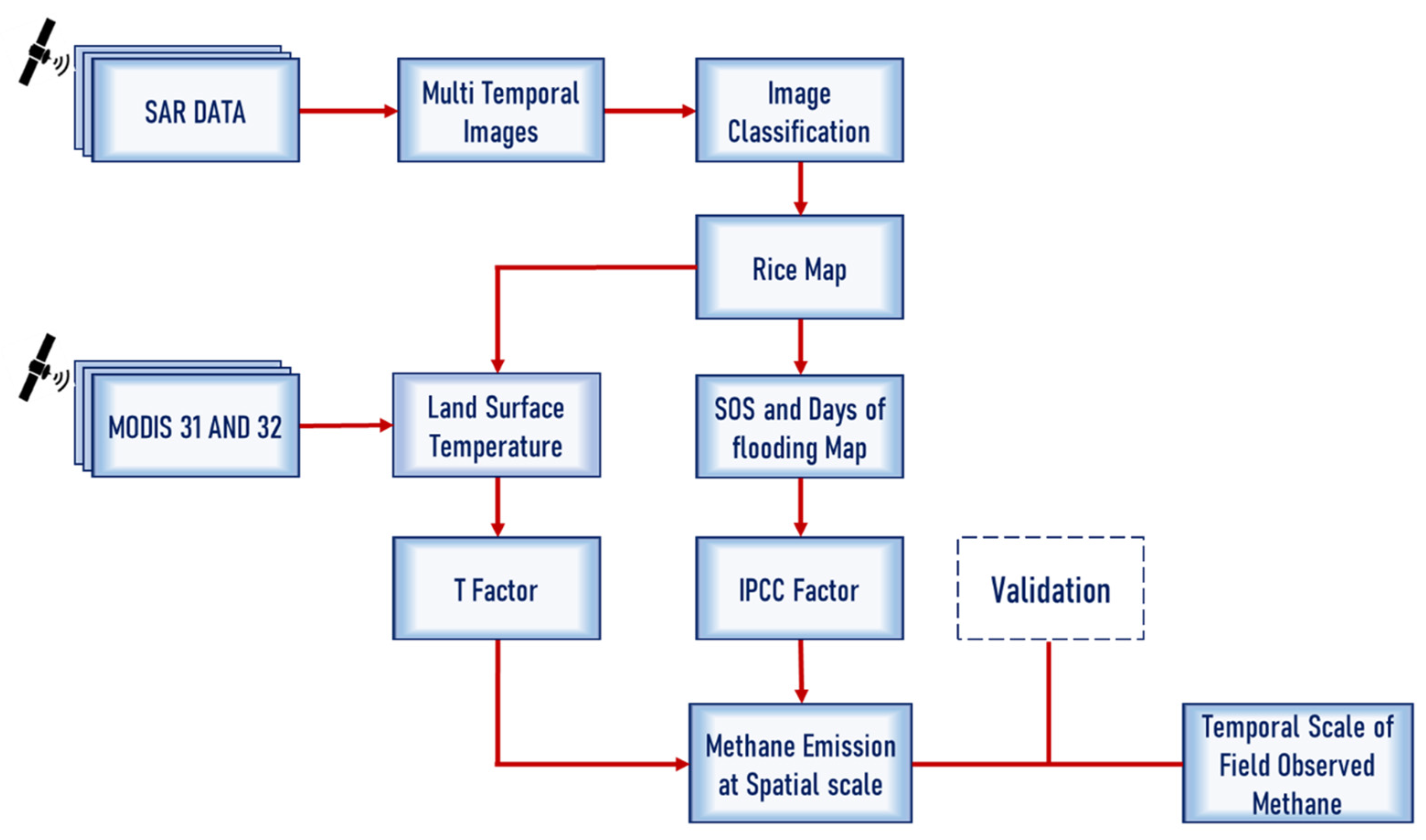
Conventional methods for estimating methane emissions for larger areas are tedious, time-consuming and laborious and have become impractical. These constraints warranted the use of more scientific methods through remote sensing. Remote sensing provides the scope to be used as a tool to detect and quantify methane emission with recent advances in SAR sensors capable of providing accurate estimates in rice areas, seasonality and days of flooding. The emissions from the irrigated rice fields in China, India, Indonesia, the Philippines, and Thailand were estimated using Geographic Information System (GIS) tools and models. In addition to the spatial connection of land surface temperature, precise estimation of methane emission from rice fields at a regional scale depends on an exact evaluation of the rice acreage and the associated period of flooding in those fields. Land surface temperature (LST) has been used as one of the important parameters for the estimation of emitted methane. Land surface temperature (LST) provides a better indication of energy balance and the greenhouse effect on the earth’s surface and plays a vital role in the physics of land surface processes on a global scale. LST can be derived from MODIS land products and used to assess the rate of methane emission from rice fields through different algorithms [13]. Cloud cover presents a problem in mapping and monitoring the flooded condition of rice crops. However, there are sustainable solutions available owing to the recent and upcoming deployments of synthetic aperture radar (SAR) sensors and advanced automated processing. Therefore, it is now possible to estimate methane emissions from rice fields spatially to create a greenhouse gas inventory which helps in recommending mitigation strategies at the regional level.
Considering these aspects, the following goals guided the conduct of this research: Quantification of CH4 emissions from rice fields using remote sensing and GIS techniques assimilated with standard integrated flux; assessing CH4 emissions over rice fields using remote sensing-derived land surface temperature; derivation of spatial maps of CH4 emissions from the rice area at regional scale and assessing accuracy.

2. Materials and Methods

2.1. Study Area

The present investigation was carried out in Cauvery Delta Zone (CDZ) of Tamil Nadu, comprising Ariyalur, Cuddalore, Nagapattinam, Thanjavur, Thiruvarur and Tiruchirappalli districts during 2017–2018, and seven districts of Tamil Nadu viz., Mayiladuthurai, Nagapattinam, Thanjavur, Thiruvarur, Sivagangai, Ramanathapuram and Pudukkottai districts (Figure 1) during 2022. The study areas geographically lie between 78°15′ and 79°45′ East longitudes and 10°00′ and 11°30′ North latitudes, with an altitude of 90 m. The study areas were continuously monitored throughout the cropping period (Figure 2).

2.2. Data Used

The European Space Agency (ESA) and the European Commission (EC) together initiated the Sentinel-1 mission. The advantage of synthetic aperture radar (SAR) is that it can collect data in any weather, day or night, even when clouds are present. Sentinel 1A can provide consistent, dependable wide-area monitoring due to its C-SAR equipment. For land monitoring, Sentinel 1A SAR data with vertical–vertical (VV) and vertical–horizontal (VH) polarization were acquired at 12-day intervals. Sentinel 1A features four standard operating modes that are intended to facilitate system interoperability. The Level 1 ground range (GRD) product with a temporal resolution of 12 days and a resolution of 20 m was acquired using the interferometric wide (IW) sweep mode.

2.2.1. Basic Processing of SAR Data

Terrain-geocoded σ° values were obtained from SAR GRD multi-temporal data using a fully automated processing chain [14]. The MAPscape-RICE 5.6.2 software contains a module specific to the processing chain. The following steps are included in the basic processing: (i) strip mosaicking is used to facilitate overall data processing and easier handling; (ii) co-registration is used to co-register images acquired with the same observation geometry in slant range geometry; (iii) time-series speckle filtering is used to balance reflectivity differences between images; (iv) terrain geocoding is used to radiometrically calibrate and normalize images; (v) anisotropic non-linear diffusion (ANLD) filtering is used to obtain smoothed homogeneous targets; (vi) atmospheric attenuation is removed using an interpolator, and (vii) subsetting is used to shorten the processing time for raster data (Figure 3).

2.2.2. Retrieving Rice Area Using Multi-Temporal σ° Rule-Based Rice Detection

A rule-based rice detection technique was used for the multi-temporal stack of terrain-geocoded σ° images in MAPscape-RICE 5.6.2. Based on field data and knowledge of the study area, an agronomic approach was used to assess the temporal evolution of σ°. This needed prior knowledge of rice maturity, calendar and duration, as well as crop methods. The crop establishment method and crop maturity were significant factors influencing the temporal signature, which was dependent on both frequency and polarization. This suggested that while broad guidelines might be used to identify rice, the criteria for these guidelines would need to be modified by the agro-ecological zone, planting practices and rice calendar (Figure 4).

2.2.3. Use of Temporal Features to Guide Parameter Selection for the Rule-Based Classifier

A basic statistical study of the temporal signature of σ° values in the monitored fields served as the basis for the selection of parameters a, b, c, d, e and f. For every field under observation, the temporal signature’s mean, minimum, maximum and range were calculated. Then, we calculated the following: (i) the minimum and (ii) the maximum of those mean σ° values across fields; (iii) the maxima of the minimum σ° values across fields; and (iv) the minimum and (vi) maximum of the range of σ° values across fields [14]. These six statistics, which we refer to as temporal features, each directly relate to a single parameter and succinctly describe the important information in the rice signatures of the observed fields. Therefore, as seen in Table 1, the values of the six temporal features from the monitoring sites at each site can be used to inform the selection of the six parameter values.
It is easier to estimate the parameters tminlength, tmaxlength, and t2 − t1. Tminlength limits the number of days between a start-of-season detection and the subsequent highest σ° value in the temporal signature; since X-band σ° saturates before rice flowering, this value can be set to 40–70 days. Tmaxlength limits the duration between two σ° minima in the series; 120 days is a suitable cut-off representing an intensive triple-rice system (three crops in a single year). t2 − t1 is the maximum duration of agronomic flooding at the beginning of the season; this can be set to a relatively high value of 40–50 to capture even the longest land preparation phases.

2.3. Ground Truth Data Collection

Twenty rice fields in each of the research area’s districts were the locations of field observations conducted over the season. With the farmers’ permission, these fields were chosen before the scheduled image acquisition time and the start of the rice season. Ground truth and methane gas were collected from the rice fields in the same week, with respective acquisition dates. The date of image acquisition, or as close to it as possible, was used for observations. Handheld GPS receivers were used to record latitude and longitude, along with field status descriptions and images, plant height, water depth, crop stage, weather and leaf area index (LAI). Only visits between the seedling and flowering stages were used to measure LAI, which was recorded non-destructively using a smartphone application called Pocket LAI [15]. To gather data on the rice variety, source of water, crop management and cultivation techniques, as well as inputs like fertilizer and pesticide, the farmer was interviewed at the end of the growing season.
To evaluate the precision of the rice classification, a validation procedure was carried out for every image. To gather data on land cover between non-rice and rice sites, a random stratified sampling approach was used. Before harvesting, in-season surveys to validate the map were carried out throughout the reproductive or ripening phase. For 20 m resolution imagery, the locations were selected such that the land cover was uniform within a 50 m radius of each GPS point.
The mean daily methane emission rate for each field was determined by taking gas samples in the main rice-growing districts of the monitoring fields. The Agro Climate Research Centre, Tamil Nadu Agricultural University, Coimbatore, has a Shimadzu GC-2014 gas chromatograph with FID that was used to estimate the amount of methane. Using 1 ppm, 2.3 ppm and 5 ppm standards (Chemtron® Science Laboratories Pvt. Ltd., Mumbai, India) as the principal standard curve linear over the concentration ranges employed, the GC was calibrated both before and after each set of observations. The CH4 flux was calculated using Equation (1) and represented as mg m−2 h−1 [16]. Based on the equation to estimate methane emission, flux was computed, and the obtained CH4 concentrations were estimated by peak area [17].
f = (V/A) × (ΔC/Δt)
where
 
f—rate of greenhouse gas emission (mg m−2 h−1)
 
V—volume of the chamber above soil (m3)
 
A—cross-section of chamber (m2)
 
ΔC—concentration difference between zero and t times (mg cm−3)
 
Δt—time duration between two sampling periods (h)

2.4. Rice Map Accuracy Assessment

The rice/non-rice validation points collected at each site were subjected to a standard confusion matrix. It was noted how accurate the kappa value and the rice/non-rice classification were overall. The categorized rice map was evaluated for correctness by comparing it with ground truth data. The rice maps had a spatial resolution of 3 to 15 m. Nonetheless, through edge detection and locally adaptive smoothing, the ANLD filtering procedures lowered the effective resolution. The validation data were collected in areas with homogeneous land cover in a 15 m radius around each GPS point for sites using 3 m resolution imagery and a 50 m radius for sites using 10 m or 15 m resolution imagery. This was done to account for the lower resolution and the handheld GPS units’ horizontal accuracy when compared to the pixel size. The mode value of the rice map pixels within a window that matched the radius utilized in the validation land cover assessment was compared to the observed land cover at the GPS validation locations.

Kappa Coefficient

The kappa coefficient, which quantified the classifier’s proportionate (or percentage) increase over a completely random assignment to classes, was another way to assess classification accuracy [18]. The following formula was used to estimate the kappa coefficient.
K ^ = NA - B N 2 - B
If there are r rows in an error matrix, then there are also r columns,
 
where
 
A = the sum of r diagonal elements, which is the numerator in the computation of overall accuracy
 
B = sum of the r products (row total × column total)
 
N = the number of pixels in the error matrix (the sum of all r individual cell values)

2.5. Estimation of Methane Emission

2.5.1. Land Surface Temperature (LST)

An empirical model was used to estimate methane emissions. A temperature-dependent methanogenic activity model was created using the T factor (temperature-related factor). Experiments showed that the optimal temperature for most methanogens ranged from 30 °C to 40 °C [19]. Methane emission from wetlands is described by the following equation:
ECH4 = Eobs × Ft × A
where
 
Eobs is the observed methane flux from different classes,
 
Ft is the T factor,
 
A is area
 
T factor is defined as follows [19]:
F t = F ( Ts ) / F ( Ts )
where
F ( Ts ) =   e 0.334 ( Ts - 23 ) 1 + e 0.334 ( Ts - 23 )
The temperature, expressed in degrees Celsius (Ts), was determined for each pixel in the equation above using the constant emissivity approach. F ( Ts ) is the mean of F(Ts) over land. The coefficients of this exponential equation were taken from Liu [19]. Methane emission-causing classes were categorized hierarchically using the NDVI layer and the optical bands of MODIS data (1, 2, and 3). Class statistics were then obtained for each of the four classes using the categorized image and the F1 image. Data analysis and methane estimation were performed using a semi-automated process.

2.5.2. IPCC Tier 1 Method

To estimate methane emissions from rice fields, we used the IPCC Tier 1 technique (Figure 5) described in the 2006 IPCC Guidelines for National Greenhouse Gas Inventories. To calculate methane emission scaling factors, our method made use of secondary data sources along with details on rice cultural type and crop calendar. By multiplying the emission factor by the area under cultivation and the duration of the cropping period, we were able to determine the methane emission rate for each type of rice field. Next, taking into account the rice area and crop duration of each cultural type, we projected these values across the country. A standard emission factor for a range of sources, circumstances, countries, and areas is provided by the Tier 1 technique. In Tamil Nadu, the default emission factor for rice cultivation is 11 g m−2, sourced from the IPCC Emission Factor Database 2006. Under some circumstances, this emission factor can be used in rice fields for the Tier 1 technique:
CH4 rice = Σ EF × T × A × 10−6
where
 
CH4 rice = annual CH4 emission from rice cultivation in a region or country (GgCH4 a−1)
 
EF = Daily emission factor
 
T = Cultivation period
 
A = Annual harvested area of rice
To create a geoprocessing model using ArcGIS 10.8, the model was designed to analyze emissions from rice crops by considering factors such as cultivation periods, start of the season (SoS), end of the season (EOS) maps, and harvested area. This analysis was conducted at different temporal resolutions to determine the minimum and maximum emissions at various points during the growing season. After completing the analysis, an accuracy assessment was performed by collecting field samples of methane in the study area. The methane emission rate was estimated per day m−2 using gas chromatography and calculated for the entire crop growing season.

3. Experimental Results

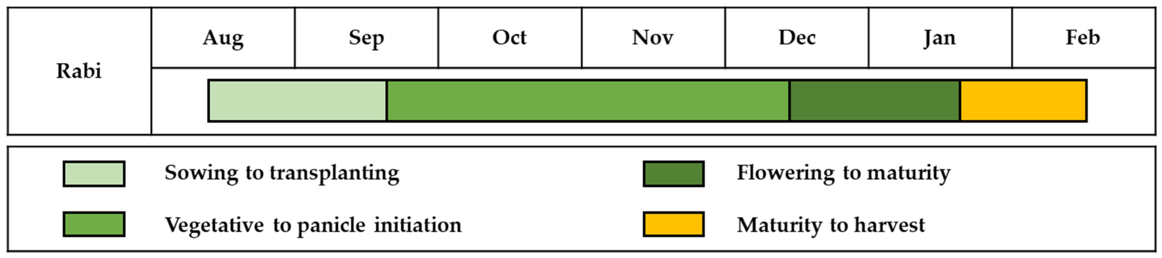
Rice is cultivated in India under irrigated and rainfed lowland conditions. The duration of most rice varieties ranges from 90 to 150 days, with three crop stages: vegetative, reproductive and maturity. The research effort was taken to map rice areas using multi-temporal C band SAR data from Sentinel 1A coupled with state-of-the-art semi-automated processing chains, in-season field monitoring and end-of-season validation points across the study area of Tamil Nadu. SAR can detect rice crops and track their growth through σo values (backscatter coefficient). Many researchers have shown interest in better understanding the relationship between backscatter and crop growth and applying them to detect rice and monitor crop growth [20,21,22,23,24,25,26].

3.1. Radar Backscattering Signature

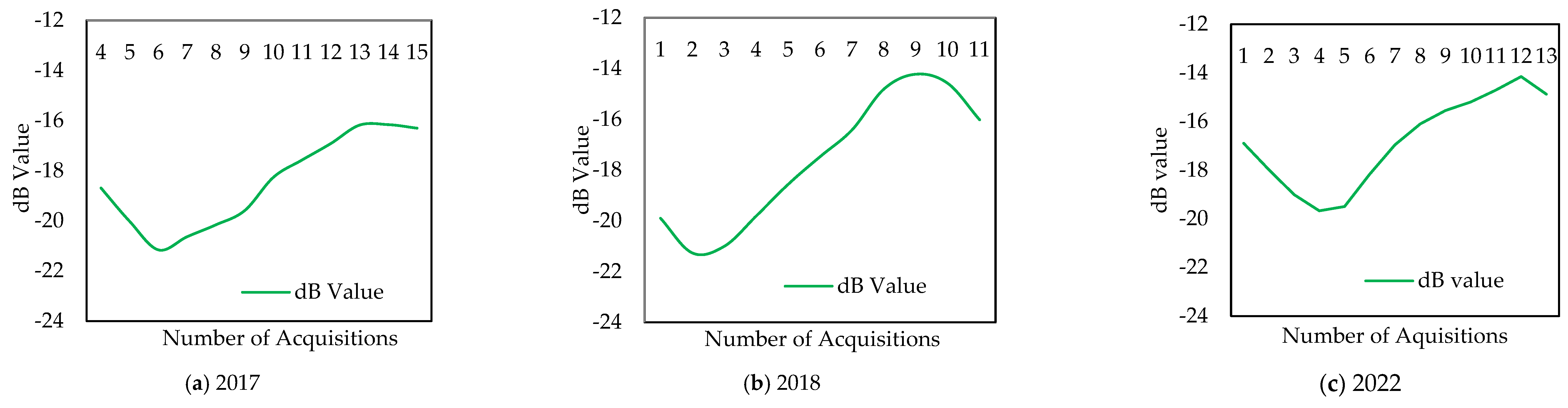
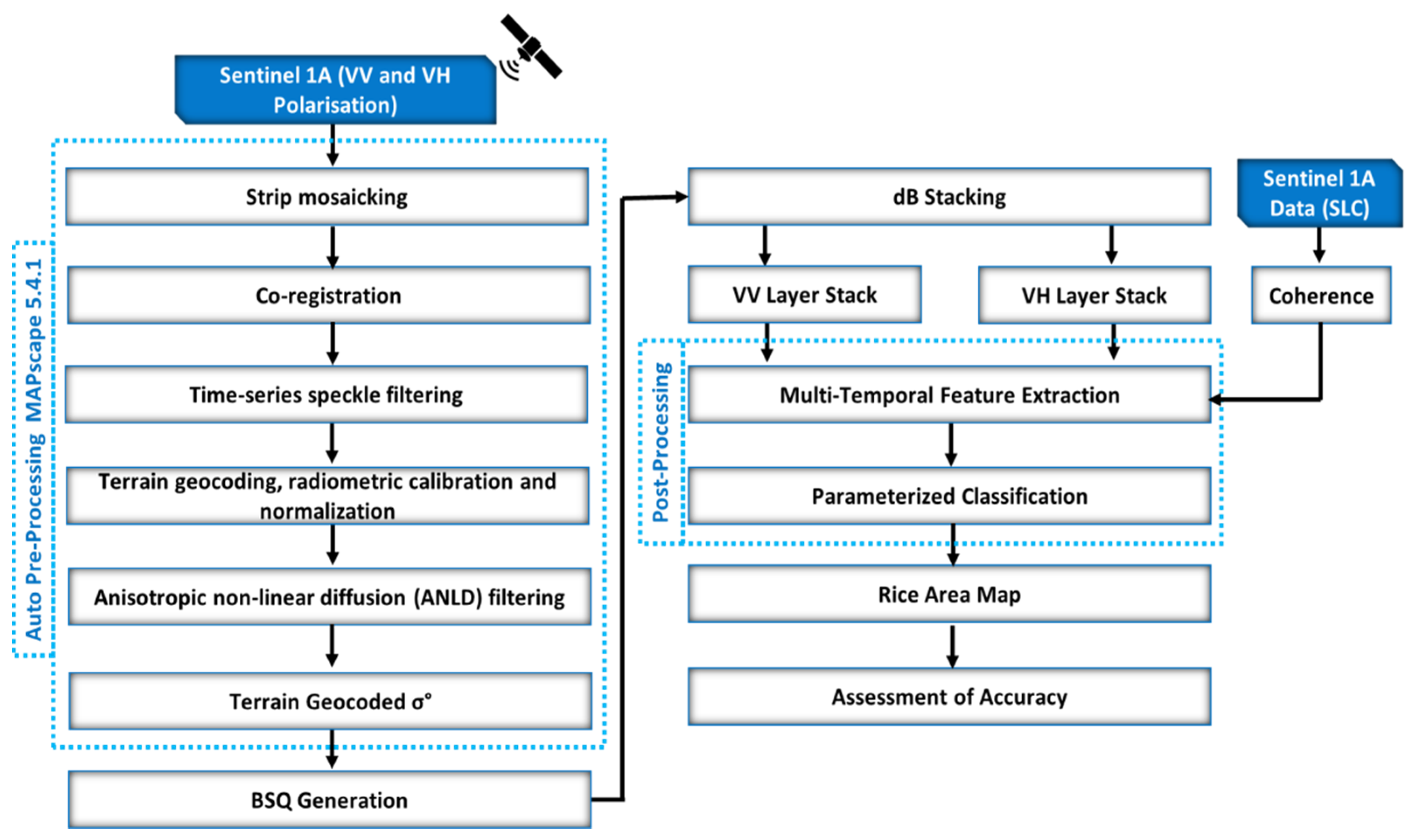
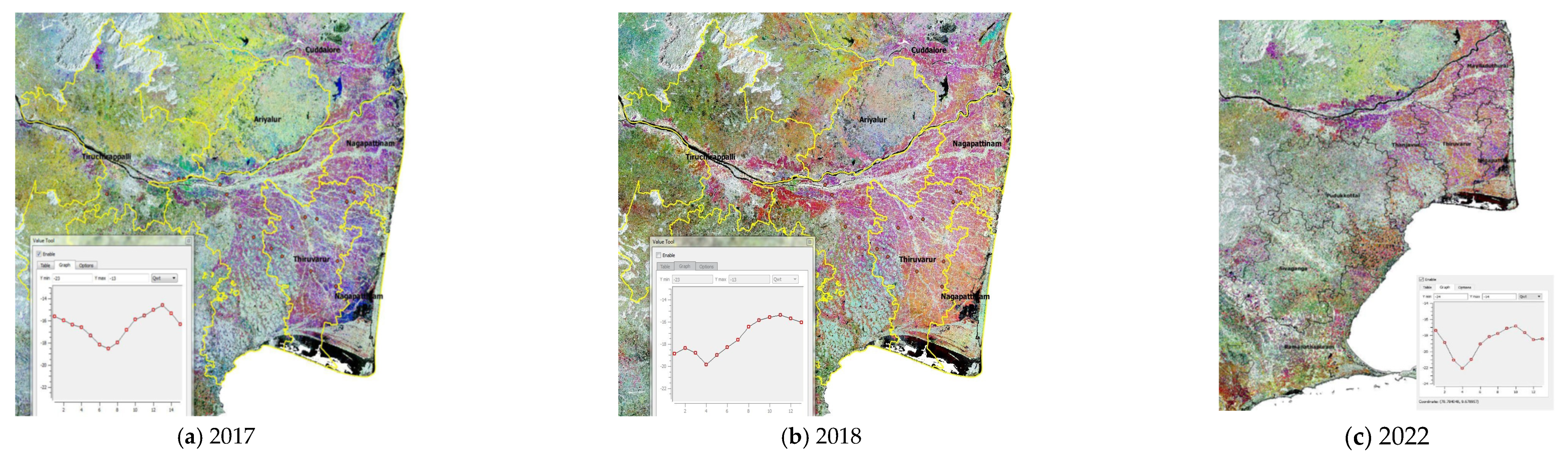
The temporal backscattering signature (σ°) for the rice crop from the study area was generated by utilizing training pixels gathered through ground truth to analyze the SAR satellite data collected during the cropping season. These signatures were converted into a dB stack created by stacking 14 and 13 acquisitions from August 2017 to January 2018 during rabi, 2017 and 16 August 2018 to 19 January 2019 during rabi, 2018. A dB stack of 13 satellite acquisitions between August 2022 and January 2023 during the samba, 2022 was generated, and the band sequential data (BSQ) are presented in Figure 6 with the temporal signature of rice crop. The backscattering curves of rice showed a minimum at the start of the season or crop emergence with a value of −20.17 dB, −20.63 dB and −20.20 dB during 2017, 2018 and 2022, respectively (Figure 7). Then, the curve showed a marginal increase in backscattering during the seedling stage and a steep increase and a peak at the flowering stage. The mean maximum values were −15.10 dB, −15.13 dB and −15.14 dB during 2017, 2018 and 2022 and are given in Table 2. Detailed analysis of backscattering signatures in the 30 test sites showed that the minimum values at the start of the season of rice ranged from −22.03 to −17.69 dB during 2017, −23.40 to −18.51 dB during 2018 and −22.24 to −20.68 during 2022. The maximum values corresponding to the flowering stage ranged from −16.10 to −14.20 dB in 2017, −17.52 to −13.62 dB in 2018 and −16.11 to −12.09 in 2022. From the seedling to the blooming stage, the rise in dB related to crop growth varied from −2.69 to −6.74 dB, with a mean value of −5.07 dB in 2017. The difference between the maximum and minimum backscattering, or the increased dB from seedling to flowering, varied from −3.61 to −7.87 dB in 2018, with a mean value of −5.50 dB. In 2022, from seedling to the flowering stage, dB values varied from −5.68 to −10.15 dB, with a mean value of −7.23 dB.

Rice Area Map

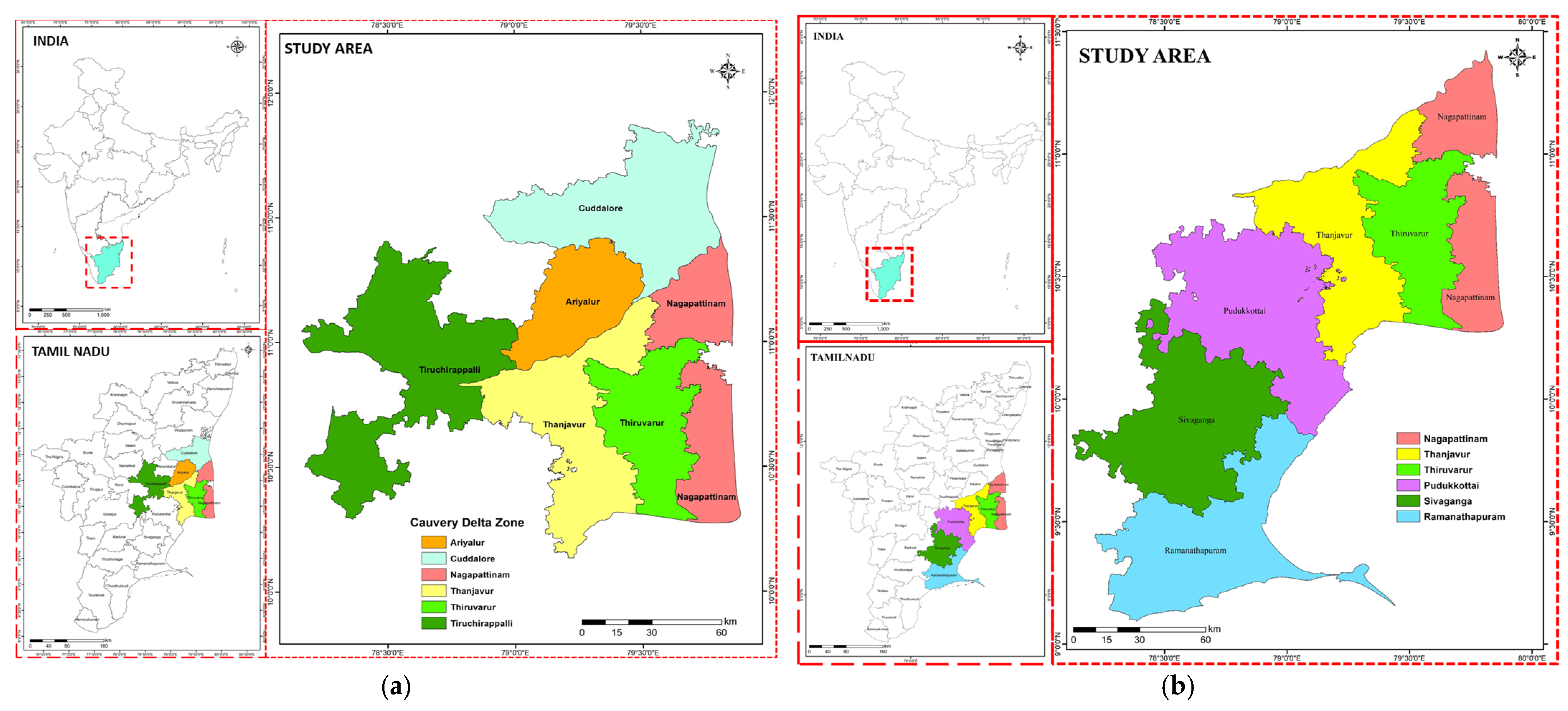
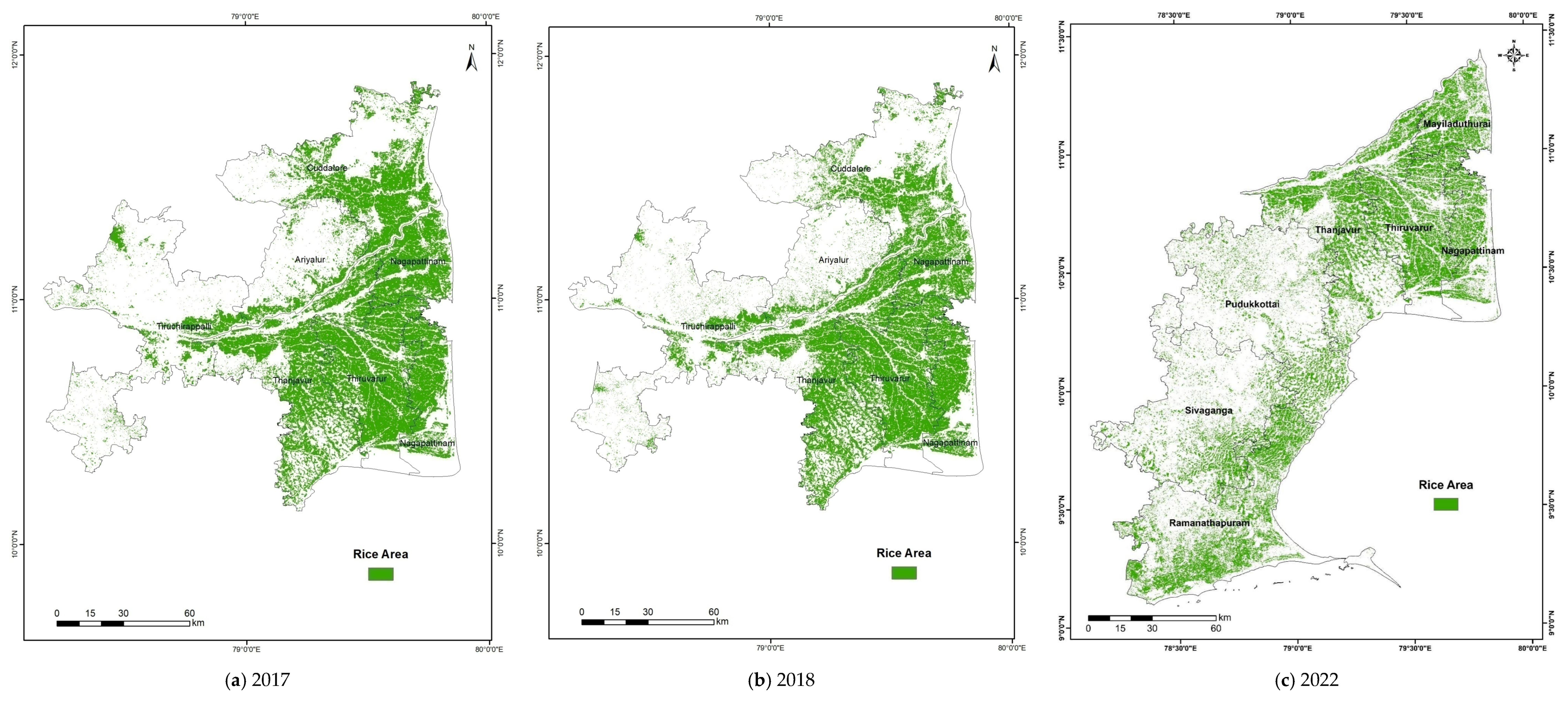
Rice area maps and statistics were derived for the study area covering six districts viz., Ariyalur, Cuddalore, Nagapattinam, Thanjavur, Thiruvarur and Tiruchirappalli in Cauvery Delta Zone during 2017–2018 and seven districts of Tamil Nadu viz., Mayiladuthurai, Nagapattinam, Thanjavur, Thiruvarur, Sivagangai, Ramanathapuram and Pudukkottai districts during 2022 using multi-temporal SAR imagery from Sentinel 1A (
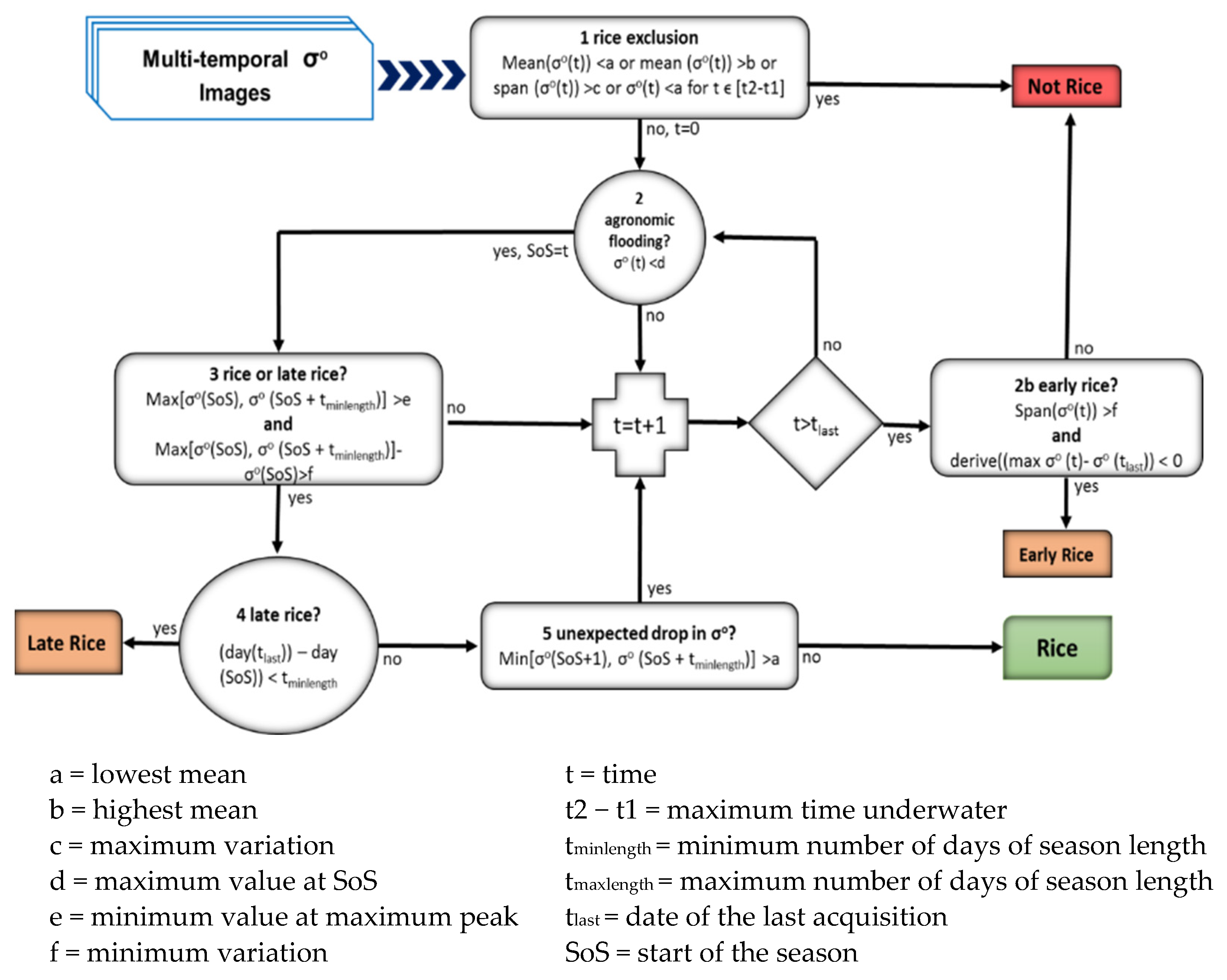
Figure 8). Late rice and early rice were combined into one class. In the study area, a total of 530,366 ha of rice area were delineated during 2017 from the multitemporal Sentinel 1A SAR data using a parameterized classification integrating multi-temporal features. The contiguous nature of the rice area facilitated an accurate estimation of the rice area in these districts, with Thiruvarur recorded as the highest area of 132,258 ha, followed by Thanjavur and Nagapattinam with an area of 126,226 and 119,411 ha, respectively. Cuddalore accounted for 99,170 ha. Tiruchirappalli and Ariyalur districts had less area under irrigation through the Cauvery River and registered an area of 31,516 and 21,785 ha, respectively.
During 2018, a total rice area of 467,134 ha across the six districts was delineated for the Cauvery delta zone. Among the districts, Thiruvarur recorded the highest area of 126,019 ha, followed by Thanjavur and Nagapattinam, with 124,618 and 105,107 ha, respectively. Cuddalore accounted for 77,312 ha. Tiruchirappalli and Ariyalur districts had less area under irrigation through the Cauvery River and registered an area of 23,545 and 10,532 ha, respectively. For the year 2022, a total rice area of 599,183 ha across the seven districts was delineated. Among the districts, Ramanathapuram recorded the highest area of 136,125 ha, followed by Thanjavur and Thiruvarur, with 117,907 and 110,512 ha, respectively. Sivagangai and Pudukkottai accounted for 66,314 ha and 65,533 ha. Mayiladuthurai and Nagapattinam districts had less area, of 54,125 ha and 48,667 ha, respectively.
A confusion matrix was formed to assess the accuracy of rice area maps by conducting ground truth collection on a rice/non-rice basis, where all land types other than rice classes were classified as non-rice classes. In total, 200 validation points covering 125 rice and 75 non-rice points were collected during 2017–2018 and used for validation of the rice area map of the Cauvery Delta Zone. In 2022, 400 validation points covering 367 rice and 33 non-rice points were used for the validation of the rice map of the study area. Rice points were classified with an accuracy of 89.6, 88.8 and 87.2 percent while non-rice points were classified with an accuracy of 98.7, 96.0 and 88.0 percent in 2017, 2018 and 2022, respectively. Considering the efficiency of the methodology utilizing SAR data, the overall accuracy was 88.5, 91.5 and 87.5 percent, with an average reliability of 88.1, 90.5 and 86.0 percent during 2017, 2018 and 2022, respectively. The kappa coefficient was 0.86, 0.83 and 0.75, indicating good accuracy levels of the products (Table 3).

3.2. Estimation of Methane Emission from Sampling Sites at Field Scale

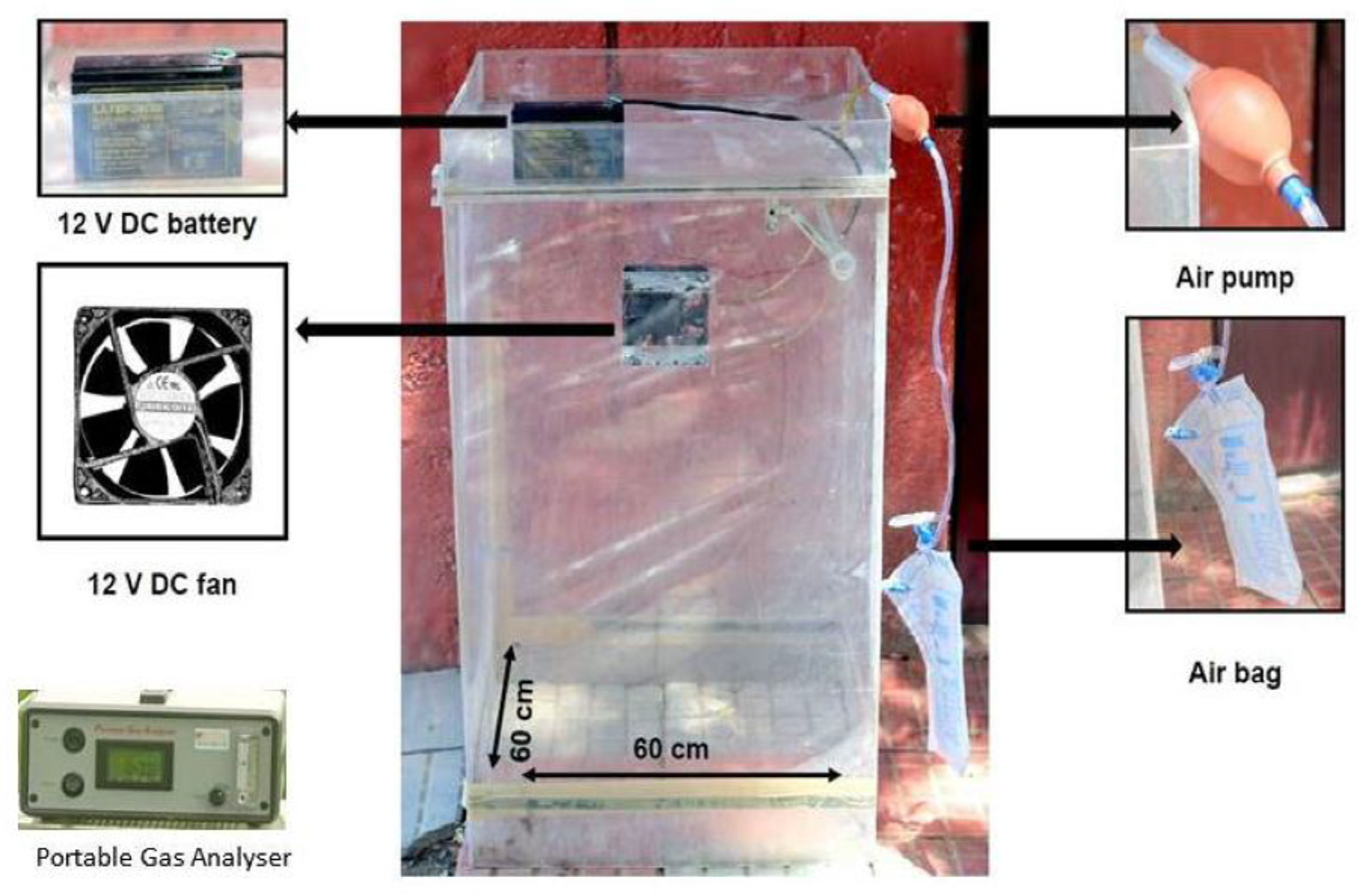
During 2017–2018 and 2022, 30 and 40 fields were continuously monitored for rice growth observations, backscattering signatures, SoS, days of flooding and estimation of methane emission spreading across the study area. Gas samples were collected at the flowering stage and analyzed for methane emission using a portable gas analyzer (Figure 9) in three locations of the sampling sites. The mean daily methane emission rates (kg/ha) for the corresponding fields are given in Table 4, Table 5 and Table 6.
The measured methane ranged from 1.68 to 3.02 ppm and 1.65 to 2.85 ppm among the 30 observed fields, with a mean of 2.20 and 2.07 ppm during 2017 and 2018, respectively. During 2022, the measured methane across 40 observed fields ranged from 3 to 12.83 ppm, with a mean of 7.04 ppm. The methane emission per day was found to be in the range of 0.37 to 0.67 kg/ha/day, 0.40 to 0.69 kg/ha/day and 0.28 to 0.46 kg/ha/day in the observation sites, with a mean of 0.50 kg/ha/day, 0.50 kg/ha/day and 0.32 kg/ha/day during 2017, 2018 and 2022. Total methane emission, which was the major contributing factor for methane flux in the atmosphere, was found to be in the range of 32.58 to 58.55 kg/ha/season, 31.94 to 55.3 kg/ha/season and 30.25 to 58.44 kg/ha/season, with a mean value of 41.7 kg/ha/season, 40.1 kg/ha/season and 42.23 kg/ha/season across the study sites during 2017, 2018 and 2022, respectively.

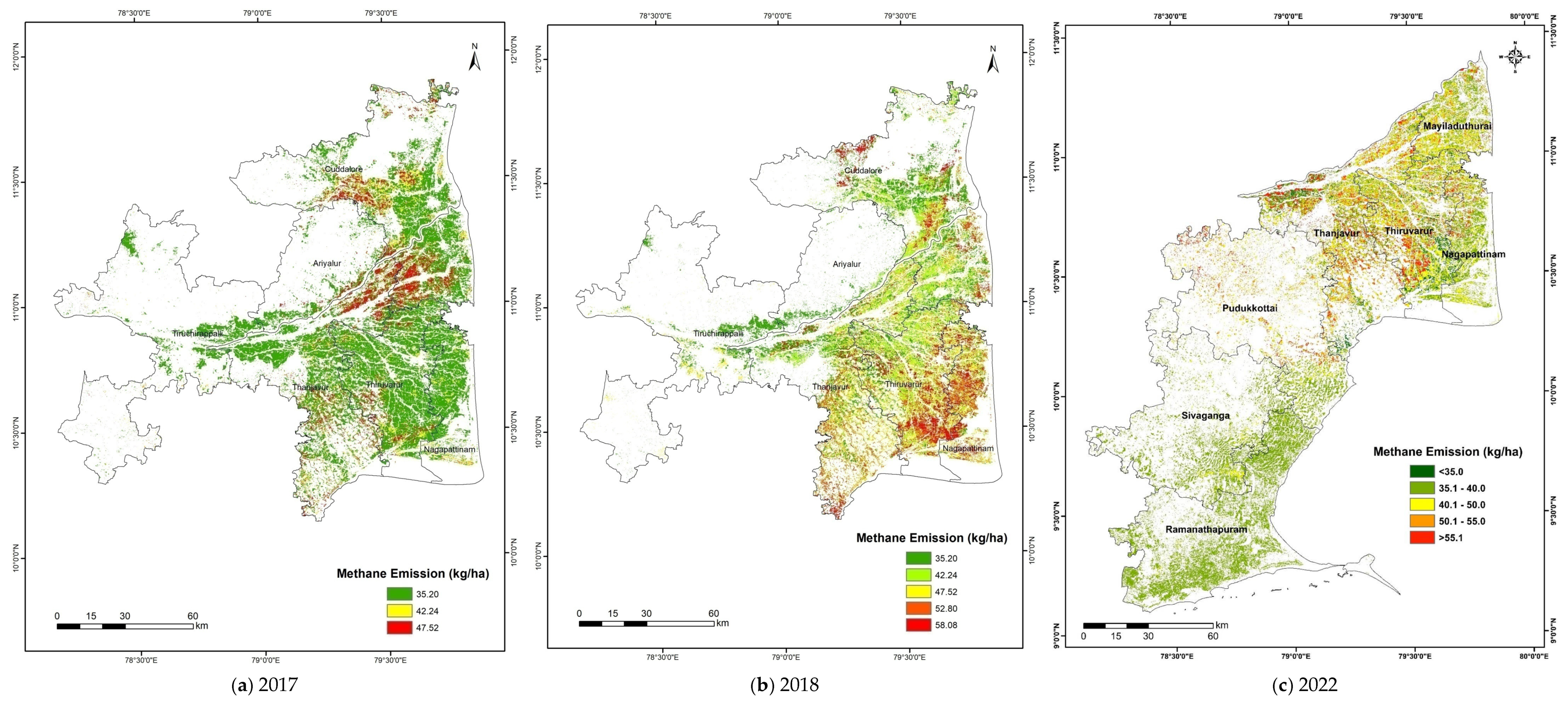
3.3. Spatial Estimation of Methane Emission Using IPCC Factor

The spatial variation in methane emission from rice fields is influenced by various agronomic and environmental factors and their interaction with the whole system involving crop, soil and atmosphere [27]. Spatial overlap of land types or crop cover types can be minimized by high-resolution satellite products. Efforts were made to integrate high-resolution Sentinel 1A data (5–20 m) and spatially estimate rice area and days of flooding to generate a regional methane emission inventory through this study (Figure 10). Further precise estimation of rice area and days after flooding could be achieved since SAR data can overcome the issue of cloud cover during the cropping season [28,
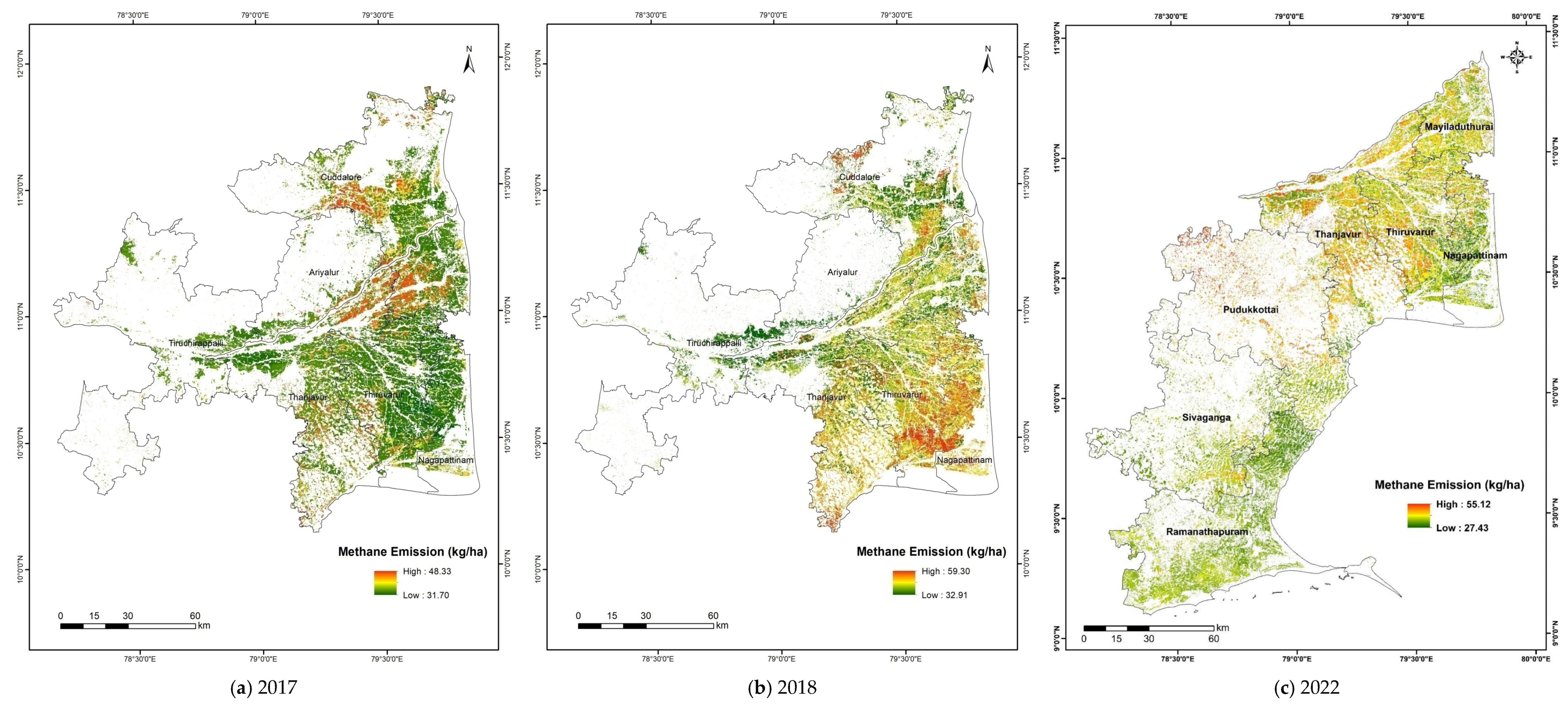
29]. Methane emission from paddy fields was estimated using the IPCC method at the district level during 2017, 2018 and 2022, and the statistics are presented in Table 7 and Table 8. The rate of methane emission was found to be in the range of 35.69 to 38.29 kg/ha, 36.23 to 45.62 kg/ha and 36.56 to 47.22 kg/ha across the districts, with a mean of 37.13 kg/ha, 42.10 kg/ha and 43.19 kg/ha during 2017, 2018 and 2022. The maximum rate of methane emission was observed in Cuddalore (38.29 kg/ha), Thiruvarur (45.62 kg/ha) and Thanjavur (47.22 kg/ha) districts during 2017, 2018 and 2022. Considering both the area and rate of methane emission, Thiruvarur district recorded the largest quantities of methane emission of 4.822 Gg from 132,258 ha of rice area at the rate of 36.46 kg/ha during 2017 and 5.749 Gg from 126,019 ha of rice area at the rate of 45.62 kg/ha during 2018. In terms of both the area and rate of methane release, the district of Thanjavur had the highest amount of methane emissions, with 5.57 Gg emitted from 117,907 ha of rice fields at a rate of 47.22 kg/ha. The cumulative methane emission assessed through the IPCC method was 19.813 Gg, 20.661 Gg and 25.72 Gg in 2017, 2018 and 2022, respectively.

3.4. Spatial Estimation of Methane Emission Using LST T-Factor

Research studies on spatial estimation of methane through satellite data mainly focus on a global scale, with coarse resolution imageries from MODIS, GOSAT, and SCIAMACHY [30,31,32]. This factor limits the utilization and inferences on emissions from different land cover types having large spatial overlaps [33]. The rate of methane emission was based on the LST T-factor method across different districts of the study area during 2017, 2018 and 2022, and is given in Table 7 and Table 8 and depicted in Figure 11. The mean values for the methane emission rate during 2017 for the study districts ranged from 34.80 to 37.50 kg/ha across the Cauvery Delta, with a mean of 36.05 kg/ha. Among the districts, Cuddalore district recorded the highest mean methane emission rate of 37.50 kg/ha, followed by Thanjavur and Ariyalur districts with the values of 36.97 and 36.08 kg/ha, respectively. Nagapattinam and Tiruchirappalli registered a mean methane emission rate of 35.80 and 35.14 kg/ha, respectively. The lowest mean rate was observed in Thiruvarur district, with a value of 34.80 kg/ha.
During the year 2018, the mean values for the rate of methane emission for the study districts ranged from 35.52 to 45.15 kg/ha across the Cauvery Delta, with a mean of 41.44 kg/ha. Among the districts, Thiruvarur district recorded the highest mean methane emission rate of 45.15 kg/ha, followed by Nagapattinam and Cuddalore districts with the values of 44.44 and 43.82 kg/ha, respectively. Thanjavur and Ariyalur districts registered a mean methane emission rate of 43.42 and 36.28 kg/ha, respectively. The lowest mean rate was observed in Tiruchirappalli district with a value of 35.52 kg/ha.
During the year 2022, the mean values for the rate of methane emission for the study districts ranged from 34.25 to 42.23 kg/ha, with a mean of 38.07 kg/ha. Among the districts, Pudukkottai district recorded the highest mean methane emission rate of 42.33 kg/ha, followed by Thanjavur and Thiruvarur districts with values of 40.98 and 38.83 kg/ha, respectively. The lowest mean rate was observed in Ramanathapuram district with a value of 34.25 kg/ha. Considering both area and rate of methane emission, Thanjavur district recorded the largest quantities of methane emission, of 4.666 Gg from 126,226 ha of rice area during 2017, and Thiruvarur district recorded 5.688 Gg from 126,019 ha of rice area during 2018. During 2022, Thanjavur district recorded the largest quantities of methane emission, of 4.83 Gg from 117,907 ha of rice area.

3.5. Validation of Methods of Methane Emission Estimation

Different methods (IPCC and LST) of estimation of methane emission from paddy fields tested during 2017, 2018 and 2022 were validated against the observed values from the sampling sites, and the statistical parameters RMSE, NRMSE and percent agreement were worked out and given in Table 9. The comparison of values for methane emission using IPCC and observed values resulted in a mean RMSE of 6.80, 3.38 and 8.04 kg/ha and NRMSE of 14.29, 8.68 and 19.75 percent, respectively. The percent agreement mean was 85.7, 91.32 and 80.25 percent during 2017, 2018 and 2022, respectively. Using the LST factor, the mean RMSE values recorded were 7.71, 3.31 and 6.70 kg/ha, and those of NRMSE were 16.31, 8.57 and 15.31 percent, with the agreement of 83.69, 91.43 and 84.69 percent during 2017, 2018 and 2022, respectively.

4. Discussion

4.1. Radar Backscattering Signature

The primary variation corresponds to the growth from seedling to the maximum tillering stage; as the growth advanced, the backscatter from the rice crop increased till the flowering stage. In all of the fields, the values tended to drop farther from flowering to maturity. Significant temporal behavior and a large dynamic range (−20.63 to −15.10 dB) during the growth period were observed by many researchers [34,35,36]. Moreover, short wavelengths, especially at a larger incident angle, were sensitive enough to detect even very small rice seedlings just after transplanting. The correlation between σo and rice biophysical parameters showed that lower frequencies (X-band) were more closely related to fresh weight, LAI and plant weight than other parameters. On the other hand, σo derived from the C band can provide information on par with NDVI [37].

Rice Area Estimation

SAR sensors have great potential in precisely detecting rice fields due to specular features exhibited under flooded surface conditions [38]. Many researchers have shown interest in better understanding the relationships between backscatter and crop growth and applying them to detect rice and monitor crop growth [39,40]. The rice area was estimated [41] using the land surface water index (LSWI) and enhanced vegetation index (EVI), and the high-temperature damaged rice area was mapped by integrating the rice map with MODIS LST, vegetation indices, DEM data and daily maximum–minimum air temperature. It was validated using certified agriculture statistics with an error rate under 8 percent. Landsat is primarily used in many remote sensing data observations but lacks quality parameters due to cloud cover and other factors. A phenology-based algorithm combining Landsat and MODIS data was used [42] in southern China to map paddy and multi-cropping patterns. In Poyang Lake Plain, the algorithm produced 93.66 percent overall accuracy and a kappa coefficient of 0.85 compared to ground truth data.
AL-Zubaidi [43] analyzed nine vegetation indices to identify excellent vegetation spectral indices for rice area estimation. The result showed that the rice growth vegetation index (RGVI) had the lowest error rate predicted (4.3 percent) against reference data, while the infrared percentage vegetation index (IPVI) predicted the highest error rate of 30.3 percent for rice area mapping. The rice area was estimated [44] using Sentinel 2 satellite data and the supervised closest neighborhood object-based classification approach. The overall accuracy of 95 percent and the kappa coefficient of 0.93 were achieved through this method. All of the preceding research was carried out utilizing optical data, which was unsuitable during the monsoon seasons due to approximately 90 percent of the data being obscured by clouds. Consequently, we turned to Sentinel 1A SAR microwave data, capable of penetrating clouds, enabling us to delineate the rice area with greater precision.

4.2. Estimation of Methane Emission

Methane emission from rice fields was directly proportional to the area under the rice culture type and total crop duration. Earlier allocations of areas to rice cultural types were based on statistical data for harvested rice areas or country-specific reports to calculate the methane emission values [10,12,45]. Changes in agronomic and environmental factors and their interaction with the system determined the methane emission [46]. Chhabra et al. [47,48] generated the spatial and temporal pattern of methane emission from the rice fields of India using satellite remote sensing and Geographic Information System (GIS) techniques. Multidate SPOT VGT 10-day NDVI composite data for a whole year were used to map the rice area and delineate single- and double-cropped rice areas, crop calendar and growth stages.

5. Conclusions

This study introduced a state-of-the-art methodology for methane emission estimation in rice cultivation, leveraging multi-temporal C-band synthetic aperture radar (SAR) data from Sentinel-1A along with advanced processing techniques, employed to estimate methane emissions over major rice growing areas in Tamil Nadu. The proposed methodology excels in its precision and adaptability, utilizing advanced processing techniques and innovative approaches. This research delved into the backscattering signature (σ°) of rice crops, using ground truth data and SAR satellite information from cropping seasons. The temporal backscattering curves revealed distinctive patterns, with minimum values at crop emergence at the start of the season or crop emergence with a value of −20.17 dB, −20.63 dB and −20.20 dB during 2017, 2018 and 2022, respectively, and peak values during flowering. Then, the curve showed a marginal increase in backscattering during the seedling stage and a steep increase and a peak at the flowering stage. Rice area maps and statistics were generated for the Cauvery Delta Zone (2017–2018) and Tamil Nadu (2022). In 2017, the study identified 530,366 hectares of rice area, with Thiruvarur having the largest at 132,258 hectares. By 2018, the total area was 467,134 hectares, and Thiruvarur led again with 126,019 hectares. In 2022, across seven districts, Ramanathapuram recorded the largest rice area at 136,125 hectares. Thanjavur and Thiruvarur followed with 117,907 and 110,512 ha. Validation points and a confusion matrix demonstrated the accuracy of rice area maps, with an overall accuracy ranging from 88.5% to 91.5% during different years. The kappa coefficient affirmed the reliability of the methodology. This comprehensive approach utilizing SAR data provides valuable insights into monitoring and managing rice cultivation in the region. Beyond rice area mapping, the methodology extended to estimating methane emissions by using the IPCC factor and land surface temperature (LST) T-factor methods, providing valuable insights into the spatial and temporal patterns of greenhouse gas emissions from rice fields.
Methane emissions were spatially estimated at the district level, indicating variations across districts and years. In 2017, the emissions ranged from 35.69 to 38.29 kg/ha, totaling 19.813 Gg. In 2018, the range was 36.23 to 45.62 kg/ha, totaling 20.661 Gg. In 2022, emissions varied from 36.56 to 47.22 kg/ha, totaling 25.72 Gg. The LST method showed rates ranging from 34.80 to 37.50 kg/ha in 2017, 35.52 to 45.15 kg/ha in 2018, and 28.8 to 51.4 kg/ha in 2022. Validation against observed values indicated the reliability of both methods, with the IPCC method showing mean RMSE of 6.80, 3.38, and 8.04 kg/ha in 2017, 2018, and 2022, respectively. The LST method had mean RMSE of 7.71, 3.31, and 6.70 kg/ha for the same years. Overall, this study contributes valuable insights into the spatial and temporal dynamics of methane emissions from rice cultivation, offering a scientific basis for informed decision-making, policy-making and the development of effective mitigation strategies in the context of global climate change.

Author Contributions

Conceptualization, N.S.S.; Data curation, N.S.S.; Formal analysis, N.S.S., M.D., K.R., A.P.S. and P.S.; Funding acquisition, S.P. and V.G.; Investigation, S.P., K.R. and A.P.S.; Methodology, N.S.S.; Project administration, S.P. and V.G.; Resources, S.P.; Software, N.S.S.; Supervision, S.P., V.G., K.R. and A.P.S.; Validation, N.S.S.; Visualization, K.R.; Writing—original draft, N.S.S.; Writing—review and editing, N.S.S., M.D. and P.S. All authors have read and agreed to the published version of the manuscript.

Funding

This research received external funding from the World Bank, Tamil Nadu Irrigated Agriculture Modernization Project (Grant number IFHRMS DPC No. 2415-01-120-PF30903).

Institutional Review Board Statement

Not applicable.

Data Availability Statement

All relevant data are included in the manuscript.

Acknowledgments

The authors thank the Department of Remote Sensing & GIS, Tamil Nadu Agricultural University, Coimbatore, for extending their guidance and technical assistance in conducting this research work.

Conflicts of Interest

The authors declare no conflicts of interest related to this article.

References

  1. Zhang, B.; Tian, H.; Ren, W.; Tao, B.; Lu, C.; Yang, J.; Banger, K.; Pan, S. Methane emissions from global rice fields: Magnitude, spatiotemporal patterns, and environmental controls. Glob. Biogeochem. Cycles 2016, 30, 1246–1263. [Google Scholar] [CrossRef]
  2. Chen, H.; Yu, C.; Li, C.; Xin, Q.; Huang, X.; Zhang, J.; Yue, Y.; Huang, G.; Li, X.; Wang, W. Modeling the impacts of water and fertilizer management on the ecosystem service of rice rotated cropping systems in China. Agric. Ecosyst. Environ. 2016, 219, 49–57. [Google Scholar] [CrossRef]
  3. FAO. Socio-Economic Analysis and Policy Implications of the Roles of Agriculture in Developing Countries; Original edition, Summary report, roles of agriculture project; FAO: Rome, Italy, 2014. [Google Scholar]
  4. Maclean, J.; Hardy, B.; Hettel, G. Rice Almanac; Source Book for One of the Most Important Economic Activities on Earth; IRRI: Los Baños, Philippines, 2013. [Google Scholar]
  5. US Environmental Protection Agency. Global Mitigation of Non-CO2 Greenhouse Gases. EPA 430-R-06-005; US Environmental Protection Agency: Washington, DC, USA, 2006.
  6. Houghton, J.E.T.; Ding, Y.; Griggs, D.; Noguer, M.; van der Linden, P.; Dai, X.; Maskell, M.; Johnson, C. Climate Change 2001: The Scientific Basis; Cambridge University Press: Cambridge, UK, 2001; p. 881. [Google Scholar]
  7. Wassmann, R.; Aulakh, M.S. The role of rice plants in regulating mechanisms of methane emissions. Biol. Fertil. Soils 2000, 31, 20–29. [Google Scholar] [CrossRef]
  8. Wahlen, M.; Tanaka, N.; Henry, R.; Deck, B.; Zeglen, J.; Vogel, J.S.; Southon, J.; Shemesh, A.; Fairbanks, R.; Broecker, W. Carbon-14 in methane sources and in atmospheric methane: The contribution from fossil carbon. Science 1989, 245, 286–290. [Google Scholar] [CrossRef] [PubMed]
  9. Huke, R.E. Rice Area by Type of Culture: South, Southeast, and East Asia; International Rice Research Institute: Los Baños, Philippines, 1982. [Google Scholar]
  10. Gupta, P.K.; Sharma, C.; Bhattacharya, S.; Mitra, A.P. Scientific basis for establishing country greenhouse gas estimates for rice-based agriculture: An Indian case study. Nutr. Cycl. Agroecosyst. 2002, 64, 19–31. [Google Scholar] [CrossRef]
  11. Solomon, S.; Qin, D.; Manning, M.; Averyt, K.; Marquis, M. Climate Change 2007-the Physical Science Basis: Working Group I Contribution to the Fourth Assessment Report of the IPCC; Cambridge University Press: Cambridge, UK, 2007; Volume 4. [Google Scholar]
  12. Yan, X.; Akiyama, H.; Yagi, K.; Akimoto, H. Global estimations of the inventory and mitigation potential of methane emissions from rice cultivation conducted using the 2006 Intergovernmental Panel on Climate Change Guidelines. Glob. Biogeochem. Cycles 2009, 23. [Google Scholar] [CrossRef]
  13. Kahle, A.B. Surface emittance, temperature, and thermal inertia derived from Thermal Infrared Multispectral Scanner (TIMS) data for Death Valley, California. Geophysics 1987, 52, 858–874. [Google Scholar] [CrossRef]
  14. Holecz, F.; Barbieri, M.; Collivignarelli, F.; Gatti, L.; Nelson, A.; Setiyono, T.D.; Boschetti, M.; Manfron, G.; Brivio, P.A.; Quilang, J. An operational remote sensing based service for rice production estimation at national scale. In Proceedings of the Living Planet Symposium, Edinburgh, UK, 9–13 September 2013. [Google Scholar]
  15. Confalonieri, R.; Francone, C.; Foi, M. The PocketLAI smartphone app: An alternative method for leaf area index estimation. Agric. For. Meteorol. 2014. Available online: https://scholarsarchive.byu.edu/iemssconference/2014/Stream-A/41/ (accessed on 15 April 2023).
  16. Lantin, R.S.; Aduna, J.B.; Javellana, A.M. Methane Measurements in Rice Fields; International Rice Research Institute: Los Baños, Philippines, 1995. [Google Scholar]
  17. Rolston, D. Gas flux. In Methods of Soil Analysis, 2nd ed.; Klute, A., Ed.; American Society of Agronomy-Soil Science Society of America: Madison, WI, USA, 1986. [Google Scholar]
  18. Richards, J.A.; Richards, J. Remote Sensing Digital Image Analysis; Springer: Berlin/Heidelberg, Germany, 1999; Volume 3. [Google Scholar]
  19. Liu, J. Macro-Scale Survey and Dynamic Study of Natural Resources and Environment of China by Remote Sensing; China Science and Technology Press: Beijing, China, 1996; pp. 113–124. [Google Scholar]
  20. Li, C. Modeling trace gas emissions from agricultural ecosystems. In Methane Emissions from Major Rice Ecosystems in Asia; Springer: Berlin/Heidelberg, Germany, 2000; pp. 259–276. [Google Scholar]
  21. Li, C.; Frolking, S.; Crocker, G.J.; Grace, P.R.; Klír, J.; Körchens, M.; Poulton, P.R. Simulating trends in soil organic carbon in long-term experiments using the DNDC model. Geoderma 1997, 81, 45–60. [Google Scholar] [CrossRef]
  22. Li, C.; Frolking, S.; Harriss, R. Modeling carbon biogeochemistry in agricultural soils. Glob. Biogeochem. Cycles 1994, 8, 237–254. [Google Scholar] [CrossRef]
  23. Le Toan, T.; Ribbes, F.; Wang, L.-F.; Floury, N.; Ding, K.-H.; Kong, J.A.; Fujita, M.; Kurosu, T. Rice crop mapping and monitoring using ERS-1 data based on experiment and modeling results. IEEE Trans. Geosci. Remote Sens. 1997, 35, 41–56. [Google Scholar] [CrossRef]
  24. Suga, Y.; Konishi, T. Rice crop monitoring using X, C and L band SAR data. In Remote Sensing for Agriculture, Ecosystems, and Hydrology X; SPIE: Bellingham, WA, USA, 2008; pp. 305–314. [Google Scholar]
  25. Nelson, A.; Setiyono, T.; Rala, A.; Quicho, E.; Raviz, J.; Abonete, P.; Maunahan, A.; Garcia, C.; Bhatti, H.; Villano, L.S. Towards an operational SAR-based rice monitoring system in Asia: Examples from 13 demonstration sites across Asia in the RIICE project. Remote Sens. 2014, 6, 10773–10812. [Google Scholar] [CrossRef]
  26. Setiyono, T.D.; Quicho, E.D.; Gatti, L.; Campos-Taberner, M.; Busetto, L.; Collivignarelli, F.; García-Haro, F.; Boschetti, M.; Khan, N.; Holecz, F. Spatial rice yield estimation based on MODIS and Sentinel-1 SAR data and ORYZA crop growth model. Remote Sens. 2018, 10, 293. [Google Scholar] [CrossRef]
  27. Wang, M.; Li, J. CH4 emission and oxidation in Chinese rice paddies. Nutr. Cycl. Agroecosyst. 2002, 64, 43–55. [Google Scholar]
  28. Setiyono, T.D.; Holecz, F.; Khan, N.I.; Barbieri, M.; Quicho, E.; Collivignarelli, F.; Maunahan, A.; Gatti, L.; Romuga, G.C. Synthetic Aperture Radar (SAR)-based paddy rice monitoring system: Development and application in key rice producing areas in Tropical Asia. In IOP Conference Series: Earth and Environmental Science; IOP Publishing: Bristol, UK, 2017; p. 012015. [Google Scholar]
  29. Sudarmanian, N.S.; Pazhanivelan, S.; Ragunath, K.P. Remote Sensing based Methane Emission from Rice Fields in Tiruchirapalli District. Madras Agric. J. 2017, 104, 1–3. [Google Scholar]
  30. Bergamaschi, P.; Houweling, S.; Segers, A.; Krol, M.; Frankenberg, C.; Scheepmaker, R.A.; Dlugokencky, E.; Wofsy, S.C.; Kort, E.A.; Sweeney, C. Atmospheric CH4 in the first decade of the 21st century: Inverse modeling analysis using SCIAMACHY satellite retrievals and NOAA surface measurements. J. Geophys. Res. Atmos. 2013, 118, 7350–7369. [Google Scholar] [CrossRef]
  31. Alexe, M.; Bergamaschi, P.; Segers, A.; Detmers, R.; Butz, A.; Hasekamp, O.; Guerlet, S.; Parker, R.; Boesch, H.; Frankenberg, C. Inverse modelling of CH4 emissions for 2010–2011 using different satellite retrieval products from GOSAT and SCIAMACHY. Atmos. Chem. Phys. 2014, 14, 11493–11539. [Google Scholar]
  32. Wecht, K.J.; Jacob, D.J.; Sulprizio, M.P.; Santoni, G.W.; Wofsy, S.C.; Parker, R.; Bösch, H.; Worden, J. Spatially Resolving Methane Emissions in California: Constraints from the CalNex Aircraft Campaign and from Present (GOSAT, TES) and Future (TROPOMI, Geostationary) Satellite Observations. Atmos. Chem. Phys. 2014, 14, 8173–8184. [Google Scholar] [CrossRef]
  33. Fung, I.; John, J.; Lerner, J.; Matthews, E.; Prather, M.; Steele, L.; Fraser, P. Three-dimensional model synthesis of the global methane cycle. J. Geophys. Res. Atmos. 1991, 96, 13033–13065. [Google Scholar] [CrossRef]
  34. Inoue, Y.; Kurosu, T.; Maeno, H.; Uratsuka, S.; Kozu, T.; Dabrowska-Zielinska, K.; Qi, J. Season-long daily measurements of multifrequency (Ka, Ku, X, C, and L) and full-polarization backscatter signatures over paddy rice field and their relationship with biological variables. Remote Sens. Environ. 2002, 81, 194–204. [Google Scholar] [CrossRef]
  35. Oh, Y.; Hong, S.-Y.; Kim, Y.; Hong, J.-Y.; Kim, Y.-H. Polarimetric backscattering coefficients of flooded rice fields at L- and C-bands: Measurements, modeling, and data analysis. IEEE Trans. Geosci. Remote Sens. 2009, 47, 2714–2721. [Google Scholar]
  36. Kim, Y.-H.; Hong, S.-Y.; Lee, H.-Y. Estimation of Paddy Rice Growth Parameters Using L, C, X-Bands Polarimetric Scatterometer. Korean J. Remote Sens. 2009, 25, 31–44. [Google Scholar]
  37. Inoue, Y.; Sakaiya, E.; Wang, C. Capability of C-Band Backscattering Coefficients from High-Resolution Satellite SAR Sensors to Assess Biophysical Variables in Paddy Rice. Remote Sens. Environ. 2014, 140, 257–266. [Google Scholar] [CrossRef]
  38. Choudhury, I.; Chakraborty, M.; Santra, S.C.; Parihar, J.S. Methodology to classify rice cultural types based on water regimes using multi-temporal RADARSAT-1 data. Int. J. Remote Sens. 2012, 33, 4135–4160. [Google Scholar] [CrossRef]
  39. Sudarmanian, N.S.; Pazhanivelan, S.; Panneerselvam, S. Estimation of methane emission from paddy fields using SAR and MODIS satellite data. J. Agrometeorol. 2019, 21, 102–109. [Google Scholar]
  40. Pazhanivelan, S.; Geethalakshmi, V.; Tamilmounika, R.; Sudarmanian, N.S.; Kaliaperumal, R.; Ramalingam, K.; Sivamurugan, A.P.; Mrunalini, K.; Yadav, M.K.; Quicho, E.D. Spatial Rice Yield Estimation Using Multiple Linear Regression Analysis, Semi-Physical Approach and Assimilating SAR Satellite Derived Products with DSSAT Crop Simulation Model. Agronomy 2022, 12, 2008. [Google Scholar] [CrossRef]
  41. Dou, Y.; Huang, R.; Mansaray, L.R.; Huang, J. Mapping high temperature damaged area of paddy rice along the Yangtze River using Moderate Resolution Imaging Spectroradiometer data. Int. J. Remote Sens. 2020, 41, 471–486. [Google Scholar] [CrossRef]
  42. Ding, M.; Guan, Q.; Li, L.; Zhang, H.; Liu, C.; Zhang, L. Phenology-based rice paddy mapping using multi-source satellite imagery and a fusion algorithm applied to the Poyang Lake plain, Southern China. Remote Sens. 2020, 12, 1022. [Google Scholar] [CrossRef]
  43. AL-Zubaidi, R.A.A. Determination the Best Vegetation Spectral Indices for Estimating Rice Crop Area in the Kefal Shinafiya Project in Iraq. Iraqi J. Sci. Technol. 2020, 11, 53–59. [Google Scholar]
  44. Ali, A.M.; Savin, I.; Poddubskiy, A.; Abouelghar, M.; Saleh, N.; Abutaleb, K.; El-Shirbeny, M.; Dokukin, P. Integrated method for rice cultivation monitoring using Sentinel-2 data and Leaf Area Index. Egypt. J. Remote Sens. Space Sci. 2021, 24, 431–441. [Google Scholar] [CrossRef]
  45. Griggs, D.J.; Noguer, M. Climate change 2001: The scientific basis. Contribution of Working Group I to the Third Assessment Report of the Intergovernmental Panel on Climate Change. Int. J. Epidemiol. 2003, 32, 321. [Google Scholar] [CrossRef]
  46. Le Mer, J.; Roger, P. Production, oxidation, emission and consumption of methane by soils: A review. Eur. J. Soil Biol. 2001, 37, 25–50. [Google Scholar] [CrossRef]
  47. Chhabra, A.; Manjunath, K.R.; Panigrahy, S.; Parihar, J.S. Methane Emission Inventory from Indian Livestock; Scientific Report; Space Applications Centre: Ahmedabad, India, 2008; SAC/AFEG/AMD/EIAA/SN/01/08; p. 51.
  48. Wang, L.; Qiu, J.; Tang, H.; Li, H.; Li, C.; Van Ranst, E. Modelling soil organic carbon dynamics in the major agricultural regions of China. Geoderma 2008, 147, 47–55. [Google Scholar] [CrossRef]
Figure 1. (a) Study area for the years 2017 and 2018; (b) study area for the year 2022.
Agriculture 14 00496 g001
Figure 2. Crop Calendar of rice in the study area.
Agriculture 14 00496 g002
Figure 3. Flow chart depicting the methodology of SAR processing and rice area mapping.
Agriculture 14 00496 g003
Figure 4. MAPscape-RICE: A rule-based rice detection system for multi-temporal C-band σ°.
Agriculture 14 00496 g004
Figure 5. The flow chart outlines the general approach for estimating methane emissions.
Agriculture 14 00496 g005
Figure 6. dB stack generated with Sentinel-1A data and rice temporal signature.
Agriculture 14 00496 g006
Figure 7. Temporal dB curves for rice using Sentinel 1A data.
Agriculture 14 00496 g007
Figure 8. Rice area map of Cauvery Delta Zone.
Agriculture 14 00496 g008
Figure 9. Static closed chamber for collecting methane.
Agriculture 14 00496 g009
Figure 10. IPCC factor-based methane emission (kg/ha) from rice fields in Cauvery Delta Zone.
Agriculture 14 00496 g010
Figure 11. LST T-factor based methane emission (kg/ha) from rice fields in Cauvery Delta Zone.
Agriculture 14 00496 g011
Table 1. Selection criteria are based on temporal features and site-specific parameters for the rule-based categorization.
ParameterRelationship between Parameter and Temporal Feature
a = lowest meana < (i) minimum of the mean σ° across all rice signatures
b = highest meanb > (ii) maximum of the mean σ° across all rice signatures
c = maximum variationc > (vi) maximum of the range in σ° across all rice signatures
d = max value at SoSd > (iii) highest minimum in σ° across all rice signatures
e = min value at peake < (iv) lowest maximum in σ° across all rice signatures
f = minimum variationf < (v) minimum of the range in σ° across all rice signatures
Table 2. Temporal dB value for rice crop for the years 2017, 2018 and 2022.
201720182022
S.NoDate of AcquisitiondB ValueDate of AcquisitiondB ValueDate of AcquisitiondB Value
126-Sep−18.6916-Aug−19.9019-Aug−16.90
208-Oct−20.0328-Aug−21.2731-Aug−17.98
320-Oct−21.1609-Sep−21.0012-Sep−19.01
408-Nov−20.6321-Sep−19.8124-Sep−19.67
501-Nov−20.1603-Oct−18.5606-Oct−19.50
613-Nov−19.5927-Oct−17.4730-Oct−18.17
725-Nov−18.2608-Nov−16.4211-Nov−16.96
807-Dec−17.5720-Nov−14.8123-Nov−16.10
919-Dec−16.9102-Dec−14.2205-Dec−15.55
1031-Dec−16.1814-Dec−14.5817-Dec−15.20
1112-Jan−16.1628-Dec−16.0229-Dec−14.71
12--07-Jan−18.8810-Jan−14.15
13--19-Jan−19.7322-Jan−14.88
Table 3. Confusion matrix for accuracy assessment of rice classification during 2017, 2018 and 2022.
Actual class from the surveyPredicted class from the map
201720182022
ClassRiceNon-RiceAccuracy (%)RiceNon-RiceAccuracy (%)RiceNon-RiceAccuracy (%)
Rice1121389.61111488.82253387.2
Non-rice17498.737296.01712588.0
Reliability (%)99.077.19397.483.791.593.079.187.5
Average accuracy (%)90.5 92.4 87.6
Average reliability (%)88.1 90.5 86.0
Overall accuracy (%)88.5Good Accuracy91.5Good Accuracy87.5Good Accuracy
Kappa index0.860.830.75
Table 4. Field-level estimation of methane emission during 2017.
S.No.PlaceDistrictMethane Measured (ppm)Methane Emission (kg/ha/day)Total Methane Emission (kg/ha/season)
1.PalayangudiThiruvarur2.150.4841.61
2.KeeramberNagapattinam2.070.4640.18
3.AdichapuramThiruvarur2.020.4539.23
4.KarikottaiThiruvarur2.040.4539.48
5.VaduvurAgraharamThiruvarur2.010.4538.91
6.RaghavambalpuramThanjavur1.880.4236.46
7.AnthagudiNagapattinam2.120.4741.13
8.KatturThanjavur1.940.4337.51
9.ADAC & RI Tiruchirappalli1.840.4135.70
10.NavalurkottapattuTiruchirappalli2.380.5346.18
11.Aravoor,Thiruvarur1.680.3732.58
12.PerumburThanjavur1.930.4337.40
13.KudalurThanjavur1.840.4135.70
14.SimizhiThiruvarur1.780.4034.57
15.UthirangudiThiruvarur2.530.5649.02
16.VaragurThanjavur2.460.5547.60
17.MelatturThanjavur3.000.6758.04
18.TirukkannapuramNagapattinam2.600.5850.46
19.KeelanbilTiruchirappalli1.860.4136.02
20.AriyurTiruchirappalli1.740.3933.66
21.AdikudiTiruchirappalli1.840.4135.67
22.ThiruvaiyaruThanjavur3.000.6758.14
23.AmbalNagapattinam3.020.6758.55
24.PalinganathamAriyalur2.150.4841.74
25.BapurasapuramThanjavur2.210.4942.76
26.KatchukattuThanjavur1.750.3933.86
27.EdakkudiNagapattinam2.590.5850.15
28.AnnavasalNagapattinam2.480.5548.03
29.TiruchampalliNagapattinam1.960.4437.94
30.VanadirajapuramNagapattinam1.750.3934.00
Mean2.200.541.7
Minimum1.680.3732.58
Maximum3.020.6758.55
Table 5. Field-level estimation of methane emission during 2018.
S.No.PlaceDistrictMethane Measured (ppm)Methane Emission (kg/ha/day)Total Methane Emission (kg/ha/season)
1.PalayangudiThiruvarur2.010.4938.9
2.KeeramberNagapattinam1.940.4737.6
3.AdichapuramThiruvarur1.890.4636.7
4.KarikottaiThiruvarur1.980.4838.3
5.VaduvurAgraharamThiruvarur1.950.4737.8
6.RaghavambalpuramThanjavur1.790.4334.7
7.AnthagudiNagapattinam2.020.4939.2
8.KatturThanjavur1.840.4535.7
9.ADAC & RI Tiruchirappalli1.810.4435.0
10.NavalurkottapattuTiruchirappalli2.340.5745.3
11.Aravoor,Thiruvarur1.650.4031.9
12.PerumburThanjavur1.890.4636.7
13.KudalurThanjavur1.810.4435.0
14.SimizhiThiruvarur1.750.4233.9
15.UthirangudiThiruvarur2.480.6048.1
16.VaragurThanjavur2.410.5846.7
17.MelatturThanjavur2.850.6955.3
18.TirukkannapuramNagapattinam2.480.6048.1
19.KeelanbilTiruchirappalli1.770.4334.3
20.AriyurTiruchirappalli1.650.4032.1
21.AdikudiTiruchirappalli1.720.4233.3
22.ThiruvaiyaruThanjavur2.800.6854.3
23.AmbalNagapattinam2.820.6854.7
24.PalinganathamAriyalur2.070.5040.1
25.BapurasapuramThanjavur2.120.5141.1
26.KatchukattuThanjavur1.680.4132.6
27.EdakkudiNagapattinam2.540.6149.2
28.AnnavasalNagapattinam2.430.5947.1
29.TiruchampalliNagapattinam1.920.4637.2
30.VanadirajapuramNagapattinam1.720.4233.3
Mean2.070.5040.13
Minimum1.650.4031.94
Maximum2.850.6955.28
Table 6. Field-level estimation of methane emission during 2022.
S.NoPlaceDistrictMethane Measured (ppm)Methane Emission (kg/ha/day)Total Methane Emission (kg/ha/season)
1.Visavanoor Sivagangai 3.000.2836.45
2.Manakkudi Nagapattinam 11.290.2938.26
3.Nalam Sethi Thiruvarur 8.640.3646.78
4.Vellur siruvarai Pudukkottai 6.290.3545.65
5.Marudangavayal Thanjavur 7.210.4558.44
6.Okkanadukeelayur Thanjavur 6.070.4760.54
7.Kulamanickam Thiruvarur 5.540.4558.79
8.Silliyanvagaikkulam Ramanathapuram 7.140.3038.75
9.Mithiravayal Sivagangai 9.040.4660.25
10.Melaperumazhai Thiruvarur 3.070.3140.78
11.Vakranallur Thiruvarur 9.490.4152.74
12.Pandaravadaimappadugai Mayiladuthurai 4.490.2839.01
13.Eginivayal Pudukkottai 6.080.3545.78
14.Perungudi Haridwaramangalam Thiruvarur 10.060.4355.65
15.Killiyur Mayiladuthurai 9.930.3140.12
16.Athankothangudi Ramanathapuram 5.190.2734.57
17.Kalari Ramanathapuram 12.830.2330.51
18.Vallam Ramanathapuram 11.680.2834.12
19.Kattanur Sivagangai 11.810.2935.25
20.Sethugudi Sivagangai 4.780.3634.58
21.Melamanakkudi Sivagangai 3.000.3532.89
22.Pirantani Pudukkottai 11.290.4541.81
23.Puravasagudy Pudukkottai 8.640.4743.52
24.Kirathur Pudukkottai 6.290.4536.78
25.Edaiyur Thiruvarur 7.210.3044.29
26.Rayapuram Thiruvarur 6.070.4639.78
27.Venmanacheri Nagapattinam 5.540.3145.78
28.Pillali Nagapattinam 7.140.4145.78
29.Gopurajapuram Nagapattinam 9.040.2836.78
30.Alalasundram Mayiladuthurai 3.070.3540.77
31.Thathangudi Mayiladuthurai 9.490.4348.26
32.Annappanpettai Thanjavur 4.490.3142.08
33.Retnakottai Pudukkottai 6.080.2745.72
34.Kumilakudi Thanjavur 10.060.2343.45
35.Athiyur Ramanathapuram 9.930.2632.51
36.Padirankottai Thenpathi Thanjavur 5.190.2746.12
37.Sathanur Thanjavur 12.830.2734.89
38.Keelapoongudi Sivagangai 11.680.2532.29
39.Neerpalani Pudukkottai 11.810.3238.75
40.Maniambalam Pudukkottai 4.780.3330.25
Mean7.040.3242.23
Minimum3.000.2330.25
Maximum12.830.4760.54
Table 7. District-wise methane emission based on IPCC and LST factor in Cauvery Delta Zone.
IPCCLST
S.No.DistrictsRice Area
(ha)
Methane Emission (kg/ha)Total Methane Emission (kg)Total Methane Emission (Gg)Methane Emission (kg/ha)Total Methane Emission (kg)Total Methane Emission (Gg)
20172018201720182017201820172018201720182017201820172018
1. Ariyalur21,78510,53236.9237.16804,372391,3880.8040.39136.0836.28786,090381,7250.7860.382
2. Cuddalore99,17077,31238.2944.363,796,7793,429,3583.7973.42937.5043.823,719,2443,387,0483.7193.387
3. Nagapattinam119,411105,10737.4245.224,468,7784,752,8094.4694.75335.8044.444,274,3884,670,3854.2744.670
4. Thanjavur126,226124,61838.0044.024,796,3285,485,2024.7965.48536.9743.424,666,1105,409,6074.6665.410
5. Thiruvarur132,258126,01936.4645.624,822,2275,748,6804.8225.74934.8045.154,602,0925,687,9224.6025.688
6. Tiruchirappalli31,51623,54535.6936.231,124,791853,1071.1250.85335.1435.521,107,519836,2421.1080.836
Total/Mean530,366467,13437.1342.1019,813,27420,660,54319.81320.66136.0541.4419,155,44320,372,93019.15520.373
Table 8. District-wise methane emission based on IPCC and LST factor during 2022.
IPCCLST
S.NoDistrictRice Area (ha)Methane Emission (kg/ha)Total Methane Emission (kg)Total Methane Emission (Gg)Methane Emission (kg/ha)Total Methane Emission (kg)Total Methane Emission (Gg)
1.Mayiladuthurai 54,12544.832,426,1512.4338.572,087,6742.09
2.Nagapattinam 48,66742.462,066,3992.0735.911,747,5841.75
3.Pudukkottai 65,53346.793,066,4483.0742.332,773,8992.77
4.Ramanathapuram 136,12536.564,976,9544.9834.254,661,9664.66
5.Sivagangai 66,31438.782,571,9022.5735.612,361,3672.36
6.Thanjavur 117,90747.225,567,9125.5740.984,832,1814.83
7.Thiruvarur 110,51245.695,048,9015.0538.834,290,8254.29
Total/Mean599,18343.1925,724,66725.7238.0722,755,49622.76
Table 9. Comparison of errors and agreements among the methods used for methane emission estimation during 2017–2018 and 2022.
Comparison201720182022
IPCCLSTIPCCLSTIPCCLST
RMSE (kg/ha)6.807.713.383.318.046.70
NRMSE (%)14.2916.318.688.5719.7515.31
Agreement (%)85.7183.6991.3291.4380.2584.69
Disclaimer/Publisher’s Note: The statements, opinions and data contained in all publications are solely those of the individual author(s) and contributor(s) and not of MDPI and/or the editor(s). MDPI and/or the editor(s) disclaim responsibility for any injury to people or property resulting from any ideas, methods, instructions or products referred to in the content.

